Composite fuzzy learning finite-time prescribed performance control of uncertain nonlinear systems with dead-zone inputs

This paper presents a composite fuzzy learning finite-time prescribed performance control (PPC) approach for uncertain nonlinear systems with dead-zone inputs. First, a finite-time performance function is constructed by a quartic polynomial. Subsequently, with the help of an error transformation function, the restriction problem of the tracking error performance is transformed into a stability problem of an equivalent transformation system. In order to ensure that all signals of the closed-loop system are bounded, a finite-time PPC method combined with fuzzy logic systems (FLSs) is proposed. Although the tracking error can be guaranteed to be limited within a predefined range, the proposed finite-time PPC method only uses instantaneous data, which cannot guarantee the accurate estimation of unknown functions under the influence of dead-zone inputs. Therefore, based on the persistent excitation (PE) condition, a predictive error is defined by using online recorded data and instantaneous data, and a corresponding composite learning finite-time PPC method with parameter updating the law, which can not only achieve the control aim of the former method but also improve the control effect, is designed. The simulation results verified that the composite learning finite-time PPC method is more effective than the finite-time PPC method without learning.

1. Introduction

The traditional control methods, such as adaptive control [1–3], feedback control [4–6], active control [7–9], impulsive control [10, 11], can ensure that the tracking error converges to a residual set whose size is usually unknown. Although these controllers can achieve satisfactory steady-state error performance, the transient error performance (including settling time and maximum overshoot) cannot be guaranteed. Thus, many researchers focused on the transient performance of control systems, and a lot of methods were proposed, for example, in Bechlioulis and Rovithakis [12], Niu and Zhao [13], Li and Tong [14], Yao and Tomizuka [15], and Zhi and Xu [16]. In order to ensure that the tracking error satisfies certain transient performance, a prescribed performance control (PPC) method was proposed by Bechlioulis and Rovithakis [12]. It is concluded that the characteristic of the PPC method is that the tracking error is limited within a small pre-defined range, and its convergence rate is not less than a predefined constant. Thus, the PPC method can ensure that the tracking error satisfies both steady-state performance and transient performance. Some recent research works on PPC can be referred to Kostarigka et al. [17], Zhang et al. [18], Zhang and Cheng [19], Bu et al. [20], Xiang and Liu [21], and Liu et al. [22]. Kostarigka et al. [17] designed a PPC method for the flexible joint robot with unknown or possibly variable elasticity in order to make the link position error meet the pre-set performance index. In Zhang et al. [18] proposed a PPC control strategy for a generic flexible air-breathing hypersonic vehicle, which ensures that the velocity and altitude tracking errors of the vehicle have ideal transient performance. For non-strict feedback systems with unmeasurable states, an observer-based neural adaptive prescribed performance control approach [19] was proposed to achieve expected output tracking performance. The PPC methods in Kostarigka et al. [17], Zhang et al. [18], Xiang et al. [23], and Zhang and Cheng [19] can not achieve the convergence of tracking error with sufficiently small overshoot. To solve this problem, an improved PPC control strategy combined with backstepping technology is proposed by Bu et al. [20] to guarantee the convergence of tracking error with small overshoot for uncertain nonlinear dynamic systems. Using a similar PPC strategy, the transient performance of tracking errors for uncertain systems with unknown control gain signs was discussed by Xiang and Liu [21]. In order to realize the finite-time control of tracking error, a finite-time performance function and a corresponding finite-time PPC method were proposed for strict-feedback nonlinear systems by Liu et al. [22]. However, it should be pointed out that the above PPC methods mainly focus on driving the tracking error to meet certain transient performances, in addition, although fuzzy logic systems (FLSs) or neural networks (NNs) are used to approximate the nonlinear functions of the controlled system, the approximation errors are not further discussed.

In practical control systems, using FLS or NN to deal with system uncertainty has brought us great help. However, if the parameter updating law of FLS or NN is designed based on instantaneous data, it may not guarantee the accurate estimation of the unknown function. To obtain an accurate estimation of system uncertainty, a valid strategy is to define a prediction error by using online recorded data together with instantaneous data, and then design a composite learning parameter updating law [24–32]. Based on a partial persistent excitation (PE) condition, an NN composite learning control scheme was proposed by Wang and Hill [24], which can accurately approximate the unknown function. In Pan and Yu [32], a composite learning robot control approach was developed to achieve accurate parameter estimation under an interval excitation (IE) condition. To the best of our knowledge, most of the composite learning control methods only consider linear input, and the existing results are not valid for nonlinear input, such as dead-zone and saturation. In addition, the composite learning control method can achieve the steady-state performance of the tracking error; however, whether it can be combined with PPC technology to achieve transient performance will become an interesting topic.

Inspired by the above discussion, a composite learning finite-time PPC was proposed for an uncertain multi-input multi-output (MIMO) nonlinear second-order system. Compared with Xiang et al. [23], the highlights of this paper are presented as follows: 1) The proposed method in this paper ensures that the tracking error is limited within the predefined region at the settling time. 2) By using online recorded data and instantaneous data, composite learning parameter updating laws are designed. 3) The proposed control method overcomes the influence of dead-zone inputs and realizes accurate estimation of unknown functions.

The paper is arranged as follows. The control problem and some preliminaries are presented in Section 2. The composite learning finite-time PPC method is designed in Section 3. Some simulation results are shown in Section 4. The conclusion is provided in Section 5.

2. Preliminaries

2.1. System description

Consider a MIMO nonlinear second-order system whose dynamics can be described as

$\begin{array}{ll}\ddot{\xi }=F(\xi ,\dot{\xi },t)+\Gamma (u(t)),& (1)\end{array}$

where $\xi ={\left[{\xi }_1,{\xi }_2,\cdots ,{\xi }_n\right]}^T\in {ℝ}^n$ is a state vector, $\dot{\xi }={\left[{\dot{\xi }}_1,{\dot{\xi }}_2,\cdots ,{\dot{\xi }}_n\right]}^T$ and $\ddot{\xi }={\left[{\ddot{\xi }}_1,{\ddot{\xi }}_2,\cdots ,{\ddot{\xi }}_n\right]}^T$ are the first derivative and the second derivative of ξ, respectively. $F(\xi ,\dot{\xi },t)={\left[f_1(\xi ,\dot{\xi },t),f_2(\xi ,\dot{\xi },t),\cdots ,f_n(\xi ,\dot{\xi },t)\right]}^T\in {ℝ}^n$ is the nonlinear function vector; $u(t)={\left[u_1(t),u_2(t),\cdots ,u_n(t)\right]}^T\in {ℝ}^n$ is the control input vector and $\Gamma (u(t))={\left[{\Gamma }_1(u_1(t)),{\Gamma }_2(u_2(t)),\cdots ,{\Gamma }_n(u_n(t))\right]}^T\in {ℝ}^n$ is the output of dead-zone function vector in the actuator, which is described as

$\begin{array}{ll}{\Gamma }_i(u_i(t))=\{\begin{array}{ll}{m}_{i1}(u_i(t)-{\stackrel{-}{b}}_i),& \text{if }{u}_i(t)\ge {\stackrel{-}{b}}_i,\\ 0,& \text{if }-{\underset{-}{b}}_i<u_i(t)<{\stackrel{-}{b}}_i,\\ m_{i2}(u_i(t)+{\underset{-}{b}}_i),& \text{if }{u}_i(t)\le -{\underset{-}{b}}_i,\end{array}& (2)\end{array}$

where m_i1 and m_i2 represent the right and the left slopes of the dead-zone and are assumed to satisfy that m_i1 = m_i2 = m_i. ${\stackrel{-}{b}}_i$ and b_i stand for the breakpoints of the dead-zone.

From Equation (2), the equivalent form of Γ(u(t)) can be expressed as

$\begin{array}{ll}\Gamma (u(t))=Mu(t)+△u(t),& (3)\end{array}$

where M = diag(m₁, m₂, ⋯ , m_n), $△u(t)={\left[△u_1(t),△u_2(t),\cdots ,△u_n(t)\right]}^T$ and △u_i(t) is described as

$\begin{array}{ll}△u_i(t)=\{\begin{array}{ll}-m_i{\stackrel{-}{b}}_i,& \text{if }{u}_i(t)\ge {\stackrel{-}{b}}_i,\\ -m_i{u}_i(t),& \text{if }-{\underset{-}{b}}_i<u_i(t)<{\stackrel{-}{b}}_i,\\ m_i{\underset{-}{b}}_i,& \text{if }{u}_i(t)\le -{\underset{-}{b}}_i.\end{array}& (4)\end{array}$

where $\stackrel{-}{\xi }$ is defined as $\stackrel{-}{\xi }={\left[{\xi }_1^T,{\xi }_2^T\right]}^T={\left[{\xi }^T,{\dot{\xi }}^T\right]}^T$. Substituting (Equations 3–1), the system (Equation 1) can be rewritten as

$\begin{array}{ll}\{\begin{array}{l}{\dot{\xi }}_1={\xi }_2,\\ {\dot{\xi }}_2=\stackrel{-}{F}(\stackrel{-}{\xi },t)+Mu(t),\end{array}& (5)\end{array}$

where $\stackrel{-}{F}(\stackrel{-}{\xi },t)={\left[{\stackrel{-}{f}}_1(\stackrel{-}{\xi },t),{\stackrel{-}{f}}_2(\stackrel{-}{\xi },t),\cdots ,{\stackrel{-}{f}}_n(\stackrel{-}{\xi },t)\right]}^T={\left[f_1(\xi ,\dot{\xi },t)+△u_1(t),f_2(\xi ,\dot{\xi },t)+△u_2(t),\cdots ,f_n(\xi ,\dot{\xi },t)+△u_n(t)\right]}^T$.

The following assumptions and lemmas are provided to facilitate control analysis.

Assumption 1. State vectors ξ and $\dot{\xi }$ are measurable.

Assumption 2. ${\stackrel{-}{f}}_i(\stackrel{-}{\xi },t),i=1,2,\cdots ,n$ is an unknown continuous function.

Remark 1. Assumptions 1 and 2 are common assumptions for the second-order nonlinear system [8, 23].

Lemma 1. Assume that f(x) is a continuous function, which is defined on a compact set Ω_x, then there exists an optimal FLS φ^T(x)θ^* satisfies

$\begin{array}{ll}{\displaystyle \underset{x\in {\Omega }_x}{sup}}|f(x)-{\phi }^T(x){\theta }^{*}|\le {\epsilon }_f^{*},& (6)\end{array}$

where ${\theta }^{*}={\left[{\theta }_1^{*},{\theta }_2^{*},\cdots ,{\theta }_m^{*}\right]}^T\in {ℝ}^m$ is the ideal weight vector, m ∈ ℕ is the number of the fuzzy rules, ${\epsilon }_f^{*}$ is the desired level, and φ(x) is a basis function vector, which can be expressed as

$\begin{array}{ll}\phi (x)=\frac{{\left[{\phi }_1(x),{\phi }_2(x),\cdots ,{\phi }_m(x)\right]}^T}{{\displaystyle \sum _{j=1}^m}{\phi }_j(x)}& (7)\end{array}$

where ${\phi }_j(x)=exp\left(-\frac{\left|\right|x-c_j|{|}^2}{b_j^T{b}_j}\right)$ is a Gaussion function, $c_j={\left[c_{j1},c_{j2},\cdots ,c_{jm}\right]}^T$, and $b_j={\left[b_{j1},b_{j2},\cdots ,b_{jm}\right]}^T$ are the center vector and the width of φ_j(x), respectively.

According to Lemma 1, the unknown function ${\stackrel{-}{f}}_i(\stackrel{-}{\xi },t)$ can be written as

$\begin{array}{ll}{\stackrel{-}{f}}_i(\stackrel{-}{\xi },t)={\phi }_{{\stackrel{-}{f}}_i}^T(\stackrel{-}{\xi }){\theta }_{{\stackrel{-}{f}}_i}^{*}+{\epsilon }_{{\stackrel{-}{f}}_i}(\stackrel{-}{\xi }),& (8)\end{array}$

where ${\phi }_{{\stackrel{-}{f}}_i}(\stackrel{-}{\xi })$ is the basis function vector and ${\epsilon }_{{\stackrel{-}{f}}_i}(\stackrel{-}{\xi })$ is the estimation error satisfying $\left|{\epsilon }_{{\stackrel{-}{f}}_i}(\stackrel{-}{\xi })\right|\le {\epsilon }_{{\stackrel{-}{f}}_i}^{*}$, ${\epsilon }_{{\stackrel{-}{f}}_i}^{*}$ is a positive constant. ${\theta }_{{\stackrel{-}{f}}_i}^{*}$ can be defined as

$\begin{array}{ll}{\theta }_{{\stackrel{-}{f}}_i}^{*}=arg{\displaystyle \underset{{\widehat{\theta }}_{{\stackrel{-}{f}}_i}\in {ℝ}^m}{min}}\left\{{\displaystyle \underset{\stackrel{-}{\xi }\in D_{\stackrel{-}{\xi }}}{sup}}|{\stackrel{-}{f}}_i(\stackrel{-}{\xi },t)-{\phi }_{{\stackrel{-}{f}}_i}^T(\stackrel{-}{\xi }){\widehat{\theta }}_{{\stackrel{-}{f}}_i}|\right\},& (9)\end{array}$

where ${\widehat{\theta }}_{{\stackrel{-}{f}}_i}$ is an adjustable parameter vector. In this paper, ${\phi }_{{\stackrel{-}{f}}_i}^T(\stackrel{-}{\xi }){\widehat{\theta }}_{{\stackrel{-}{f}}_i}$ is applied to approximate ${\stackrel{-}{f}}_i(\stackrel{-}{\xi },t)$.

Let ${\phi }_{\stackrel{-}{F}}^T(\stackrel{-}{\xi }){\theta }_{\stackrel{-}{F}}^{*}={\left[{\phi }_{{\stackrel{-}{f}}_1}^T(\stackrel{-}{\xi }){\theta }_{{\stackrel{-}{f}}_1}^{*},{\phi }_{{\stackrel{-}{f}}_2}^T(\stackrel{-}{\xi }){\theta }_{{\stackrel{-}{f}}_2}^{*},\cdots ,{\phi }_{{\stackrel{-}{f}}_n}^T(\stackrel{-}{\xi }){\theta }_{{\stackrel{-}{f}}_n}^{*}\right]}^T$, ${\phi }_{\stackrel{-}{F}}^T(\stackrel{-}{\xi }){\widehat{\theta }}_{\stackrel{-}{F}}={\left[{\phi }_{{\stackrel{-}{f}}_1}^T(\stackrel{-}{\xi }){\widehat{\theta }}_{{\stackrel{-}{f}}_1},{\phi }_{{\stackrel{-}{f}}_2}^T(\stackrel{-}{\xi }){\widehat{\theta }}_{{\stackrel{-}{f}}_2},\cdots ,{\phi }_{{\stackrel{-}{f}}_n}^T(\stackrel{-}{\xi }){\widehat{\theta }}_{{\stackrel{-}{f}}_n}\right]}^T$, ${\phi }_{\stackrel{-}{F}}^T(\stackrel{-}{\xi }){\tilde{\theta }}_{\stackrel{-}{F}}={\left[{\phi }_{{\stackrel{-}{f}}_1}^T(\stackrel{-}{\xi }){\tilde{\theta }}_{{\stackrel{-}{f}}_1},{\phi }_{{\stackrel{-}{f}}_2}^T(\stackrel{-}{\xi }){\tilde{\theta }}_{{\stackrel{-}{f}}_2},\cdots ,{\phi }_{{\stackrel{-}{f}}_n}^T(\stackrel{-}{\xi }){\tilde{\theta }}_{{\stackrel{-}{f}}_n}\right]}^T$, ${\epsilon }_{\stackrel{-}{F}}(\stackrel{-}{\xi })={\left[{\epsilon }_{{\stackrel{-}{f}}_1}(\stackrel{-}{\xi }),{\epsilon }_{{\stackrel{-}{f}}_2}(\stackrel{-}{\xi }),\cdots ,{\epsilon }_{{\stackrel{-}{f}}_n}(\stackrel{-}{\xi })\right]}^T$ and ${\tilde{\theta }}_{\stackrel{-}{F}}={\theta }_{\stackrel{-}{F}}^{*}-{\widehat{\theta }}_{\stackrel{-}{F}}$ is the estimated parameter error, where ${\theta }_{\stackrel{-}{F}}^{*}={\left[{\theta }_{\stackrel{-}{f_1}}^{*T},{\theta }_{\stackrel{-}{f_2}}^{*T},\cdots ,{\theta }_{\stackrel{-}{f_n}}^{*T}\right]}^T$ and ${\widehat{\theta }}_{\stackrel{-}{F}}={\left[{\widehat{\theta }}_{\stackrel{-}{f_1}}^T,{\widehat{\theta }}_{\stackrel{-}{f_2}}^T,\cdots ,{\widehat{\theta }}_{\stackrel{-}{f_n}}^T\right]}^T$. Thus, the system (Equation 5) can be modified as

$\begin{array}{ll}\{\begin{array}{l}{\dot{\xi }}_1={\xi }_2,\\ {\dot{\xi }}_2={\phi }_{\stackrel{-}{F}}^T(\stackrel{-}{\xi }){\tilde{\theta }}_{\stackrel{-}{F}}+{\phi }_{\stackrel{-}{F}}^T(\stackrel{-}{\xi }){\widehat{\theta }}_{\stackrel{-}{F}}+{\epsilon }_{\stackrel{-}{F}}(\stackrel{-}{\xi })+Mu(t).\end{array}& (10)\end{array}$

The tracking error e is defined as $e={\left[e_1,e_2,\cdots ,e_n\right]}^T={\xi }_1-{\xi }_d$ and ${\xi }_d={\left[{\xi }_{d_1},{\xi }_{d_2},\cdots ,{\xi }_{d_n}\right]}^T$ is a reference signal vector, where ξ_di, ${\dot{\xi }}_{d_i}$, and ${\ddot{\xi }}_{d_i}$ are continuous, recurrent, and available.

Definition 1. Pan and Yu [27] proposed that if the inequality ${\displaystyle {\int }_{t-{\tau }_d}^t}\varphi (\tau ){\varphi }^T(\tau )\text{d}\tau \ge \mu \text{I}$ holds for a bounded signal ϕ(t), then it is said that ϕ(t) satisfies the PE condition, where μ, τ_d are positive constants and I is an identity matrix.

Lemma 2. Pan and Yu [27] proposed that if x is recurrent, then there exists a regression vector φ(x) in Equation (7) such that the PE condition is satisfied.

Remark 2. In Pan et al. [26, 31], Liu et al. [29], and Pan and Yu [32], a PE condition criterion for ${\phi }_{{\stackrel{-}{f}}_i}(\stackrel{-}{\xi })$ in Equation (8) is given, that is, by calculating the minimum singular value of ${\displaystyle {\int }_{t-{\tau }_d}^t}{\phi }_{{\stackrel{-}{f}}_i}(\stackrel{-}{\xi }){\phi }_{{\stackrel{-}{f}}_i}^T(\stackrel{-}{\xi })\text{d}\tau$. If the minimum singular value of ${\displaystyle {\int }_{t-{\tau }_d}^t}{\phi }_{{\stackrel{-}{f}}_i}(\stackrel{-}{\xi }){\phi }_{{\stackrel{-}{f}}_i}^T(\stackrel{-}{\xi })\text{d}\tau$ is greater than zero, ${\phi }_{{\stackrel{-}{f}}_i}(\stackrel{-}{\xi })$ can be regarded as satisfying the PE condition, i.e., there exists a positive constant μ_i such that ${\displaystyle {\int }_{t-{\tau }_d}^t}{\phi }_{{\stackrel{-}{f}}_i}(\stackrel{-}{\xi }){\phi }_{{\stackrel{-}{f}}_i}^T(\stackrel{-}{\xi })\text{d}\tau >{\mu }_i\text{I}$, and μ_i is only used for the theoretical proof of the proposed control method in this paper.

Remark 3. In Wang and Yang [33], a recurrent trajectory is described as periodic or period-like trajectory, that is, given a ø-neighborhood and a constant time T(ø), the return time of the recurrent trajectory to any point in the ø-neighborhood will not exceed T(ø). If a recurrent trajectory ξ is given in advance and |ζ − ξ| < ø holds after a certain time, ζ can also be regarded as a recurrent trajectory.

Lemma 3. (Boundedness of basis function). There exists a positive constant ψ, which is independent of x, such that φ(x) in Equation (7) satisfies $max\{\parallel \phi (x)\parallel ,\parallel \dot{\phi }(x)\parallel \}\le \psi$.

2.2. Prescribed performance

First, a finite-time performance function p(t, α₀, α_∞, T_e) is introduced as

$\begin{array}{ll}p(t,{\alpha }_0,{\alpha }_{\infty },T_e)=\{\begin{array}{l}{\alpha }_4{t}^4+{\alpha }_3{t}^3+{\alpha }_2{t}^2+{\alpha }_{1}t+{\alpha }_0,\\ 0\le t<T_e,\\ {\alpha }_{\infty },t\ge T_e,\end{array}& (11)\end{array}$

where α₀ and α_∞ are the initial value and boundary value of the performance function p(t, α₀, α_∞, T_e), respectively. T_e is the predefined experienced time of p(t, α₀, α_∞, T_e) than that from α₀ to α_∞. To guarantee that p(t, α₀, α_∞, T_e), ṗ(t, α₀, α_∞, T_e), and $\ddot{p}(t,{\alpha }_0,{\alpha }_{\infty },T_e)$ are continuous at t = T_e, parameters α₁, α₂, α₃, and α₄ are designed as

$\begin{array}{ll}\{\begin{array}{l}{\alpha }_1=\frac{4({\alpha }_{\infty }-{\alpha }_0)}{T_e},\\ {\alpha }_2=\frac{6({\alpha }_0-{\alpha }_{\infty })}{T_e^2},\\ {\alpha }_3=\frac{4({\alpha }_{\infty }-{\alpha }_0)}{T_e^3},\\ {\alpha }_4=\frac{{\alpha }_0-{\alpha }_{\infty }}{T_e^4}.\end{array}& (12)\end{array}$

For the tracking error $e={\left[e_1,e_2,\cdots ,e_n\right]}^T$, assume that each e_i satisfies the following prescribed performance boundary (PPB):

$\begin{array}{ll}{p}_i(t,{\underset{-}{\alpha }}_{i0},{\underset{-}{\alpha }}_{i\infty },T_e)<e_i<p_i(t,{\stackrel{-}{\alpha }}_{i0},{\stackrel{-}{\alpha }}_{i\infty },T_e),& (13)\end{array}$

where p_i(t, α_i0, α_i∞, T_e) and $p_i(t,{\stackrel{-}{\alpha }}_{i0},{\stackrel{-}{\alpha }}_{i\infty },T_e)$ are the lower boundary and the upper boundary of e_i, respectively. The designed parameters ${\underset{-}{\alpha }}_{i0},{\underset{-}{\alpha }}_{i\infty },{\stackrel{-}{\alpha }}_{i0},{\stackrel{-}{\alpha }}_{\infty }$ satisfy ${\underset{-}{\alpha }}_{i\infty }<{\underset{-}{\alpha }}_{i0}<{\stackrel{-}{\alpha }}_{i0}$ and ${\underset{-}{\alpha }}_{\infty }<{\stackrel{-}{\alpha }}_{\infty }<{\stackrel{-}{\alpha }}_0$.

In this paper, a transformation variable z_i is defined as

$\begin{array}{ll}{z}_i=ln\left(\frac{{\varrho }_i(t)}{1-{\varrho }_i(t)}\right),& (14)\end{array}$

where ${\varrho }_i(t)=\frac{e_i-p_i(t,{\underset{-}{\alpha }}_{i0},{\underset{-}{\alpha }}_{i\infty },T_e)}{p_i(t,{\stackrel{-}{\alpha }}_{i0},{\stackrel{-}{\alpha }}_{i\infty },T_e)-p_i(t,{\underset{-}{\alpha }}_{i0},{\underset{-}{\alpha }}_{i\infty },T_e)}$.

Obviously, the following result holds:

Lemma 4. The boundedness of z_i can guarantee that e_i satisfies the PPB (13).

Proof. From Equation (14), one obtains that ${\varrho }_i(t)=\frac{e^{z_i}}{1+e^{z_i}}$. Since z_i is bounded, which means $0<{\varrho }_i(t)=\frac{e_i-p_i(t,{\underset{-}{\alpha }}_{i0},{\underset{-}{\alpha }}_{i\infty },T_e)}{p_i(t,{\stackrel{-}{\alpha }}_{i0},{\stackrel{-}{\alpha }}_{i\infty },T_e)-p_i(t,{\underset{-}{\alpha }}_{i0},{\underset{-}{\alpha }}_{i\infty },T_e)}<1$. Obviously, $p_i(t,{\underset{-}{\alpha }}_{i0},{\underset{-}{\alpha }}_{i\infty },T_e)<e_i<p_i(t,{\stackrel{-}{\alpha }}_{i0},{\stackrel{-}{\alpha }}_{i\infty },T_e)$. The proof is completed.

z is defined as $z={\left[z_1,z_2,···,z_n\right]}^T$, the derivative of z becomes

$\begin{array}{ll}\dot{z}=r({\xi }_2-{\dot{\xi }}_d+\Pi ),& (15)\end{array}$

where r = diag(r₁, r₂, ···, r_n), $\Pi ={\left[{\Pi }_1,{\Pi }_2,···,{\Pi }_n\right]}^T$, and

$\begin{array}{l}{r}_i=\frac{1}{{\varrho }_i(t)(1-{\varrho }_i(t))(p_i(t,{\stackrel{-}{\alpha }}_{i0},{\stackrel{-}{\alpha }}_{i\infty },T_e)-p_i(t,{\underset{-}{\alpha }}_{i0},{\underset{-}{\alpha }}_{i\infty },T_e))},\\ {\Pi }_i=\frac{p_i(t,{\underset{-}{\alpha }}_{i0},{\underset{-}{\alpha }}_{i\infty },T_e){ṗ}_i(t,{\stackrel{-}{\alpha }}_{i0},{\stackrel{-}{\alpha }}_{i\infty },T_e)-{ṗ}_i(t,{\underset{-}{\alpha }}_{i0},{\underset{-}{\alpha }}_{i\infty },T_e)p_i(t,{\stackrel{-}{\alpha }}_{i0},{\stackrel{-}{\alpha }}_{i\infty },T_e)-e_i(t)({ṗ}_i(t,{\stackrel{-}{\alpha }}_{i0},{\stackrel{-}{\alpha }}_{i\infty },T_e)-{ṗ}_i(t,{\underset{-}{\alpha }}_{i0},{\underset{-}{\alpha }}_{i\infty },T_e))}{p_i(t,{\stackrel{-}{\alpha }}_{i0},{\stackrel{-}{\alpha }}_{i\infty },T_e)-p_i(t,{\underset{-}{\alpha }}_{i0},{\underset{-}{\alpha }}_{i\infty },T_e)}.& (16)\end{array}$

Remark 4. If e_i is limited within PPB (Equation 13), then 0 < ϱ_i(t) < 1 and 0 < 1 − ϱ_i(t) < 1, which implies that r_i is negative and bounded. For t ≥ T_e, one has p_i(t, α_i0, α_i∞, T_e) = α_i∞, ṗ_i(t, α_i0, α_i∞, T_e) = 0, $p_i(t,{\stackrel{-}{\alpha }}_{i0},{\stackrel{-}{\alpha }}_{i\infty },T_e)={\stackrel{-}{\alpha }}_{i\infty }$, and ${ṗ}_i(t,{\stackrel{-}{\alpha }}_{i0},{\stackrel{-}{\alpha }}_{i\infty },T_e)=0$, then $r_i=\frac{{\stackrel{-}{\alpha }}_{i\infty }-{\underset{-}{\alpha }}_{i\infty }}{({\stackrel{-}{\alpha }}_{i\infty }-e_i)(e_i-{\underset{-}{\alpha }}_{i\infty })}$ and Π_i = 0. Obviously, there exists a minimum value $r^{*}=\frac{4}{{\stackrel{-}{\alpha }}_{i\infty }-{\underset{-}{\alpha }}_{i\infty }}$ such that $r_i\ge r^{*}$ during t ∈ [T_e, ∞).

z₁ and z₂ are defined as z₁ = z, $z_2=\dot{z}$, the transformation system is given as follows:

$\begin{array}{ll}\{\begin{array}{l}{\dot{z}}_1=z_2,\\ {\dot{z}}_2=r{\phi }_{\stackrel{-}{F}}^T(\stackrel{-}{\xi }){\tilde{\theta }}_{\stackrel{-}{F}}+r{\phi }_{\stackrel{-}{F}}^T(\stackrel{-}{\xi }){\widehat{\theta }}_{\stackrel{-}{F}}+r{\epsilon }_{\stackrel{-}{F}}(\stackrel{-}{\xi })+rMu(t)-r{\ddot{\xi }}_d\\ +r\dot{\Pi }+\Lambda ,\end{array}& (17)\end{array}$

where $\dot{\Pi }={\left[{\dot{\Pi }}_1,{\dot{\Pi }}_2,\cdots ,{\dot{\Pi }}_n\right]}^T$, $\Lambda =\dot{r}({\xi }_2-{\dot{\xi }}_d+\Pi )$, and $\dot{r}=\text{diag}({ṙ}_1,{ṙ}_2,\cdots ,{ṙ}_n)$.

3. Composite learning control design

First, introduce a variable $\sigma ={\left[{\sigma }_1,{\sigma }_2,\cdots ,{\sigma }_n\right]}^T$ as

$\begin{array}{ll}\sigma =z_2+c{z}_1,& (18)\end{array}$

where c = diag(c₁, c₂, ⋯ , c_n), c_i is designed as positive constant. From Equations (15) and (18), the time derivative of σ becomes

$\begin{array}{l}\dot{\sigma }=r{\phi }_{\stackrel{-}{F}}^T(\stackrel{-}{\xi }){\tilde{\theta }}_{\stackrel{-}{F}}+r{\phi }_{\stackrel{-}{F}}^T(\stackrel{-}{\xi }){\widehat{\theta }}_{\stackrel{-}{F}}+r{\epsilon }_{\stackrel{-}{F}}(\stackrel{-}{\xi })+rMu(t)\\ -r{\ddot{\xi }}_d+r\dot{\Pi }+\Lambda +c{z}_2,& (19)\end{array}$

In order to make variable σ and the estimated error ${\tilde{\theta }}_{\stackrel{-}{F}}$ bounded, the following theorem shows the first main result of this paper.

Theorem 1. For the MIMO nonlinear second-order system (Equation 1) with Assumptions 1 and 2, if the controller u is designed as

$\begin{array}{ll}u={(rM)}^{-1}\left[-r{\phi }_{\stackrel{-}{F}}^T(\stackrel{-}{\xi }){\widehat{\theta }}_{\stackrel{-}{F}}+r{\ddot{\xi }}_d-r\dot{\Pi }-\Lambda -c{z}_2-K\sigma \right],& (20)\end{array}$

where K = diag(k₁, k₂, ⋯ , k_n), k_i is the positive parameter. And the updating law ${\widehat{\theta }}_{{\stackrel{-}{f}}_i}$ is chosen as

$\begin{array}{ll}{\dot{\widehat{\theta }}}_{{\stackrel{-}{f}}_i}={\eta }_{\stackrel{-}{F}}(r_i{\sigma }_i{\phi }_{{\stackrel{-}{f}}_i}(\stackrel{-}{\xi })-{\gamma }_{\stackrel{-}{F}}{\widehat{\theta }}_{{\stackrel{-}{f}}_i}),& (21)\end{array}$

where ${\eta }_{\stackrel{-}{F}}$ and ${\gamma }_{\stackrel{-}{F}}$ are designed positive constants. All signals in Equation (22) are bounded, and then e_i satisfies PPB (Equation 13). Meanwhile, ξ₁ and ξ₂ are recurrent after T_e.

Proof. Consider the following Lyapunov function

$\begin{array}{ll}{V}_1=\frac{1}{2}\left({\sigma }^T\sigma +\frac{1}{{\eta }_{\stackrel{-}{F}}}{\tilde{\theta }}_{\stackrel{-}{F}}^T{\tilde{\theta }}_{\stackrel{-}{F}}\right),& (22)\end{array}$

Substituting Equations (19)–(21) into ${\dot{V}}_1$, one gets

$\begin{array}{l}{\dot{V}}_1=-K{\sigma }^T\sigma +{\sigma }^{T}r{\epsilon }_{\stackrel{-}{F}}(\stackrel{-}{\xi })+{\sigma }^{T}r{\phi }_{\stackrel{-}{F}}^T(\stackrel{-}{\xi }){\tilde{\theta }}_{\stackrel{-}{F}}\\ -{\displaystyle \sum _{i=1}^n}\frac{1}{{\eta }_{\stackrel{-}{F}}}{\tilde{\theta }}_{{\stackrel{-}{f}}_i}^T(\stackrel{-}{\xi }){\dot{\widehat{\theta }}}_{{\stackrel{-}{f}}_i}\\ =-K{\sigma }^T\sigma +{\sigma }^{T}r{\epsilon }_{\stackrel{-}{F}}(\stackrel{-}{\xi })+{\displaystyle \sum _{i=1}^n}{\sigma }_i{r}_i{\phi }_{{\stackrel{-}{f}}_i}^T(\stackrel{-}{\xi }){\tilde{\theta }}_{{\stackrel{-}{f}}_i}\\ -{\displaystyle \sum _{i=1}^n}\frac{1}{{\eta }_{\stackrel{-}{F}}}{\tilde{\theta }}_{{\stackrel{-}{f}}_i}^T\left[{\eta }_{\stackrel{-}{F}}(r_i{\sigma }_i{\phi }_{{\stackrel{-}{f}}_i}(\stackrel{-}{\xi })-{\gamma }_{\stackrel{-}{F}}{\widehat{\theta }}_{{\stackrel{-}{f}}_i})\right]\\ =-K{\sigma }^T\sigma +{\sigma }^{T}r{\epsilon }_{\stackrel{-}{F}}(\stackrel{-}{\xi })+{\displaystyle \sum _{i=1}^n}{\gamma }_{\stackrel{-}{F}}{\tilde{\theta }}_{{\stackrel{-}{f}}_i}^T{\widehat{\theta }}_{{\stackrel{-}{f}}_i}\\ =-K{\sigma }^T\sigma +{\sigma }^{T}r{\epsilon }_{\stackrel{-}{F}}(\stackrel{-}{\xi })+{\gamma }_{\stackrel{-}{F}}{\tilde{\theta }}_{\stackrel{-}{F}}^T{\widehat{\theta }}_{\stackrel{-}{F}}.& (23)\end{array}$

By using Young's inequality, one obtains

$\begin{array}{l}{\sigma }^{T}r{\epsilon }_{\stackrel{-}{F}}(\stackrel{-}{\xi })\le \frac{{\sigma }^T\sigma }{4}+\parallel r{\epsilon }_{\stackrel{-}{F}}(\stackrel{-}{\xi }){\parallel }^2,\\ {\gamma }_{\stackrel{-}{F}}{\tilde{\theta }}_{\stackrel{-}{F}}^T{\widehat{\theta }}_{\stackrel{-}{F}}\le -\frac{{\gamma }_{\stackrel{-}{F}}}{2}{\tilde{\theta }}_{\stackrel{-}{F}}^T{\tilde{\theta }}_{\stackrel{-}{F}}+\frac{{\gamma }_{\stackrel{-}{F}}}{2}\parallel {\theta }_{\stackrel{-}{F}}^{*}{\parallel }^2,& (24)\end{array}$

Because r and ${\epsilon }_{\stackrel{-}{F}}(\stackrel{-}{\xi })$ are bounded, there exists an unknown upper bound $b_{\epsilon r}^{*}$ such that $\parallel r{\epsilon }_{\stackrel{-}{F}}(\stackrel{-}{\xi })\parallel \le b_{\epsilon r}^{*}$. Therefore,

$\begin{array}{ll}{\dot{V}}_1\le -\stackrel{-}{k}{\sigma }^T\sigma -\frac{{\gamma }_{\stackrel{-}{F}}}{2}{\tilde{\theta }}_{\stackrel{-}{F}}^T{\tilde{\theta }}_{\stackrel{-}{F}}+R_1^{*}& (25)\end{array}$

where $\stackrel{-}{k}={\displaystyle \underset{i}{min}}\{k_i-\frac{1}{4}\}>0$, $R_1^{*}=b_{\epsilon r}^{*2}+\frac{{\gamma }_{\stackrel{-}{F}}}{2}\parallel {\theta }_{\stackrel{-}{F}}^{*}{\parallel }^2$. The following compact sets are defined as follows:

$\begin{array}{l}{\Omega }_{\sigma }=\left\{\sigma |\Vert \sigma \Vert \le \sqrt{\frac{R_1^{*}}{\stackrel{-}{k}}}\right\},\\ {\Omega }_{\theta }=\left\{\Vert {\tilde{\theta }}_{\stackrel{-}{F}}\Vert |\Vert {\tilde{\theta }}_{\stackrel{-}{F}}\Vert \le \sqrt{\frac{2R_1^{*}}{{\gamma }_{\stackrel{-}{F}}}}\right\}.& (26)\end{array}$

Obviously, if σ ∉ Ω_σ or ${\tilde{\theta }}_{\stackrel{-}{F}}\notin {\Omega }_{{\tilde{\theta }}_{\stackrel{-}{F}}}$, one has ${\dot{V}}_1<0$. Thus, σ and ${\tilde{\theta }}_{{\stackrel{-}{f}}_i}$ are semiglobally uniformly bounded. Notice that $z_2={\dot{z}}_1=\sigma -c{z}_1$, selecting Lyapunov function. Let $V_2=\frac{1}{2}{z}_1^T{z}_1$, one has

$\begin{array}{l}{\dot{V}}_2=z_1^T{\dot{z}}_1=z_1^T\sigma -z_1^{T}c{z}_1\\ \le -c_{min}{z}_1^T{z}_1+\frac{z_1^T{z}_1}{4}+\parallel \sigma {\parallel }^2\\ \le -\stackrel{-}{c}{z}_1^T{z}_1+\frac{R_1^{*}}{\stackrel{-}{k}},& (27)\end{array}$

where $\stackrel{-}{c}=c_{min}-\frac{1}{4}>0$, $c_{min}={\displaystyle \underset{i}{min}}\left\{c_i\right\}$. The compact set is defined as ${\Omega }_{z_1}=\left\{z_1|\Vert z_1\Vert \le \sqrt{\frac{R_1^{*}}{\stackrel{-}{c}\stackrel{-}{k}}}\right\}$, if z₁ ∉ Ω_z1, ${\dot{V}}_2<0$. So, z₁ is bounded, and then

$\begin{array}{l}\parallel z_2\parallel \le \parallel \sigma \parallel +\parallel c{z}_1\parallel \\ \le \sqrt{\frac{R_1^{*}}{\stackrel{-}{k}}}+c_{max}\parallel z_1\parallel \\ =\sqrt{\frac{R_1^{*}}{\stackrel{-}{k}}}\left(1+\frac{c_{max}}{\sqrt{\stackrel{-}{c}}}\right),& (28)\end{array}$

where $c_{max}={\displaystyle \underset{i}{max}}\left\{c_i\right\}$. According to Lemma 4, the boundedness of z₁ ensures that all tracking errors e_i meet PPB (Equation 13), which means that ${\underset{-}{\alpha }}_{\infty }<{\xi }_i-{\xi }_{di}<{\stackrel{-}{\alpha }}_{\infty }$ after T_e. Because ξ_di is recurrent, according to the description of recurrent trajectory in Remark 3, we know that ξ_i is also recurrent.

Form Equation (15), one gets ${\dot{\xi }}_i-{\dot{\xi }}_{di}=\frac{{ż}_i}{r_i}-{\Pi }_i$, and according to Remark 4, one has $r_i\ge r^{*}$, Π_i = 0 after T_e. Thus

$\begin{array}{ll}|{\dot{\xi }}_i-{\dot{\xi }}_{di}|=\frac{\left|{ż}_i\right|}{r_i}\le \frac{\parallel z_2\parallel }{r^{*}}=\sqrt{\frac{R_1^{*}}{\stackrel{-}{k}}}\left(1+\frac{c_{max}}{\sqrt{\stackrel{-}{c}}}\right)\frac{1}{r^{*}},t\ge T_e.& (29)\end{array}$

It can be found that ${\dot{\xi }}_i$ is limited within the $\sqrt{\frac{R_1^{*}}{\stackrel{-}{k}}}\left(1+\frac{c_{max}}{\sqrt{\stackrel{-}{c}}}\right)\frac{1}{r^{*}}$- neighborhood of ${\dot{\xi }}_{di}$ after T_e. Since ${\dot{\xi }}_{di}$ is recurrent, therefore, ${\dot{\xi }}_i$ is also recurrent. Therefore, we can conclude that ξ₁ and ξ₂ are recurrent vector after time T_e. □

Remark 5. Notice that the parameter updating law (Equation 21) in Theorem 1 only uses instantaneous data, which may not estimate the unknown function $\stackrel{-}{F}(\stackrel{-}{\xi },t)$ accurately. Therefore, we need to use online recorded data and instantaneous data to design composite learning parameter updating law.

Define $G_i(t)={\displaystyle {\int }_{t-{\tau }_d}^t}{\phi }_{{\stackrel{-}{f}}_i}(\stackrel{-}{\xi }){\phi }_{{\stackrel{-}{f}}_i}^T(\stackrel{-}{\xi })\text{d}\tau$, t ≥ τ_d + T_e. Notice that $\stackrel{-}{\xi }={\left[{\xi }_1^T,{\xi }_2^T\right]}^T$ is recurrent vector after T_e, according to Lemma 2 and Remark 2, if the selected fuzzy basis function ${\phi }_{{\stackrel{-}{f}}_i}(\stackrel{-}{\xi })$ in Equation (8) satisfies that the minimum singular value of G_i(t) is greater than zero, it means that G_i(t) satisfies the PE condition, i.e. there exists a positive constant μ_i such that G_i(t) ≥ μ_iI.

From Equation (5), one gets

$\begin{array}{ll}{\stackrel{-}{f}}_i(\stackrel{-}{\xi },t)={\ddot{\xi }}_i-m_i{u}_i(t).& (30)\end{array}$

Multiplying ${\phi }_{{\stackrel{-}{f}}_i}(\stackrel{-}{\xi })$ to both sides of Equation (30) and integrating over [t − τ_d, t], one has

$\begin{array}{l}{\displaystyle {\int }_{t-{\tau }_d}^t}{\phi }_{{\stackrel{-}{f}}_i}(\stackrel{-}{\xi }){\stackrel{-}{f}}_i(\stackrel{-}{\xi },\tau )\text{d}\tau ={\displaystyle {\int }_{t-{\tau }_d}^t}{\phi }_{{\stackrel{-}{f}}_i}(\stackrel{-}{\xi })({\phi }_{{\stackrel{-}{f}}_i}^T(\stackrel{-}{\xi }){\theta }_{{\stackrel{-}{f}}_i}^{*}+{\epsilon }_{{\stackrel{-}{f}}_i}(\stackrel{-}{\xi }))\text{d}\tau \\ =G_i(t){\theta }_{{\stackrel{-}{f}}_i}^{*}+{\displaystyle {\int }_{t-{\tau }_d}^t}{\phi }_{{\stackrel{-}{f}}_i}(\stackrel{-}{\xi }){\epsilon }_{{\stackrel{-}{f}}_i}(\stackrel{-}{\xi })\text{d}\tau \\ ={\displaystyle {\int }_{t-{\tau }_d}^t}{\phi }_{{\stackrel{-}{f}}_i}(\stackrel{-}{\xi })({\ddot{\xi }}_i-m_i{u}_i(\tau ))\text{d}\tau .& (31)\end{array}$

Therefore, one obtains

$\begin{array}{ll}{G}_i(t){\tilde{\theta }}_{{\stackrel{-}{f}}_i}={\displaystyle {\int }_{t-{\tau }_d}^t}{\phi }_{{\stackrel{-}{f}}_i}(\stackrel{-}{\xi })({\ddot{\xi }}_i-m_i{u}_i(\tau )-{\epsilon }_{{\stackrel{-}{f}}_i}(\stackrel{-}{\xi }))\text{d}\tau .& (32)\end{array}$

Because ${\ddot{\xi }}_i$ is not measurable, a second-order filter is used to estimate ${\ddot{\xi }}_i$:

$\begin{array}{ll}\{\begin{array}{l}{\dot{\omega }}_{i1}={\omega }_{i2},\\ {\dot{\omega }}_{i2}=-\alpha (2\beta {\omega }_{i2}+\alpha ({\omega }_{i1}-{\dot{\xi }}_i))\end{array}& (33)\end{array}$

with ${\omega }_{i1}(0)={\dot{\xi }}_i(0)$ and ω_i2(0) = 0, where α denotes the natural frequency and β stands for the damping factor. According to Lemma 2 in Hu and Zhang [34], ${\dot{\xi }}_i$ and ${\ddot{\xi }}_i$ can be estimated by ω_i1 and ω_i2, respectively. Moreover, for any given positive constant π_i, there exist corresponding α and β so that $|{\omega }_{i2}-{\ddot{\xi }}_i|<{\pi }_i$ holds.

Define a prediction error ϵ_i(t) as

$\begin{array}{ll}{ϵ}_i(t)=G_i(t){\tilde{\theta }}_{{\stackrel{-}{f}}_i}+{\epsilon }_{e_i}(t),& (34)\end{array}$

where ε_ei(t) is a lumped approximation error given by

$\begin{array}{ll}{\epsilon }_{e_i}(t)={\displaystyle {\int }_{t-{\tau }_d}^t}{\phi }_{{\stackrel{-}{f}}_i}(\stackrel{-}{\xi })({\omega }_{i2}-{\ddot{\xi }}_i+{\epsilon }_{{\stackrel{-}{f}}_i}(\stackrel{-}{\xi }))\text{d}\tau .& (35)\end{array}$

From Equations (32) and (35), ϵ_i(t) can be computed by

$\begin{array}{ll}{ϵ}_i(t)={\displaystyle {\int }_{t-{\tau }_d}^t}{\phi }_{{\stackrel{-}{f}}_i}(\stackrel{-}{\xi })({\omega }_{i2}-m_i{u}_i(\tau ))\text{d}\tau .& (36)\end{array}$

Obviously, $\Vert {\epsilon }_{e_i}(t)\Vert \le {\displaystyle {\int }_{t-{\tau }_d}^t}\Vert {\phi }_{{\stackrel{-}{f}}_i}(\stackrel{-}{\xi })\Vert ·(|{\omega }_{i2}-{\ddot{\xi }}_i|+|{\epsilon }_{{\stackrel{-}{f}}_i}(\stackrel{-}{\xi })|)\text{d}\tau$$\le \psi ({\pi }_i+{\epsilon }_{{\stackrel{-}{f}}_i}^{*}){\tau }_d$ by using Lemma 3 and Lemma 2 in Hu and Zhang [34]. Therefore, we modify the updating law (Equation 21) as follows

$\begin{array}{ll}{\dot{\widehat{\theta }}}_{{\stackrel{-}{f}}_i}=\{\begin{array}{l}{\eta }_{\stackrel{-}{F}}(r_i{\sigma }_i{\phi }_{{\stackrel{-}{f}}_i}(\stackrel{-}{\xi })-{\gamma }_{\stackrel{-}{F}}{\widehat{\theta }}_{{\stackrel{-}{f}}_i}),t<{\tau }_d+T_e,\\ {\eta }_{\stackrel{-}{F}}(r_i{\sigma }_i{\phi }_{{\stackrel{-}{f}}_i}(\stackrel{-}{\xi })+{\gamma }_{\stackrel{-}{F}}^{\prime }{ϵ}_i(t)),t\ge {\tau }_d+T_e,\end{array}& (37)\end{array}$

where ${\gamma }_{\stackrel{-}{F}}^{\prime }$ is a designed positive constant.

The following theorem shows the second main result of this paper.

Theorem 2. For the MIMO nonlinear second-order system (Equation 1) with assumptions 1 and 2, if the selected based function ${\phi }_{{\stackrel{-}{f}}_i}(\stackrel{-}{\xi })$ in Equation (8) satisfies G_i(t) ≥ μ_iI after T_e + τ_d, then, the controller (Equation 20) and the composite learning law (Equation 37) guarantee that each tacking error e_i satisfies PPB (Equation 13) at t ∈ [0, ∞) and ${\tilde{\theta }}_{\stackrel{-}{F}}$ converges to a small neighborhood of zero during t ∈ [T_e + τ_d, ∞).

Proof. Theorem 1 has proved that e_i satisfies PPB (Equation 13) at t ∈ [0, T_e + τ_d] and ${\stackrel{-}{\xi }}_i={\left[{\xi }_i^T,{\dot{\xi }}_i^T\right]}^T$ is recurrent after T_e. If the selected based function ${\phi }_{{\stackrel{-}{f}}_i}(\stackrel{-}{\xi })$ in Equation (8) satisfies G_i(t) ≥ μ_iI after T_e + τ_d, then we just need to prove the stability of σ and ${\tilde{\theta }}_{\stackrel{-}{F}}$ at t ∈ [T_e + τ_d, ∞).

Consider the following Lyapuonv function

$\begin{array}{ll}{V}_3=\frac{1}{2}\left({\sigma }^T\sigma +\frac{1}{{\eta }_{\stackrel{-}{F}}}{\tilde{\theta }}_{\stackrel{-}{F}}^T{\tilde{\theta }}_{\stackrel{-}{F}}\right),t\ge T_e+{\tau }_d.& (38)\end{array}$

Substituting Equations (19), (20), and (37) into ${\dot{V}}_3$, one gets

$\begin{array}{l}{\dot{V}}_3=-K{\sigma }^T\sigma +{\sigma }^{T}r{\epsilon }_{\stackrel{-}{F}}(\stackrel{-}{\xi })-{\displaystyle \sum _{i=1}^n}{\gamma }_{\stackrel{-}{F}}^{\prime }{\tilde{\theta }}_{{\stackrel{-}{f}}_i}^T{ϵ}_i(t)\\ =-K{\sigma }^T\sigma +{\sigma }^{T}r{\epsilon }_{\stackrel{-}{F}}(\stackrel{-}{\xi })\\ -{\displaystyle \sum _{i=1}^n}{\gamma }_{\stackrel{-}{F}}^{\prime }{\tilde{\theta }}_{{\stackrel{-}{f}}_i}^T{G}_i(t){\tilde{\theta }}_{{\stackrel{-}{f}}_i}-{\displaystyle \sum _{i=1}^n}{\gamma }_{\stackrel{-}{F}}^{\prime }{\tilde{\theta }}_{{\stackrel{-}{f}}_i}^T{\epsilon }_{e_i}(t).& (39)\end{array}$

Substituting G_i(t) ≥ μ_iI, t ∈ [T_e + τ_d, ∞) to ${\dot{V}}_3$, one has

$\begin{array}{l}{\dot{V}}_3\le -K{\sigma }^T\sigma +{\sigma }^{T}r{\epsilon }_{\stackrel{-}{F}}(\stackrel{-}{\xi })\\ -{\displaystyle \sum _{i=1}^n}{\mu }_i{\gamma }_{\stackrel{-}{F}}^{\prime }{\tilde{\theta }}_{{\stackrel{-}{f}}_i}^T{\tilde{\theta }}_{{\stackrel{-}{f}}_i}-{\displaystyle \sum _{i=1}^n}{\gamma }_{\stackrel{-}{F}}^{\prime }{\tilde{\theta }}_{{\stackrel{-}{f}}_i}^T{\epsilon }_{e_i}(t)\\ =-K{\sigma }^T\sigma +{\sigma }^{T}r{\epsilon }_{\stackrel{-}{F}}(\stackrel{-}{\xi })-\frac{\stackrel{-}{\mu }{\gamma }_{\stackrel{-}{F}}^{\prime }}{2}{\tilde{\theta }}_{\stackrel{-}{F}}^T{\tilde{\theta }}_{\stackrel{-}{F}}\\ -{\displaystyle \sum _{i=1}^n}\frac{{\mu }_i{\gamma }_{\stackrel{-}{F}}^{\prime }}{2}[{\tilde{\theta }}_{{\stackrel{-}{f}}_i}^T{\tilde{\theta }}_{{\stackrel{-}{f}}_i}+\frac{2}{{\mu }_i}{\tilde{\theta }}_{{\stackrel{-}{f}}_i}^T{\epsilon }_{e_i}(t)],& (40)\end{array}$

where $\stackrel{-}{\mu }={\displaystyle \underset{i}{min}}\left\{{\mu }_i\right\}$. Applying Young's inequality, one gets

$\begin{array}{l}-{\displaystyle \sum _{i=1}^n}\frac{{\mu }_i{\gamma }_{\stackrel{-}{F}}^{\prime }}{2}[{\tilde{\theta }}_{{\stackrel{-}{f}}_i}^T{\tilde{\theta }}_{{\stackrel{-}{f}}_i}+\frac{2}{{\mu }_i}{\tilde{\theta }}_{{\stackrel{-}{f}}_i}^T{\epsilon }_{e_i}(t)]\le {\displaystyle \sum _{i=1}^n}\frac{{\mu }_i{\gamma }_{\stackrel{-}{F}}^{\prime }}{2}·\frac{{\Vert {\epsilon }_{e_i}\Vert }^2}{{\mu }_i^2}\\ \le {\displaystyle \sum _{i=1}^n}\frac{{\gamma }_{\stackrel{-}{F}}^{\prime }{[\psi ({\pi }_i+{\epsilon }_{f_i}^{*}){\tau }_d]}^2}{2{\mu }_i}.& (41)\end{array}$

Substituting the first inequality of Equations (24) and (41) into Equation (40) shows that

$\begin{array}{ll}{\dot{V}}_3\le -\stackrel{-}{k}{\sigma }^T\sigma -\frac{\stackrel{-}{\mu }{\gamma }_{\stackrel{-}{F}}^{\prime }}{2}{\tilde{\theta }}_{\stackrel{-}{F}}^T{\tilde{\theta }}_{\stackrel{-}{F}}+R_2^{*},& (42)\end{array}$

where $\stackrel{-}{k}={\displaystyle \underset{i}{min}}\{k_i-\frac{1}{4}\}>0$, $R_2^{*}=b_{\epsilon r}^{*2}+{\displaystyle \sum _{i=1}^n}\frac{{\gamma }_{\stackrel{-}{F}}^{\prime }{\left[{\psi }_i({\pi }_i+{\epsilon }_{f_i}^{*}){\tau }_d\right]}^2}{2{\mu }_i}$. Let $\kappa =min\{2\stackrel{-}{k},\frac{\stackrel{-}{\mu }{\gamma }_{\stackrel{-}{F}}^{\prime }}{{\eta }_{\stackrel{-}{F}}}\}$. From Equation (42), it yields

$\begin{array}{ll}{\dot{V}}_3\le -\kappa V_3+R_2^{*}.& (43)\end{array}$

Solving the inequality (Equation 43) leads to

$\begin{array}{ll}{V}_3(t)\le V_3(T_e+{\tau }_d)e^{-\kappa t}+\frac{R_2^{*}}{\kappa },\forall t\in [T_e+{\tau }_d,\infty ),& (44)\end{array}$

which means σ and ${\tilde{\theta }}_{\stackrel{-}{F}}$ tend to $\sqrt{\frac{R_2^{*}}{\kappa }}-$ neighborhood of zero that can be arbitrarily diminished by properly designed parameters k_i, ${\eta }_{\stackrel{-}{F}}$, and ${\gamma }_{\stackrel{-}{F}}^{\prime }$ are chosen. Since σ is bounded, similar to the derivation of Theorem 1, we can conclude that e_i is limited within $\left[{\underset{-}{\alpha }}_{\infty },{\overline{\alpha }}_{\infty }\right]$.

Remark 6. Theorem 1 shows a finite-time PPC method without learning. The parameter adaptive law uses instantaneous data, which does not guarantee the accurate estimation of the unknown function (see Figures 2A–D in Section 4). Theorem 2 improves the parameter adaptive law by using online recorded data and instantaneous data after the preset time T_e. Figures 4A–C in Section 4 show the control effect. Obviously, the unknown functions are not affected by the dead-zone inputs and are accurately estimated.

4. Example

In this section, an inverted double pendulum system [35] (shown in Figure 1) was studied to illustrate the different control effectiveness of the proposed two methods. The dynamic model of the inverted double pendulum system (IBPS) was expressed as

$\begin{array}{ll}\{\begin{array}{l}{\ddot{\theta }}_1=f_1({\theta }_1,{\dot{\theta }}_1,{\theta }_2,{\dot{\theta }}_2,t)+{\Gamma }_1(\varsigma u_1(t)),\\ {\ddot{\theta }}_2=f_2({\theta }_1,{\dot{\theta }}_1,{\theta }_2,{\dot{\theta }}_2,t)+{\Gamma }_2(\varsigma u_2(t)),\end{array}& (45)\end{array}$

where θ_i and ${\dot{\theta }}_i$ were the angles and angular velocities of the inverted double pendulum. $f_1({\theta }_1,{\dot{\theta }}_1,$ ${\theta }_2,{\dot{\theta }}_2,t)=\chi {\theta }_1+h(t)(-\alpha (t){\theta }_1+\alpha (t){\theta }_2-{\delta }_1+{\delta }_2)+d_1({\theta }_1,{\dot{\theta }}_1)$, $f_2({\theta }_1,{\dot{\theta }}_1,{\theta }_2,{\dot{\theta }}_2,t)=\chi {\theta }_2+h(t)(-\alpha (t){\theta }_2+\alpha (t){\theta }_1-{\delta }_1+{\delta }_2)+d_2({\theta }_2,{\dot{\theta }}_2)$, $\chi =\frac{g_r}{c_{m}l}$, $c_m=\frac{m_b}{m_a+m_b}$, $h(t)=\frac{\underset{-}{k}(\alpha (t)-c_{m}l)}{m_b{c}_m{l}^2}$, $d_1({\theta }_1,{\dot{\theta }}_1)=-\frac{m_b}{m_a}{\dot{\theta }}_1^{2}sin({\theta }_1)$, and $d_2({\theta }_2,{\dot{\theta }}_2)=-\frac{m_b}{m_a}{\dot{\theta }}_2^{2}sin({\theta }_2)$ were external disturbances for the IBPS (Equation 45), and control coefficient $\varsigma =\frac{1}{m_b{c}_m{l}^2}$. The parameter values of the IBPS were selected as m_a = m_b = 50, L = 2g_r = 2k = 2l = 2, δ₁ = sin(2t), δ₂ = sin(3t) + L. Let ${\xi }_1={\left[{\theta }_1,{\theta }_2\right]}^T,{\xi }_2={\left[{\dot{\theta }}_1,{\dot{\theta }}_2\right]}^T$, the reference signal ${\xi }_d={\left[{\xi }_{d1},{\xi }_{d2}\right]}^T$, ${\xi }_{d1}=-{\xi }_{d2}=\frac{\pi }{6.28}\left[sin(t)+0.3sin(3t)\right]$. The initial angles and angular velocities were set as ${\xi }_1(0)={\left[0.8,-0.8\right]}^T$ and ${\xi }_2(0)={\left[0,0\right]}^T$. The control parameters were chosen as $m_1=m_2=5,{\stackrel{-}{b}}_1={\stackrel{-}{b}}_2=3$, k₁ = k₂ = 10, and c₁ = c₂ = 5. Let $f_1(\stackrel{-}{\xi },t)=f_1({\theta }_1,{\dot{\theta }}_1,{\theta }_2,{\dot{\theta }}_2,t)+{\Delta }_1(\varsigma u_1(t))$ and $f_2(\stackrel{-}{\xi },t)=f_2({\theta }_1,{\dot{\theta }}_1,{\theta }_2,{\dot{\theta }}_2,t)+{\Delta }_2(\varsigma u_2(t))$ and $\stackrel{-}{\xi }={\left[{\theta }_1,{\dot{\theta }}_1,{\theta }_2,{\dot{\theta }}_2\right]}^T$. The fuzzy membership functions were defined as

$\begin{array}{ll}{\phi }_{f_1^j}={\phi }_{f_2^j}=\text{exp }\left(-\frac{{(\stackrel{-}{\xi }-{\xi }_j)}^T(\stackrel{-}{\xi }-{\xi }_j)}{0.5}\right),& (46)\end{array}$

where ${\xi }_j={\left[-2+j,-2+j,-2+j,-2+j\right]}^T,j=1,2$, and 3. The initial values of ${\widehat{\theta }}_{f_1}(t)$ and ${\widehat{\theta }}_{f_2}(t)$ were designed as zero, parameters ${\eta }_{\stackrel{-}{F}}$, ${\gamma }_{\stackrel{-}{F}}$, and ${\gamma }_{\stackrel{-}{F}}^{\prime }$ in Equations (21) and (37) were set as ${\eta }_{\stackrel{-}{F}}=10$, ${\gamma }_{\stackrel{-}{F}}=0.01$, and ${\gamma }_{\stackrel{-}{F}}^{\prime }=6$. The parameters α and β in Equation (33) were designed as α = 100 and β = 0.7. The tracking errors were defined as e₁ = θ₁ − ξ_d1 and e₂ = θ₂ − ξ_d2, and the following prescribed performance boundary conditions were chosen:

$\begin{array}{ll}\{\begin{array}{l}{p}_1(t,0.4,-0.05,T_e)<e_1<p_1(t,1.2,0.05,T_e),\\ p_2(t,-1.2,-0.05,T_e)<e_2<p_2(t,-0.4,0.05,T_e),\end{array}& (47)\end{array}$

where T_e = 5. The method in Theorem 1 was denoted as the TPPC method (Equation 20) without learning. Based on the above designed parameters and initial values, the simulation results of the IBPS by using the TPPC method (Equation 20) without learning are shown in Figures 2A–D.

FIGURE 1

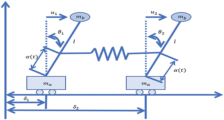
Figure 1. The inverted double pendulum system.

FIGURE 2

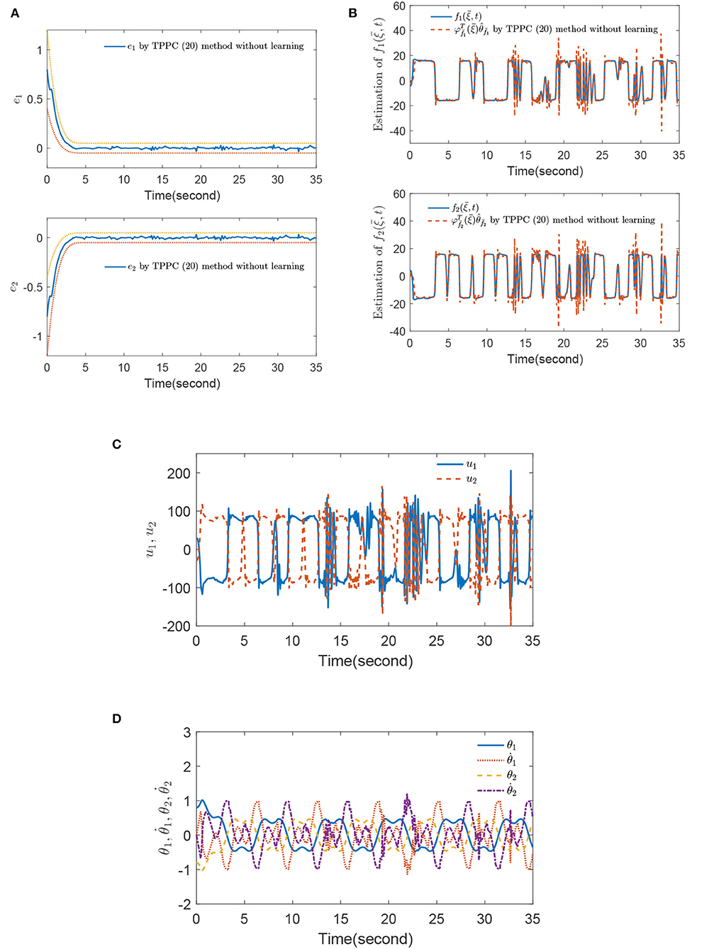
Figure 2. (A) Tracking errors e₁ and e₂, (B) estimation of $f_1(\stackrel{-}{\xi },t)$ and $f_2(\stackrel{-}{\xi },t)$, (C) control inputs u₁ and u₂, and (D) states ${\theta }_1,{\dot{\theta }}_1,{\theta }_2$, and ${\dot{\theta }}_2$ by using the time prescribed performance control (TPPC) method (Equation 20) without learning.

Figure 2A shows that tracking errors e₁ and e₂ are limited within PPBs (Equation 47). However, it was found that ${\phi }_{{\stackrel{-}{f}}_1}^T(\xi ){\widehat{\theta }}_{{\stackrel{-}{f}}_1}$ and ${\phi }_{{\stackrel{-}{f}}_2}^T(\xi ){\widehat{\theta }}_{{\stackrel{-}{f}}_2}$ appeared as some large jumps after 10 s in Figure 2B, indicating that the parameter updating law (Equation 21) cannot ensure that the unknown functions $f_1(\stackrel{-}{\xi },t)$ and $f_2(\stackrel{-}{\xi },t)$ are accurately estimated. From Figure 2C, one finds that each jump of controllers u₁ and u₂ is consistent with each fluctuation of ${\phi }_{{\stackrel{-}{f}}_1}^T(\xi ){\widehat{\theta }}_{{\stackrel{-}{f}}_1}$ and ${\phi }_{{\stackrel{-}{f}}_2}^T(\xi ){\widehat{\theta }}_{{\stackrel{-}{f}}_2}$, which indicates that the TPPC method (Equation 20) without learning cannot overcome the influence of dead-zone inputs Γ₁(ςu₁) and Γ₂(ςu₂). Meanwhile, Figure 2D shows that states ${\theta }_1,{\dot{\theta }}_1,{\theta }_2$, and ${\dot{\theta }}_2$ are recurrent, which also confirms the conclusion of Theorem 1.

Before using the method in Theorem 2, we need to verify whether $G(t)={\displaystyle {\int }_{t-{\tau }_d}^t}{\phi }_{\stackrel{-}{F}}^T(\stackrel{-}{\xi }){\phi }_{\stackrel{-}{F}}(\stackrel{-}{\xi })\text{d}\tau \ge \mu I$ is always true after time T_e + τ_d. According to Remark 2, we only need to verify that the minimum singular value of G(t) is greater than zero. The method in Theorem 2 was denoted as the TPPC (Equation 20) method with learning and let τ_d = 3 and

$\begin{array}{ll}{\lambda }_{min}=\{\begin{array}{rr}0,& t<T_d+{\tau }_d,\\ {\lambda }_{min}\left\{G(t)\right\},& t\ge T_d+{\tau }_d.\end{array}& (48)\end{array}$

Figure 3 shows that the selected fuzzy basic vector ${\phi }_{\stackrel{-}{F}}(\stackrel{-}{\xi })$ satisfies λ_min{G(t)} > 0 for t ≥ T_d + τ_d, which means that there is a constant μ such that G(t) ≥ μI holds. The simulation results of the IBPS by using the TPPC method (Equation 20) with learning are displayed in Figures 4A–C. By comparing Figure 2A with Figure 4A, the tracking error control effect of the TPPC method (Equation 20) with learning is obviously better than that of the TPPC method (Equation 20) without learning after T_e + τ_d. By comparing the estimation effect of unknown functions in Figures 2B, 4B, ${\phi }_{{\stackrel{-}{f}}_1}^T(\xi ){\widehat{\theta }}_{{\stackrel{-}{f}}_1}$ and ${\phi }_{{\stackrel{-}{f}}_2}^T(\xi ){\widehat{\theta }}_{{\stackrel{-}{f}}_2}$ do not show big fluctuation in Figure 4 by using the TPPC method (Equation 20) with learning and unknown functions $f_1(\stackrel{-}{\xi },t)$ and $f_2(\stackrel{-}{\xi },t)$ are estimated accurately. Figure 4C shows that controllers u₁ and u₂ were stable without large fluctuation by the TPPC method (Equation 20) with learning. Through the comparison of simulation results, the control effect of the TPPC method (Equation 20) with learning was obviously better than that of the TPPC method (Equation 20) without learning, which also confirmed the theoretical analysis of this paper.

FIGURE 3

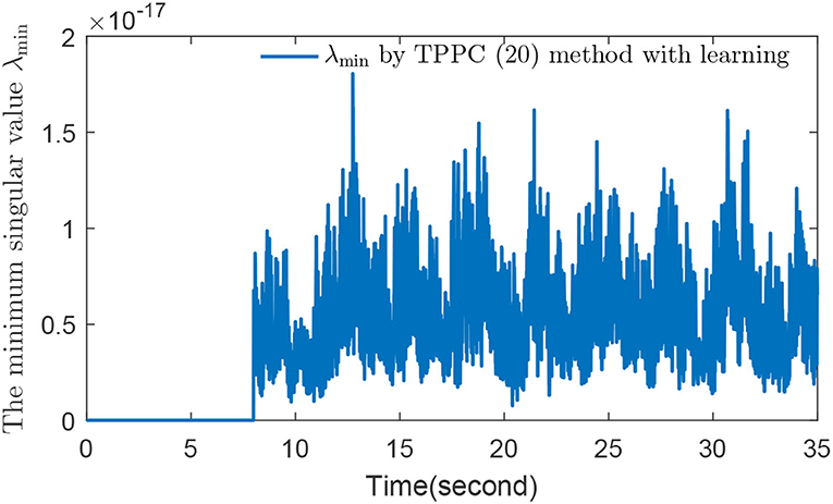
Figure 3. The minimum singular value λ_min of G(t).

FIGURE 4

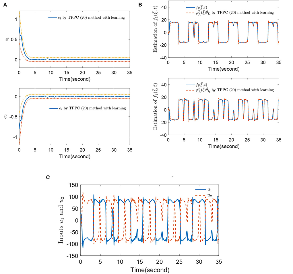
Figure 4. (A) Tracking errors e₁ and e₂, (B) estimation of $f_1(\stackrel{-}{\xi },t)$ and $f_2(\stackrel{-}{\xi },t)$, and (C) control inputs u₁ and u₂ by using the TPPC method (Equation 20) with learning.

5. Conclusion

In this paper, a composite learning finite-time PPC method was proposed for uncertain nonlinear systems with dead-zone inputs. A finite-time performance function and a transformation function were introduced, which can ensure that the racking error can be limited within a predefined region at a settling time. Then, in order to improve the accurate estimation effect of the unknown function, a prediction error was defined and a corresponding composite learning parameter law was designed. The simulation comparison of IBPS showed the superiority of the control effect of the proposed composite learning finite-time PPC method. Meanwhile, one can notice the limitation of the proposed method in this paper is that all states must be measurable. If some states are unmeasurable, the results of this paper cannot be obtained. Therefore, it is necessary to further study the problem of effective estimation of uncertainties based on partially measurable states.

Data availability statement

The original contributions presented in the study are included in the article/supplementary material, further inquiries can be directed to the corresponding author.

Author contributions

All authors listed have made a substantial, direct, and intellectual contribution to the work and approved it for publication.

Funding

This work was supported by the Natural Science Foundation for the Higher Education Institutions of Anhui Province of China (KJ2021A0965).

Conflict of interest

The authors declare that the research was conducted in the absence of any commercial or financial relationships that could be construed as a potential conflict of interest.

Publisher's note

All claims expressed in this article are solely those of the authors and do not necessarily represent those of their affiliated organizations, or those of the publisher, the editors and the reviewers. Any product that may be evaluated in this article, or claim that may be made by its manufacturer, is not guaranteed or endorsed by the publisher.

References

1. Lymperopoulos G, Ioannou P. Building temperature regulation in a multi-zone HVAC system using distributed adaptive control. Energy Build. (2020) 215:109825. doi: 10.1016/j.enbuild.2020.109825

CrossRef Full Text | Google Scholar

2. Wang P, Wen G, Huang T, Yu W, Lv Y. Asymptotical neuro-adaptive consensus of multi-agent systems with a high dimensional leader and directed switching topology. IEEE Trans Neural Netw Learn Syst. (2022) doi: 10.1109/TNNLS.2022.3156279 [Epub ahead of print].

PubMed Abstract | CrossRef Full Text | Google Scholar

3. El Hamidi K, Mjahed M, El Kari A, Ayad H. Adaptive control using neural networks and approximate models for nonlinear dynamic systems. Model Simul Eng. (2020) 2020:8642915. doi: 10.1155/2020/8642915

CrossRef Full Text | Google Scholar

4. Gammons MV, Renko M, Flack JE, Mieszczanek J, Bienz M. Feedback control of Wnt signaling based on ultrastable histidine cluster co-aggregation between Naked/NKD and Axin. Elife. (2020) 9:e59879. doi: 10.7554/eLife.59879

PubMed Abstract | CrossRef Full Text | Google Scholar

5. Nguyen AT, Coutinho P, Guerra TM, Palhares R, Pan J. Constrained output-feedback control for discrete-time fuzzy systems with local nonlinear models subject to state and input constraints. IEEE Trans Cybern. (2020) 51:4673–84. doi: 10.1109/TCYB.2020.3009128

PubMed Abstract | CrossRef Full Text | Google Scholar

6. Wang P, Yu W, Wen G, Yu X, Huang T. A chattering free consensus controller for multiple Lur systems with a non-autonomous leader and directed switching topology. Sci China Technol Sci. (2022). doi: 10.1007/s11431-022-2175-5

CrossRef Full Text

7. Wang P, Wen G, Huang T, Yu W, Ren Y. Observer-based consensus protocol for directed switching networks with a leader of nonzero inputs. IEEE Trans Cybern. (2020) 52: 630–40. doi: 10.1109/TCYB.2020.2981518

PubMed Abstract | CrossRef Full Text | Google Scholar

8. Wang S, Bekiros S, Yousefpour A, He S, Castillo O, Jahanshahi H. Synchronization of fractional time-delayed financial system using a novel type-2 fuzzy active control method. Chaos Solitons Fractals. (2020) 136:109768. doi: 10.1016/j.chaos.2020.109768

CrossRef Full Text | Google Scholar

9. Singh J, Jafari S, Khalaf A, Pham V, Roy B. A modified chaotic oscillator with megastability and variable boosting and its synchronisation using contraction theory-based control which is better than backstepping and nonlinear active control. Pramana. (2020) 94:1–14. doi: 10.1007/s12043-020-01993-y

CrossRef Full Text | Google Scholar

10. Li X, Peng D, Cao J. Lyapunov stability for impulsive systems via event-triggered impulsive control. IEEE Trans Automat Contr. (2020) 65:4908–3. doi: 10.1109/TAC.2020.2964558

CrossRef Full Text | Google Scholar

11. Stamov T, Stamova I. Design of impulsive controllers and impulsive control strategy for the Mittag-Leffler stability behavior of fractional gene regulatory networks. Neurocomputing. (2021) 424:54–62. doi: 10.1016/j.neucom.2020.10.112

CrossRef Full Text | Google Scholar

12. Bechlioulis CP, Rovithakis GA. Robust adaptive control of feedback linearizable MIMO nonlinear systems with prescribed performance. IEEE Trans Automat Contr. (2008) 53:2090–9. doi: 10.1109/TAC.2008.929402

CrossRef Full Text | Google Scholar

13. Niu B, Zhao J. Barrier Lyapunov functions for the output tracking control of constrained nonlinear switched systems. Syst Control Lett. (2013) 62:963–71. doi: 10.1016/j.sysconle.2013.07.003

CrossRef Full Text | Google Scholar

14. Li Y, Tong S. Prescribed performance adaptive fuzzy output-feedback dynamic surface control for nonlinear large-scale systems with time delays. Inf Sci. (2015) 292:125–42. doi: 10.1016/j.ins.2014.08.060

CrossRef Full Text | Google Scholar

15. Yao B, Tomizuka M. Smooth robust adaptive sliding mode control of manipulators with guaranteed transient performance. In: Proceedings of 1994 American Control Conference-ACC '94. Baltimore, MD: IEEE (1996).

Google Scholar

16. Zhi D, Xu L. Direct power control of DFIG with constant switching frequency and improved transient performance. IEEE Trans Energy Convers. (2007) 22:110–8. doi: 10.1109/TEC.2006.889549

CrossRef Full Text | Google Scholar

17. Kostarigka AK, Doulgeri Z, Rovithakis GA. Prescribed performance tracking for flexible joint robots with unknown dynamics and variable elasticity. Automatica. (2013) 49:1137–47. doi: 10.1016/j.automatica.2013.01.042

CrossRef Full Text | Google Scholar

18. Zhang L, Tong S, Li Y. Prescribed performance adaptive fuzzy output-feedback control of uncertain nonlinear systems with unmodeled dynamics. Nonlinear Dyn. (2014) 77:1653–65. doi: 10.1007/s11071-014-1407-0

CrossRef Full Text | Google Scholar

19. Zhang G, Cheng D. Observer-based neuro-adaptive prescribed performance control of nonstrict feedback systems and its application. Optik. (2019) 181:264–77. doi: 10.1016/j.ijleo.2018.12.018

CrossRef Full Text | Google Scholar

20. Bu X, Wu X, Huang J, Wei D. A guaranteed transient performance-based adaptive neural control scheme with low-complexity computation for flexible air-breathing hypersonic vehicles. Nonlinear Dyn. (2016) 84:2175–94. doi: 10.1007/s11071-016-2637-0

CrossRef Full Text | Google Scholar

21. Xiang W, Liu H. Fuzzy adaptive prescribed performance tracking control for uncertain nonlinear systems with unknown control gain signs. IEEE Access. (2019) 7:149867–77. doi: 10.1109/ACCESS.2019.2946601

CrossRef Full Text | Google Scholar

22. Liu Y, Liu X, Jing Y. Adaptive fuzzy finite-time stability of uncertain nonlinear systems based on prescribed performance. Fuzzy Sets Syst. (2019) 374:23–39. doi: 10.1016/j.fss.2018.12.015

PubMed Abstract | CrossRef Full Text | Google Scholar

23. Xiang W, Sun Y, Li N, Yang C. Uncertain chaotic gyros synchronization using adaptive fuzzy prescribed performance control with unknown dead-zone input. Int J Innovat Comput Inf Control. (2017) 13:429–440. doi: 10.1155/2017/4386515

CrossRef Full Text

24. Wang C, Hill DJ. Learning from neural control. IEEE Trans Neural Netw. (2006) 17:130–46. doi: 10.1109/TNN.2005.860843

PubMed Abstract | CrossRef Full Text | Google Scholar

25. Jamil ARM, Ganguly KK, Nower N. Adaptive traffic signal control system using composite reward architecture based deep reinforcement learning. IET Intell Transport Syst. (2021) 14:2030–41. doi: 10.1049/iet-its.2020.0443

CrossRef Full Text | Google Scholar

26. Pan Y, Zhou Y, Sun T, Er MJ. Composite adaptive fuzzy H_∞ tracking control of uncertain nonlinear systems. Neurocomputing. (2013) 99:15–24. doi: 10.1016/j.neucom.2012.05.011

CrossRef Full Text | Google Scholar

27. Pan Y, Yu H. Composite learning from adaptive dynamic surface control. IEEE Trans Automat Contr. (2015) 61:2603–9. doi: 10.1109/TAC.2015.2495232

PubMed Abstract | CrossRef Full Text | Google Scholar

28. Soukkou Y, Labiod S, Tadjine M. Composite adaptive dynamic surface control of nonlinear systems in parametric strict-feedback form. Trans Inst Meas Control. (2018) 40:1127–35. doi: 10.1177/0142331216675672

CrossRef Full Text | Google Scholar

29. Liu H, Pan Y, Cao J. Composite learning adaptive dynamic surface control of fractional-order nonlinear systems. IEEE Trans Cybern. (2019) 50:2557–67. doi: 10.1109/TCYB.2019.2938754

PubMed Abstract | CrossRef Full Text | Google Scholar

30. Liu H, Pan Y, Li S, Chen Y. Adaptive fuzzy backstepping control of fractional-order nonlinear systems. IEEE Trans Syst Man Cybern Syst. (2017) 47:2209–17. doi: 10.1109/TSMC.2016.2640950

PubMed Abstract | CrossRef Full Text | Google Scholar

31. Pan Y, Sun T, Yu H. Composite adaptive dynamic surface control using online recorded data. Int J Robust Nonlinear Control. (2016) 26:3921–36. doi: 10.1002/rnc.3541

PubMed Abstract | CrossRef Full Text | Google Scholar

32. Pan Y, Yu H. Composite learning robot control with guaranteed parameter convergence. Automatica. (2018) 89:398–406. doi: 10.1016/j.automatica.2017.11.032

CrossRef Full Text | Google Scholar

33. Wang M, Yang A. Dynamic learning from adaptive neural control of robot manipulators with prescribed performance. IEEE Trans Syst Man Cybern Syst. (2017) 47:2244–55. doi: 10.1109/TSMC.2016.2645942

CrossRef Full Text | Google Scholar

34. Hu J, Zhang H. Immersion and invariance based command-filtered adaptive backstepping control of VTOL vehicles. Automatica. (2013) 49:2160–7. doi: 10.1016/j.automatica.2013.03.019

CrossRef Full Text | Google Scholar

35. Lin CM, Chung CC. Fuzzy brain emotional learning control system design for nonlinear systems. Int J Fuzzy Syst. (2015) 17:117–28. doi: 10.1007/s40815-015-0020-9

PubMed Abstract | CrossRef Full Text | Google Scholar