Herbicide resistance prediction: a mechanistic model vs. a random forest model

Introduction: Herbicides are an important technology in the Integrated Weed Management (IWM) tool box aiming to control weeds in modern agriculture. Prediction tools to evaluate the risk of resistance evolution will greatly help to choose the best IWM strategy adapted to the local field situation. These comprise classical simulation models, mechanistic models (MMs), combining population dynamics and genetics, and recently artificial intelligence (AI) methods such as random forest. In this paper, both approaches are compared.

Materials and methods: Artificial data were generated by an MM and used as training dataset for a random forest classifier. Field history information was taken from two previous studies. The data include the field histories and resistance status of Alopecurus myosuroides of 98 fields from the Hohenlohe area in Germany and 131 from the Champagne area in France.

Results and discussion: With accuracies of approximately 80%, the results obtained by the random forest method applied to model-generated data and real field data, respectively, are well comparable. This concerns the ranking of prediction variables and the prediction of the resistance status of a real field and a “model field”. Predictions with model outcomes as training sets and, vice versa, predictions of a “model field” with real data as training sets and predictions by splitting of field data could be made with nearly the same accuracies.

Conclusion: Complementarity is shown between both approaches with the advantages of AI such as random forest to avoid approximations inherent to complex MMs.

Introduction

In the last decades, herbicide resistance in weeds has become a major issue (Gressel, 2009, Powles and Yu, 2010). Control of weed populations is a complex process depending not only on the choice of appropriate herbicides but also on cropping patterns, cultural techniques, and other crop management practices (Hawkins et al., 2019). The time scales involved in resistance evolution comprise several years. Weed population dynamics is a multifactorial process. Variables such as weather conditions, size and spatial heterogeneity of the seedbank, initial frequency of resistant biotypes, and spray distribution patterns exhibit a large variation (Zwerger et al., 2017). Therefore, the evolution of resistance is not a pure deterministic process.

One way to assess appropriate management schemes is based on mathematical process models (Colbach and Debaeke, 1998; Holst et al., 2007; Renton et al., 2014). The advantages of mechanistic models (MMs) are that they are based explicitly on population dynamics and genetics and are capable of analyzing underlying mechanisms. The disadvantage is that these models demand a large input of physiological parameters such as emergence rate, number of seeds, seed survival, vertical transport parameters due to soil cultivation, competition coefficients with respect to crops, and environmental variables. The second approach to evaluate the factors for the emergence of resistance is based on statistical methods notably on techniques of artificial intelligence (AI). The advantage of these methods is that they are capable of detecting patterns in huge bodies of data, allowing the identification of the driving forces for resistance evolution. In addition, this approach is based on empirical parameters, usually easy to measure, like crop rotation, soil management, agronomic practices, and herbicide management including application rates. Disadvantages are that large data comprehending long-term field histories are needed requiring the compliance of the farmers partaking in the study. Furthermore, outcomes are frequently difficult to interpret in terms of the underlying mechanisms. The automatic learning methods (AI) are evolving fast and are implemented in a wide range of fields. The traditional MMs, depending on complex interdependent mechanisms (e.g., biological and genetic), are evolving towards statistical models (AI) evaluated on their single ability of prediction (Gabrié and Eickenberg, 2024). Our study focuses on the grass weed Alopecurus myosuroides Huds. (ALOMY). This grass mostly occurs in Central and Western Europe, where it has established itself as a noxious weed. Furthermore, owing to the evolution of resistance to acetyl-CoA carboxylase (ACCase), acetolactate synthase (ALS), and photosynthesis (PSII) inhibitors, this weed has become one of the most problematic weed species in Europe (Moss et al., 2007; Menne and Hogrefe, 2012). Herrmann (2016) examined the evolution of resistance to ALS and ACCase inhibitors and compared MM results and the results obtained by a random forest (RF) classifier (AI) applied to field history data of the Hohenlohe region in Germany. In this paper, field data were taken from the field history data from Hohenlohe and from Champagne in France (Lepke et al., 2024). In addition, for this study, data were generated by an MM with the objective to compare mechanistic modeling and AI separately and in combination. To this end, model-derived data were used as training dataset for an RF classifier. A time discrete model was developed, which combines the population dynamics and genetics of this grass independent of management schemes comprising application of herbicides with different modes of action in spring and autumn, selection of crops, seeding dates, and soil cultivation. The algorithm produces time courses of the seedbank bank and weed densities for each biotype and determines the resistance status of a field at the end of the simulation period. The model contains stochastic features concerning the emergence of the weed, the efficacy of herbicide treatment, and the detection of resistance by random sampling of weeds. The questions addressed are as follows: (1) is it feasible to obtain reliable predictions on resistance evolution using a model generated database as training set? and (2) which training database, field data or model data, yields the best predictions?

Materials and methods

Field history data

Field history data were taken from two previous studies. The data include the field histories and resistance status of black-grass of 98 fields from the Hohenlohe area in Germany (Herrmann, 2016; Lepke et al., 2020) and of 131 fields from the Champagne area in France (Lepke et al., 2024). Predictor variables comprise crop rotation, number of crops, seeding date, soil cultivation, and herbicide applications. There are 20 predictors (Table 1). The Hohenlohe data include soil properties, which were not recorded in the French study. An additional predictor management diversity was devised, which is an index for the diversity of A. myosuroides management (Herrmann, 2016). This variable considers the number of different measures specific for weed control within a year. These comprise delayed seeding, ploughing, summer crops, and the use of multiple modes of action. If a measure is applied, the respective score takes the value of 1; otherwise, the value of 0. If all measures are applied, the maximum value of management diversity is 4; if none is applied, the score is 0. The index ranges therefore between 0 and 4. For example, in winter wheat, using two modes of action (score 1) and ploughing (score 1) results in a management diversity value of 2, while shallow tillage (score 0) and only one mode of action (score 0) give a management diversity value of 0. Management diversity values are averaged for the time frame of the 6 years (6 yrs) being considered.

Table 1

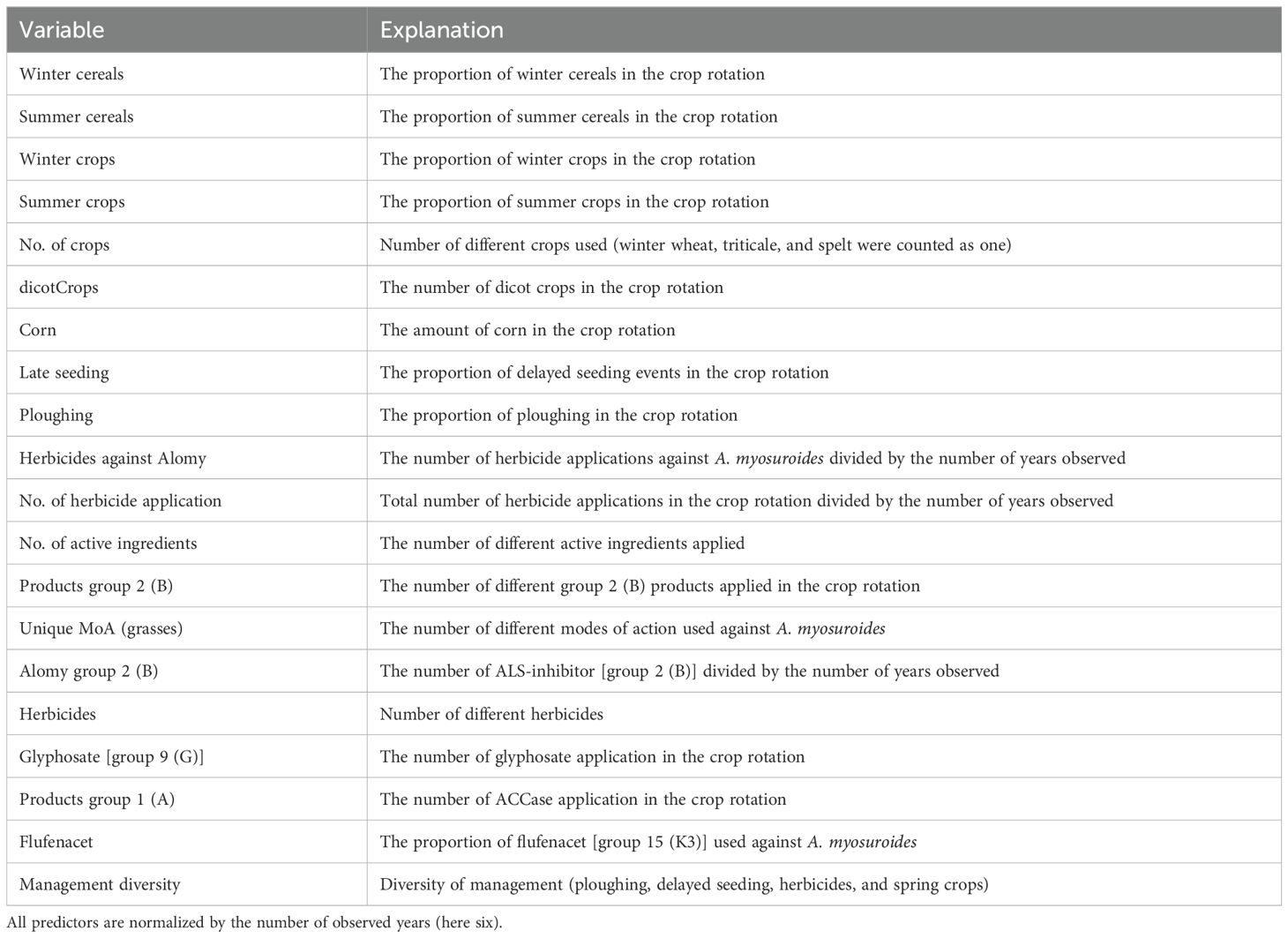
Table 1. List of predictor variables (Lepke et al., 2024).

A descriptive data analysis was performed to ensure that the datasets of both countries have a similar structure (Lepke et al., 2020, 2024). There are only slightly different management practices concerning late seedings and summer crops. In France, herbicides that are specific for A. myosuroides are applied more frequently than in Germany. In both regions, non-inversion tillage is common. The correlation structures of the predictor variables are similar for both datasets of A. myosuroides (Lepke et al., 2020). Climatic conditions are slightly different in the two regions; mean temperature and precipitation are slightly higher in the Champagne than in the Hohenlohe region.

Assessment of resistance status

The field data used in this paper were obtained from previous studies (Herrmann et al., 2016; Lepke et al., 2024). A. myosuroides samples were harvested by walking every second tractor track and monitoring two borders of the field. It was ensured that only one ear per plant was sampled. Resistance status was established by greenhouse biotests with collected seeds and subsequent genetic analysis of the seedlings to determine target site resistance and analytics to determine metabolic resistance when appropriate for the samples from Champagne and Hohenlohe (Lepke et al., 2020, 2024; Beffa et al., 2012). Fields were classified as resistant if target-site resistance or metabolic resistance or both were detected in the samples and/or survivals were observed in the greenhouse. More than 95% of the samples showed the presence of target site resistance. Therefore, the model was focused on target site resistance risk evolution. The stochastic process of the assessment of the resistance status is part of the model.

Simulation model

Basic population dynamics

Notations:

The term “biotype” used in weed resistance (and in the paper) is synonymous to the term “phenotype” in genetic literature. One biotype represents the population of one field.

S_i: number of seeds of biotype i.

P_A: emergence rate.

K_i: number of seedlings of biotype i.

J_i: number of young plants of biotype i.

D_max: maximum density of seedlings.

L: half maximum seedling density.

h: herbicide dose.

Su_i(h): survival probability of biotype i under herbicide dose h.

R=(R₁,…,R_n): vector of adult plants.

A_max: maximum number of seeds per plant.

a,b: competition coefficients with respect to weeds and crop.

g_i (R): offspring rate of biotype i (cf. also Equation 11).

p_s,p_w: seed survival in summer and winter, respectively.

The model simulates the population dynamics and genetics of A. myosuroides with target site resistance against ALS inhibitors. The model structure and the parameterization were taken from Herrmann (2016). It is assumed that resistance is conferred by one locus. The model is capable of taking into account multiple target site resistance. In this study, only target site resistance against ALS inhibitors was considered in accordance with our field data (Lepke et al., 2020, 2024).

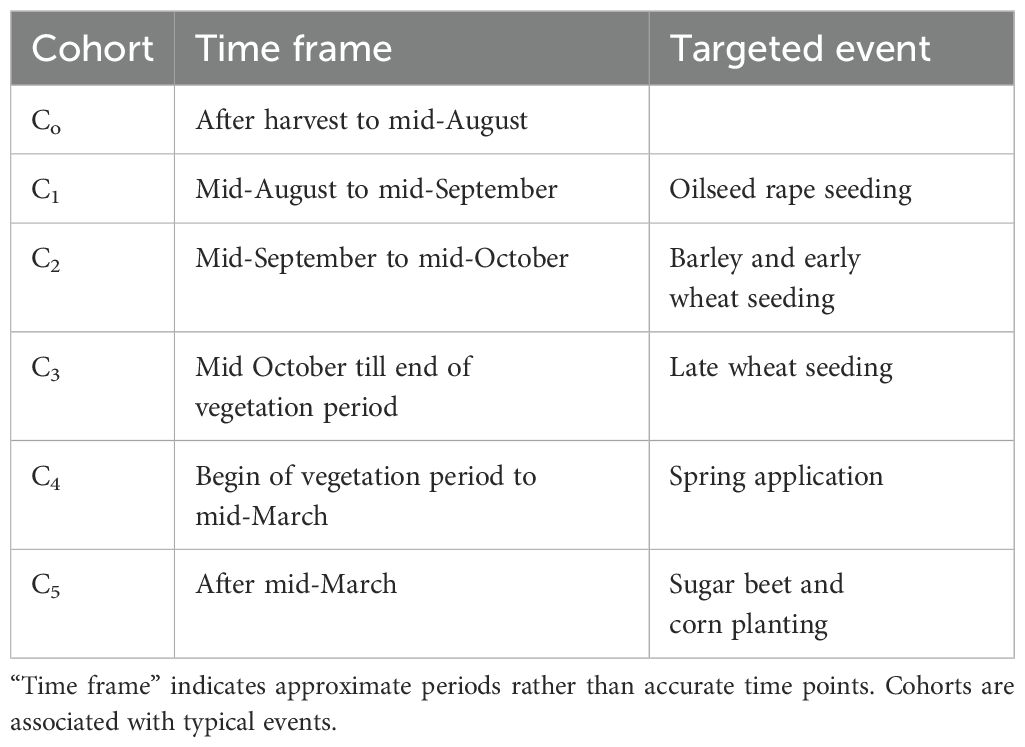
The weed population is composed of six cohorts representing different seasonal phases (Table 2). The structure of the model is shown in Figure 1. In each cohort, the population dynamics and genetics evolve according to a time discrete model comprising the stages seedling, juvenile plant, and adult plant. At the beginning of a cycle, K seedlings germinate from the seed bank (Equation 2). The index “i” denotes the biotype.

Table 2

Table 2. Germination cohorts of A. myosuroides.

Figure 1

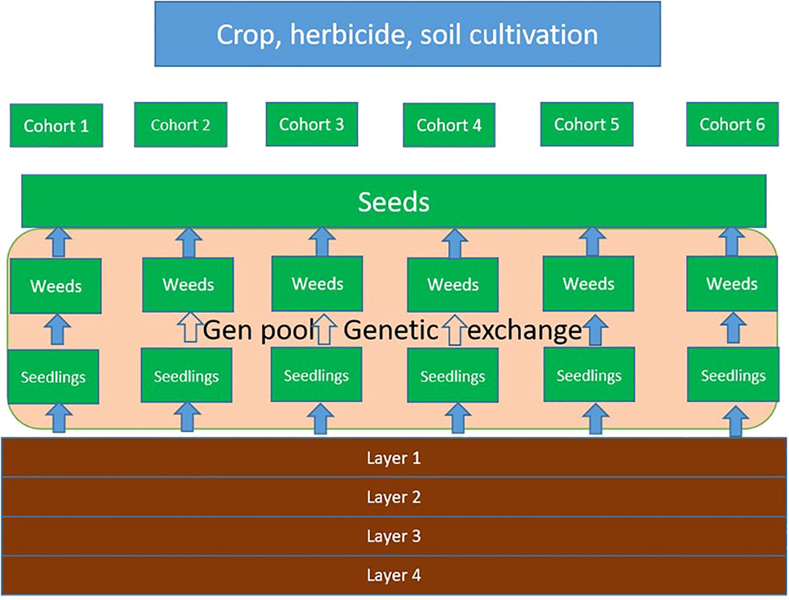
Figure 1. Model structure. The cohorts represent different seasonal phases that are associated with typical events such as herbicide application or seeding.

$\begin{array}{ll}{K}_i=p_A{S}_i& (1)\end{array}$

The survival of the seedlings is density dependent. The number of seedlings that develop to juvenile plants is limited by D_max.

$\begin{array}{ll}{J}_i=\frac{D_{\max }K}{K+L}\frac{K_i}{K}& (2)\end{array}$

The development to mature plants depends on the survival probability Su_i under herbicide dose h, which is given by a dose–response function with biotype-specific parameters.

$\begin{array}{ll}{R}_i=J_{i}S{u}_i(h)& (3)\end{array}$

The portion of seeds with biotype i is derived via the hereditary transmission matrix W_i (Equation 10) as.

$\begin{array}{ll}{g}_i(R)=\frac{R^t{W}_{i}R}{R_{total}^2}& (4)\end{array}$

The number of seeds per weed plant depends on crop and weed densities.

$\begin{array}{ll}{S}_{Hi}=\frac{A_{max}}{{(1+a{R}_{total}+b{D}_{Crop})}^{\gamma }}{g}_i(R)& (5)\end{array}$

At the beginning of the next cycle, the seed bank adds up to.

$\begin{array}{ll}{S}_{F(t+1)}{i}_{=}(S_{Ft}i(1-p_A)p_s+S_{Hi})p_w& (6)\end{array}$

where p_s and p_w denote the seed survival probability over summer and winter, respectively.

$$K={\displaystyle {\sum }_{i=1}^m{K}_i}$$

$$R={(R_1,\cdots ,R_m)}^t$$

$$R_{total}={\displaystyle {\sum }_{i=1}^{nbio}{R}_i}$$

Multiple resistance

Under the assumption that multiple resistance is conferred independently by one locus for each herbicide, rates of offspring are derived by tensor products of heredity matrices [7,8,9]. Biotypes Ri are ordered lexicographically with respect to the alleles X_j and x_j occurring in the gene. Elementary heredity transmission matrices for single genes can be represented by.

$\begin{array}{ll}{V}_1=\left(\begin{array}{ccc}1& 1/2& 0\\ 1/2& 1/4& 0\\ 0& 0& 0\end{array}\right)& (7)\end{array}$

$\begin{array}{ll}{V}_2=\left(\begin{array}{ccc}0& 1/2& 1\\ 1/2& 1/2& 1/2\\ 1& 1/2& 0\end{array}\right)& (8)\end{array}$

$\begin{array}{ll}{V}_3=\left(\begin{array}{ccc}0& 0& 0\\ 0& 1/4& 1/2\\ 0& 1/2& 1\end{array}\right)& (9)\end{array}$

and they can be written as the tensor products in the multi-loci case transmission matrices W_i are obtained from the Kronecker product of the single transmission matrices.

$\begin{array}{ll}{W}_i=V_{i1}\otimes V_{i2}\otimes \cdots \otimes V_{im}& (10)\end{array}$

with the number m of gene loci and with biotypes ordered again lexicographically with respect to multiple gene loci. The fraction of biotype i in the population after random mating is termed normed heredity function and is derived via the hereditary matrices as

$\begin{array}{ll}{g}_i(R)=\frac{R^t{W}_{i}R}{R_{total}^2}& (11)\end{array}$

Equation 11 gives the rates of offspring of each biotype, and thus, it is the basis for dynamic population genetic models.

Seedbank

The soil is divided into four layers (0–5 cm, 5–10 cm, 10–15 cm, and 15–20 cm). Seed emergence takes place from the upper layer. For the mixing of the layers by soil cultivation, the model of Cousens and Moss (1990) was taken. The mixing of soil layers is accomplished via matrix operators applied to soil layer vectors. For each soil cultivation technique ploughing, rigid tine cultivation and minimal cultivation-specific matrix elements apply. P is the soil cultivation matrix for four soil layers. For each soil cultivation technique ploughing, rigid tine cultivation and minimal cultivation-specific matrix elements apply.

Stochastic features

In the model seed emergence, number of seeds per plant, herbicide efficacy, and the initial fractions of resistant seeds in the seedbank are considered as random. For each of the respective parameters, a plausible range was chosen. In a simulation run, the value of the parameter was determined by a uniformly distributed random variable.

The assessment of the resistance status is a two-stage stochastic process. In the first step, n_f plants are randomly sampled. In the second step, mixed seedling samples from these plants are grown and n_lab samples are taken. A field is classified as resistant if at least 2 weed plants out of 8 grown from seeds of 10 plant samples from the field are resistant. The effect of sampling on resistance detection was studied in Herrmann et al. (2022).

Management schemes

The management schemes comprise the selection of herbicides out of seven herbicides with different modes of action, application rate, application period (spring or autumn), soil cultivation such as ploughing, cultivation with tine and direct seed, and the growing of 11 crops (Herrmann et al., 2022).

Random forest

For a classification problem with 20 predictor variables, partly correlated samples, and small sample sizes, the RF method (Breiman, 2001) is the most convenient. All calculations were carried out by the R Project for Statistical Computing (R Core Team, 2018; R-package‚ ‘random forest’, 2018). In all analyses, the data were split into training data (75%) and test data (25%). To test which predictor variables have a significant impact on the response, importance measures were analyzed. Usual importance measures are the Gini index, the mean decrease accuracy index, and the area under the receiver operating characteristic curve (AUC) (Hastie et al., 2017). RF outcomes are random due to random sampling of training data points when building trees and the random selection of subsets of features considered when splitting nodes. Therefore, the evaluation of feature importance based on a single run is not reliable especially if predictor variables are correlated. To assess the importance of prediction variables, RF analyses were performed for each dataset separately with the usual random splitting of training and test data with a ratio of 75% and 25%, respectively. Statistics of performance measures were generated by 50 simulation runs respectively.

Results and discussion

Model performance

Figure 2 shows the graphical user interface of the model. The user may select among seven herbicides or group of herbicides, application rates, and application period among 14 crops and soil cultivation for each year. In addition, parameters for the random feature of such random seeds and variation coefficients can be chosen. The model output comprises time series of the portion of resistant seeds, weed density, and others (see Figure 3). Figure 3B presents the results of a sampling for resistance (0: no resistance detected, 1: resistance confirmed). The figure shows what can happen in the worst case, when always the same herbicide (here ALS inhibitor) and the same crop are chosen. Until year 6 to 7, the seedbank is decreasing. From year 7 onward, a sharp rise in resistant weeds occurs. Resistance is confirmed only in year 9. Under a management scheme with a high degree of diversity, i.e., frequent change of mode of action and crop rotation (Figure 4), resistance development is delayed during the simulation period.

Figure 2

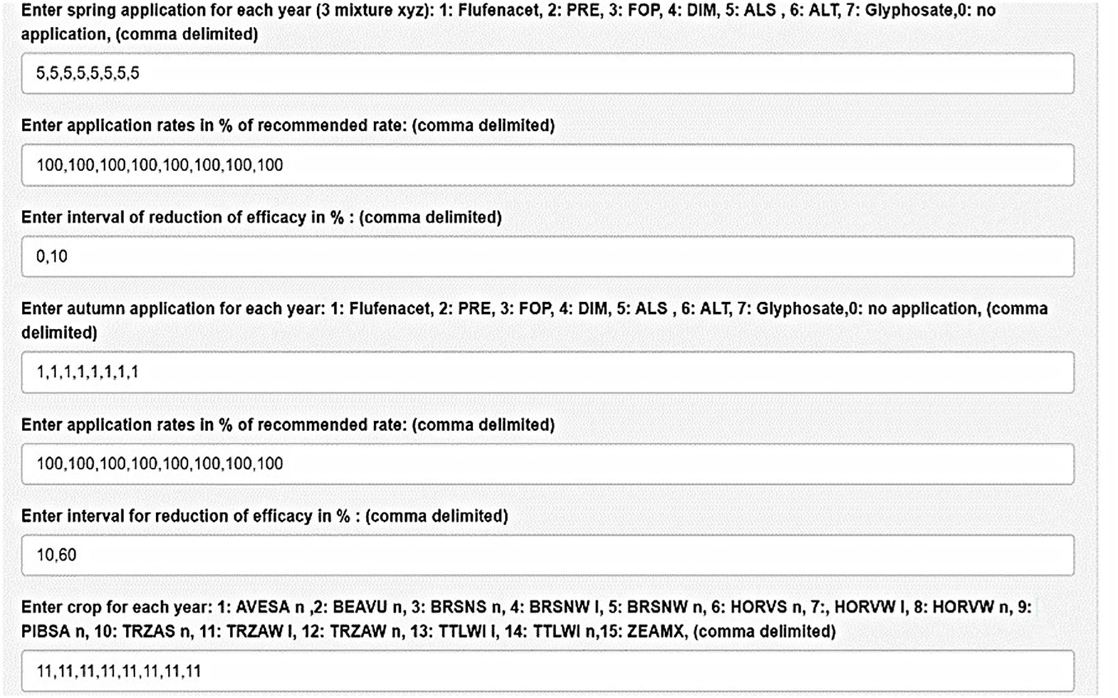
Figure 2. Graphical user interface. The simple management scheme of this example [always ALS inhibitor, always the same crop (Triticum aestivum winter)] favors fast emergence of resistance as shown in the next figure.

Figure 3

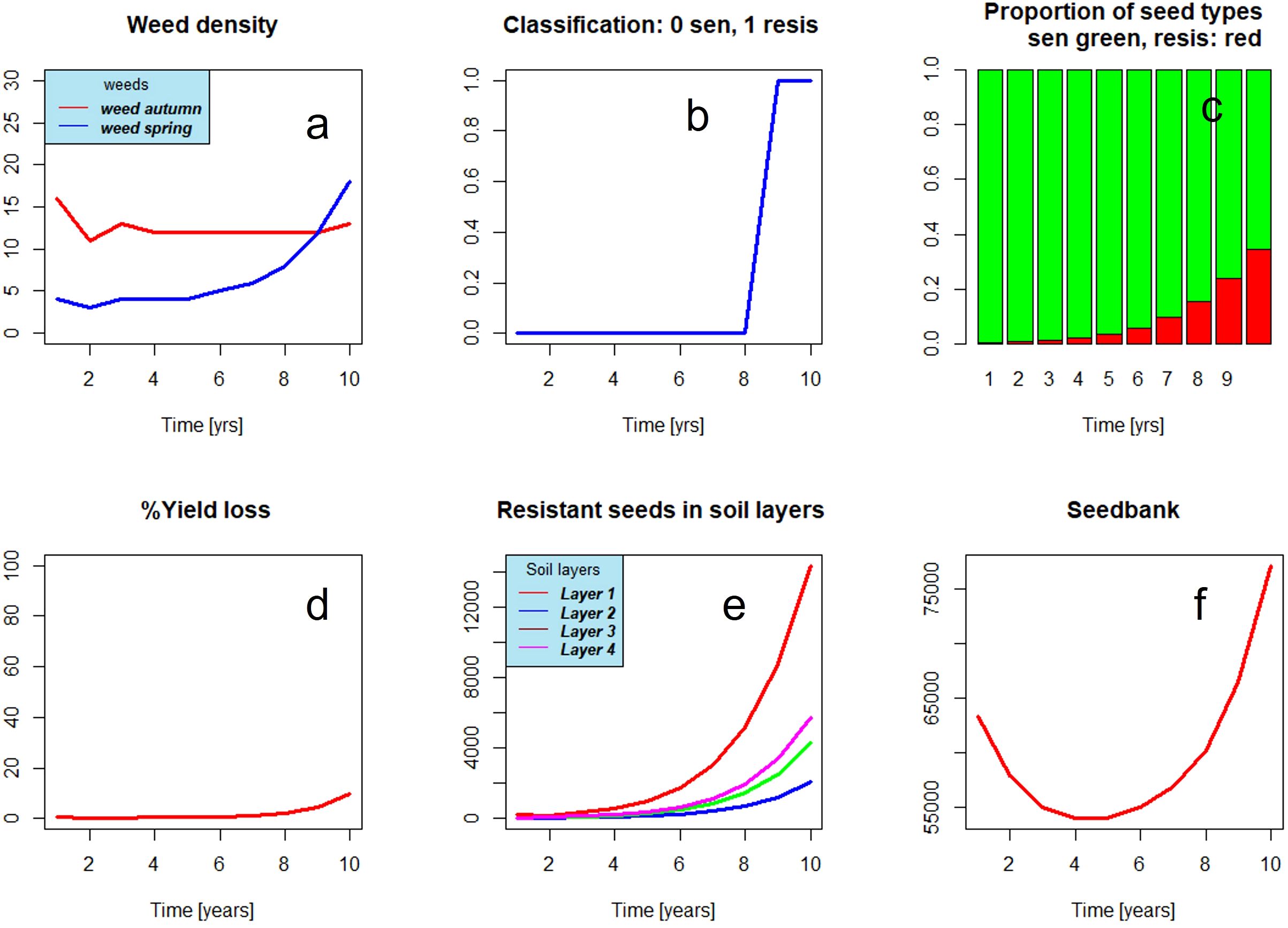
Figure 3. Weed dynamics under subsequent applications of an ALS inhibitor, no crop rotation, no change of mode of action. Resistance emerges after 4 to 5 years (C) and is detected only in year 9 (B). Because of ploughing, resistant seeds emerge in all soil layers (E). Weed densities are increasing after 8 years (A) causing crop losses (D). The seedbank, which is decreasing in the beginning, increases after 6 to 7 years (F).

Figure 4

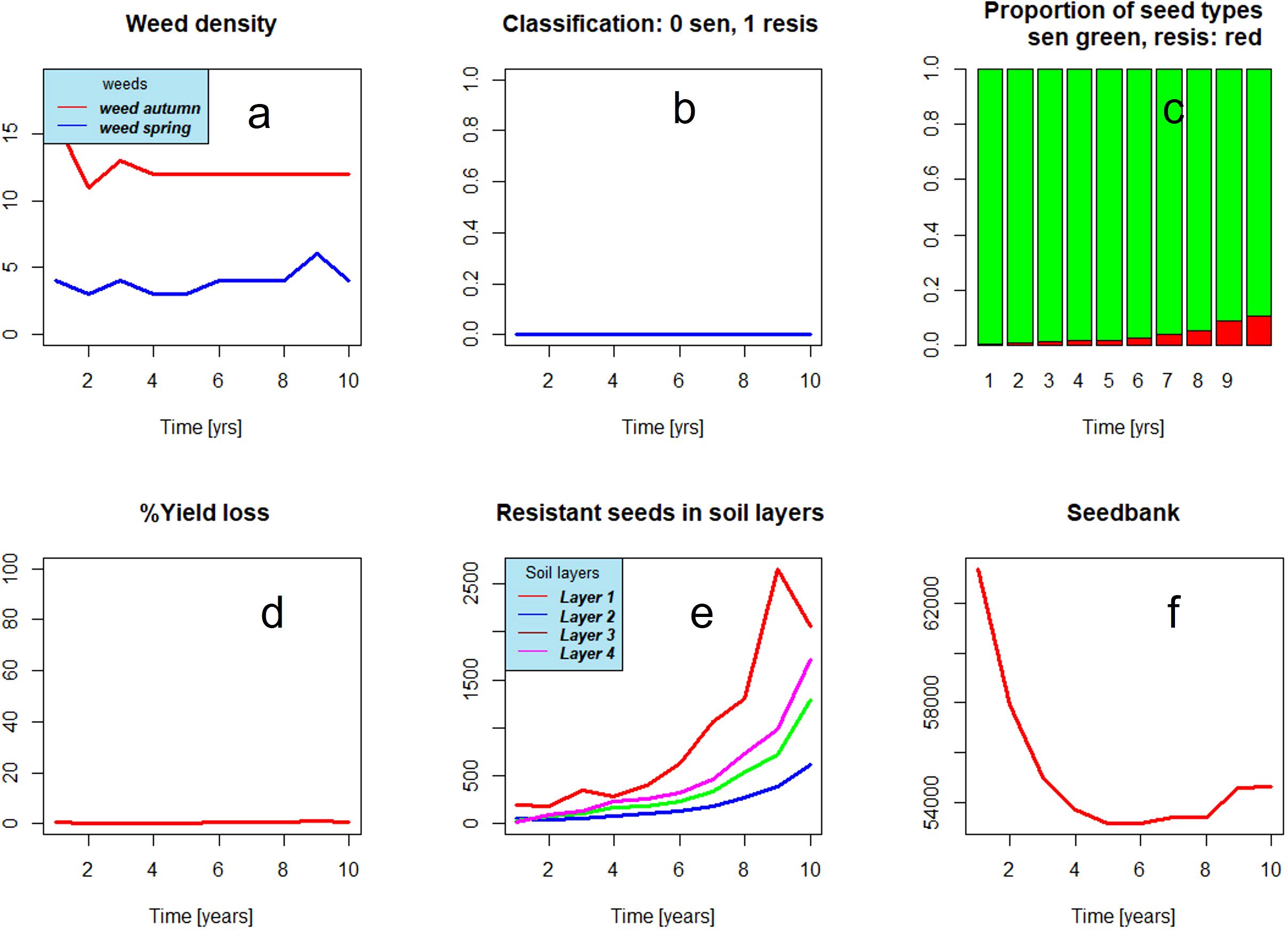
Figure 4. Weed dynamics under a management scheme comprising frequent changes of modes of action and crop rotation corresponding to a high value of variable management diversity, which is an index for the diversity of management. The development of resistance is delayed (C). Resistance is not detected (B). The seedbank decreases and stabilizes at low values (F). Weed densities stay at a low level (A) and no crop losses occur (D).

Predictions of resistance of field data based on model data

The field data are taken from previous studies (Lepke et al., 2024). The MM data were obtained from the model described above. These were generated in accordance with the field history data over a period of 6 years. In addition, simulations were performed with time horizons greater than 6 years, showing that under some management schemes, resistance in development was too low to be detected after 6 years but only later. Therefore, some datasets were generated with a simulation time of 8 years. Because of the random features in the model, identical management scenarios were repeated several times. Resistance status was determined by taking a random sample of five weed plants at the end of the simulation period and the field was classified as resistant if at least one of the plants was found to be resistant. Further datasets were generated with the pure deterministic model and on the model with all stochastic features described above. As usual, model data were split into a training sample (75%) and into a prediction sample (25%). It turned out that the model dataset obtained for an 8-year simulation period with stochastic features gave the best results. Further analyses were therefore performed with this dataset.

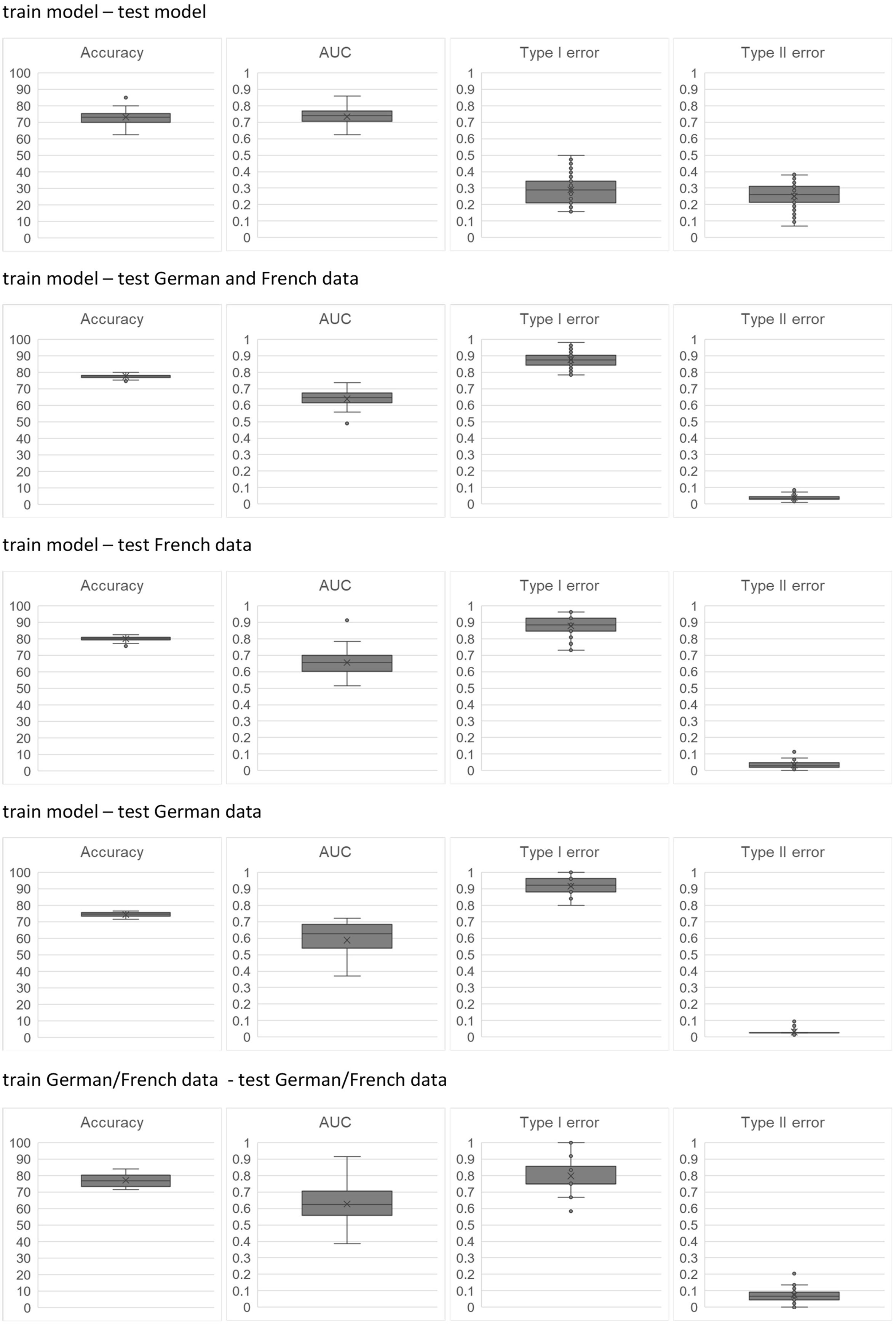
The final question remains: which predictions are better, those based on real datasets only or those based on model data. This question is answered in Figure 5 where performance criteria are compared for five combinations of training and test data: test data model generated (1); training data model generated (2); training data model generated and test data GER and FRA combined (3); training data model, test data FRA, training data model, and test data GER (4); and finally test and training data combined GER and FRA data (5).

Figure 5

Figure 5. Performance criteria for five combinations of training and test data.

With the exception of combination (1), mean accuracies range between 75% and 80%. It is interesting to note that all predictions based on model data have lower variations than predictions based on real data. AUC values exhibit large variation for all combinations. In those combinations with real data as test sets, type II errors are lower than type I errors, i.e., false-positive classifications are more frequent. There are two possible explanations:

The misclassified sensitive field has features similar to the features of resistant fields, but resistance has not developed as yet or has not been found in the plant samples.

There are other factors not considered, e.g., soil properties and weather patterns.

Variable importance

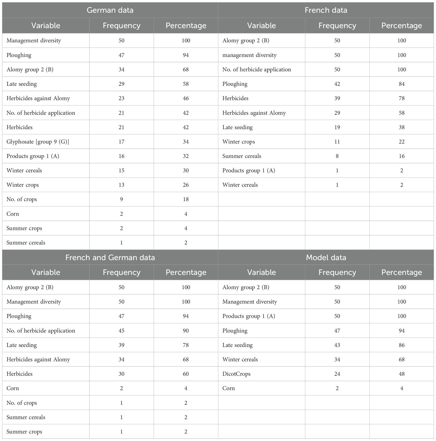
Statistics of performance measures were generated by 50 simulation runs respectively (cf. methods). Table 3 shows the frequencies of prediction variables falling into the group of the nine highest-ranked importance measures in 50 RF runs with randomly split training and test datasets for the two cases considered. It turns out that the prediction variables Alomy group 2 (B), the index management diversity, ploughing, and the proportion of late seeding are among the most frequent common ranks for combinations of training and datasets.

Table 3

Table 3. Importance of prediction variables for each dataset.

Discussion and conclusions

This paper is a synthesis of previous studies and combines field surveys, data analysis, and modeling. In a first study (Herrmann et al., 2016), an RF procedure was trained with data from Germany (Hohenlohe). Later, data from France (Champagne) were added to investigate transferability (Lepke et al., 2024). In parallel, a detailed MM to predict the emergence of resistance was developed (Herrmann et al., 2022). Our study presents the latest version of this model. The model is able to predict resistance for different management systems such as tillage and herbicide application schemes. This makes it possible to compare datasets from France and Germany and datasets generated by the model in different combinations in terms of variable importance. Since the RF procedure is a two-stage random procedure, the ranking of the predictor variables cannot be based on a single analysis but must be based on statistics from a large number of runs. The most important result is that the predictor variables Alomy group 2 (B), the index management diversity, ploughing, and the proportion of late-seeding are among the most frequent common ranks for combinations of training and datasets.

We have shown that the results of the RF method applied to model generated data (MM data) and real field data respectively are well comparable. This concerns the ranking of prediction variables and the prediction of the resistance status of a real field and a “model field”. Predictions with model outcomes as training sets and, vice versa, predictions of a “model field” with real data as training sets, and predictions by splitting of field data could be made with nearly the same accuracies.

This motivates a reflection of what is an MM in contrast to an AI algorithm. First, there exists no general rule let alone an algorithm for the development of a mathematical model. A model is based on expert knowledge derived from a variety of sources—own experience, exchange with other experts, literature, and population dynamics—and genetic theory and not least on intuition. The formal structure of a mathematical model allows its adaptation to other herbicides and crops. In contrast, an AI algorithm is capable of identifying structures in large bodies of data and making good predictions without “being aware” of the underlying mechanisms. A further advantage of this method is that the performance of the algorithm is improving with increasing number of cases. Our studies have shown that both approaches are in a way complementary to each other. AI offers the possibility to generate a correct prediction and avoid to generate very complex equations and calculations. Furthermore, each time that new data are generated, the algorithm is improving. However, one basic problem of AI models is that it is very difficult to anticipate errors generated by the model itself (Gabrié and Eickenberg, 2024). Therefore, it is reassuring that human intuition and calculations (MMs) and AI give the same results when it comes to the prediction of resistance evolution. Such prediction allows the customers, particularly the farmers, to evaluate the risks of resistance evolution and, taking into account the local conditions, proactively adapt the strategy of weed control to mitigate resistance evolution. It also allows farmers to not depend on complex diagnostics, especially related to non-target-site resistance (Lowe et al., 2024). This will contribute to develop the best Integrated Weed Management strategies combining chemical and agronomical measures.

Data availability statement

The raw data supporting the conclusions of this article will be made available by the authors, without undue reservation.

Author contributions

OR: Methodology, Project administration, Writing – original draft. JL: Investigation, Software, Writing – review & editing. JH: Data curation, Investigation, Writing – review & editing. RB: Conceptualization, Validation, Writing – review & editing.

Funding

The author(s) declare financial support was received for the research, authorship, and/or publication of this article. This research was funded partly by Bayer CropScience.

Conflict of interest

Author JH was employed by the company Agris42 GmbH.

The remaining authors declare that the research was conducted in the absence of any commercial or financial relationships that could be construed as a potential conflict of interest.

Publisher’s note

All claims expressed in this article are solely those of the authors and do not necessarily represent those of their affiliated organizations, or those of the publisher, the editors and the reviewers. Any product that may be evaluated in this article, or claim that may be made by its manufacturer, is not guaranteed or endorsed by the publisher.

References

Beffa R., Figge A., Lorentz L., Hess M., Laber B., Ruiz-Santaella J. P., et al. (2012). Weed resistance diagnostic technologies to detect herbicide resistance in cereal growing areas. A review. Julius-Kühn-Archiv 434, 75–80. doi: 10.5073/jka.2012.434.008

Crossref Full Text | Google Scholar

Breiman L. (2001). Random forest. Mach. Learn. 45, 5–32. doi: 10.1023/A:1010933404324

Crossref Full Text | Google Scholar

Colbach N., Debaeke P. (1998). Integrating crop management and crop rotation effects into models of weed populationdynamics: a review. Weed. Sci. 46, 717–728. doi: 10.1017/S0043174500089761

Crossref Full Text | Google Scholar

Cousens R., Moss S. R. (1990). A model of the effects of cultivation on the vertical distribution of weed seeds within the soil. Weed. Res. 30, 61–70. doi: 10.1111/j.1365-3180.1990.tb01688.x

Crossref Full Text | Google Scholar

Gabrié M., Eickenberg M. (2024). Un nouvel outil pour le calcul scientifique. La. Recheche. 577, 46–50.

Google Scholar

Gressel J. (2009). Evolving understanding of evolution of herbicide resistance. Pest Manage. Sci. 65, 1164–1173. doi: 10.1002/ps.v65:11

PubMed Abstract | Crossref Full Text | Google Scholar

Hastie T., Tibshirani R., Friedman J. (2017). The Elements of Statistical Learning. 2nd ed (New York: Springer Verlag), 593 p.

Google Scholar

Hawkins N. J., Bass C., Dixon A., Neve P. (2019). The evolutionary origins of pesticide resistance. Biol. Rev. 94, 135–155. doi: 10.1111/brv.2019.94.issue-1

PubMed Abstract | Crossref Full Text | Google Scholar

Herrmann J. (2016). Analysis of the spatial and temporal dynamics of herbicide resistance to ACCase- and ALS-Inhibitors in Alopecurus myosuroides Huds. and their causes. Available online at: https://nbn-resolving.org/urn:nbn:de:gbv:084-17012409270. doi: 10.24355/dbbs.084-201701240925-0

Crossref Full Text | Google Scholar

Herrmann J., Beffa R., Richter O. (2022). Herbicide resistance prediction: a mechanistic model vs a random forest model. Julius-Kühn-Archiv 2022, p244. doi: 10.5073/20220124-063152

Crossref Full Text | Google Scholar

Herrmann J., Hess M., Strek H., Richter O., Beffa R. (2016). Linkage of current ALS-resistance status with field history information of multiple fields infested with blackgrass (Alopecurus myosuroides Huds.) in southern Germany. Julius-Kühn-Archiv 452, 42–49. doi: 10.5073/

Google Scholar

Holst N., Rasmussen I. A., Bastiaans L. (2007). Field weed population dynamics: a review of model approaches and applications. Weed. Res. 47, 1–14. doi: 10.1111/j.1365-3180.2007.00534.x

Crossref Full Text | Google Scholar

Lepke J., Beffa R., Richter O., Herrmann J. (2020). Transferability of a Random Forest model for resistance prediction between different regions in Europe. Julius-Kühn-Archiv 464, 490–497. doi: 10.5073/jka.2020.464.074

Crossref Full Text | Google Scholar

Lepke J., Herrmann J., Remy N., Beffa R., Richter O. (2024). Weed resistance prediction. A random forest analysis based on field histories. Front. Agron.Sec. Weed. Manage. 6 - 2024. doi: 10.3389/fagro.2024.1407422

Crossref Full Text | Google Scholar

Lowe C., Onkokesung N., Goldberg A., Beffa R., Neve P., Edwards R., et al. (2024). RNA and protein biomarkers for detecting enhanced metabolic resistance to herbicides mesosulfuron-methyl and fenoxaprop-ethyl in black-grass (Alopecurus myosuroides). Pest Manage. Sci. 80, 2539–2551. doi: 10.1002/ps.v80.6

PubMed Abstract | Crossref Full Text | Google Scholar

Menne H. J., Hogrefe C. (2012). Impact of multiple resistance mechanisms in black-grass (Alopecurus myosuroides Huds.) populations on the activity of cereal herbicides. Julius-Kühn-Archiv 434, 65–74. doi: 10.5073/jka.2012.434.007

Crossref Full Text | Google Scholar

Moss S. R., Perryman S. A., Tatnell L. V. (2007). Managing herbicide-resistant blackgrass (Alopecurus myosuroides): theory and practice. Weed. Technol. 21, 300–309. doi: 10.1614/WT-06-087.1

Crossref Full Text | Google Scholar

Powles S. B., Yu Q. (2010). Evolution in action: plants resistant to herbicides. Annu. Rev. Plant Biol. 61, 317–347. doi: 10.1146/annurev-arplant-042809-112119

PubMed Abstract | Crossref Full Text | Google Scholar

R Core Team (2018). R: A Language and Environment for Statistical Computing (Vienna, Austria: R 431 Foundation for Statistical Computing). Available at: https://www.R-432project.org.

Google Scholar

Renton M., Busi R., Neve P., Thornby D., Vila-Aiub M. (2014). Herbicide resistance modelling: past, present and future. Pest Manag. Sci. 70, 1394–1404. doi: 10.1002/ps.2014.70.issue-9

PubMed Abstract | Crossref Full Text | Google Scholar

R Package, ‘randomForest’ (2018). Breiman and Cutler’s Random Forests for Classification and Regression, Version 4.6-14.

Google Scholar

Zwerger P., Augustin B., Becker J., Dietrich C., Forster R., Gehring K., et al. (2017). Unkrautmanagement zur Vermeidung von Herbizidresistenz. J. für. Kulturpflanzen. 69, 146–149. doi: 10.1399/JFK.2017.04.03

Crossref Full Text | Google Scholar