 Tadashi Nomoto
- National Institute of Japanese Literature, Tokyo, Japan
This work demonstrates how neural network models (NNs) can be exploited toward resolving citation links in the scientific literature, which involves locating passages in the source paper the author had intended when citing the paper. We look at two kinds of models: triplet and binary. The triplet network model works by ranking potential candidates, using what is generally known as the triplet loss, while the binary model tackles the issue by turning it into a binary decision problem, i.e., by labeling a candidate as true or false, depending on how likely a target it is. Experiments are conducted using three datasets developed by the CL-SciSumm project from a large repository of scientific papers in the Association for Computational Linguistics (ACL) repository. The results find that NNs are extremely susceptible to how the input is represented: they perform better on inputs expressed in binary format than on those encoded using the TFIDF metric or neural embeddings of specific kinds. Furthermore, in response to a difficulty NNs and baselines faced in predicting the exact location of a target, we introduce the idea of approximately correct targets (ACTs) where the goal is to find a region which likely contains a true target rather than its exact location. We show that with the ACTs, NNs consistently outperform Ranking SVM and TFIDF on the aforementioned datasets.
1. Introduction
The work described in this paper owes its birth to recent efforts at CL-SciSumm Shared Task Project (Jaidka et al., 2016) to develop a systematic approach to relating citing snippets to their sources in the paper they refer to. The CL-SciSumm started in 2014 as a part of the NIST sponsored Text Analysis Conference to encourage the development of techniques to facilitate a computer aided understanding of the scholarly documents. The CL-SciSumm in the current format included three related tasks: (1) the citation linkage, where one is asked to find a way to locate passages in another paper which the citation refers to; (2) the facet classification, whose goal is to identify a discourse function of a referred-to passage; and (3) the summarization, which aims at creating a summary using parts that serve as a source of citations. We will explain somewhat in detail what the task (1) is about, as it will be the topic of the current work.
Consider an excerpt in Figure 1.
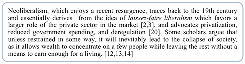
Figure 1. An example of citation in a scientific publication. Note that the examples are all fictitious.
Figure 1 has a segment that reads:
Some scholars argue that unless restrained in some way, it will inevitably lead to the collapse of society, as it allows wealth to concentrate on a few people while leaving the rest without a means to earn enough for a living. [12,13,14]
The goal of (1) is to find out exactly which part of the referred-to papers the author had in mind when putting down the passage. As a further example, consider Figure 2, which has a citing instance,
This is something we call a citing instance or citance (Pocus et al., 1980).
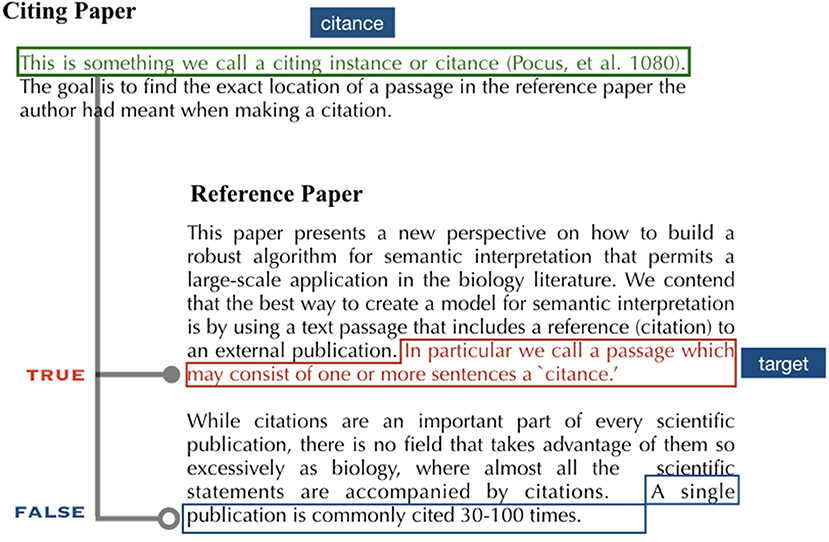
Figure 2. A citance and its target. A sentence boxed in red represents a true target for the citance (one in green box) and one underlined in blue a false target. Note that the examples are all fictitious.
How do we get to its target, marked by the red box in Figure 2? This is a problem the task (1) challenges us to solve.
The results from the task (1) at CL-SciSumm give an overwhelming sense that supervised approaches, in particular, SVMs, are failing to a degree that is almost indistinguishable in performance from a method as simple as TFIDF. In light of this, we turn our attention to neural networks (NNs), which made a huge stride in recent years, to see whether they have any relevance to solving the problem. One particular (much publicized) feature of NNs is that they are an end-to-end system, meaning that they are designed to learn whatever features they need by themselves, freeing humans of the drudgery of making them up. This is something that has not been explored in the previous CL-SciSumm literature, with an exception of Nomoto (2016), who presented a preliminary attempt to leverage neural network to address resolving citation links, from which the current work descends1. One important difference between the earlier and present approach is that the latter takes more seriously how the input is represented, which as we show below, has a huge impact on how well models perform.
Our contribution mainly consists of presenting a novel way to tackle the citation resolution through the application of NNs and identifying some of the operational factors that influence their behavior.
In section 2, we discuss some of the past efforts to capture semantic relatedness among articles, and how they expanded to make use of information that reside outside the text such as citation counts, social relations. Section 3 introduces neural network models. We explain in detail how they actually work to spot potential targets for citations. Sections 5 and 6 will discuss how our approach compares against more conventional baselines, including Ranking-SVM and TFIDF.
2. Related Work
Much of prior work on semantic relatedness among articles focused on exploiting features internal to the text itself such as term frequency, named entity, topical structure, collocation, and burstiness (Lavrenko et al., 2001; Brown, 2002; Chen and Chen, 2002; Chen et al., 2003; Nallapati, 2003; Larkey et al., 2004; Lee and Kageura, 2006; Zhang et al., 2008). Despite a large effort put into research through a project like TDT (Topic Detection and Tracking) (Allen, 2002), a general consensus that emerged out of the experience was that cosine similarity based on TFIDF, simple as it may seem, is the best option, which as it turned out, rivaled or even beat technically more informed approaches. Lavrenko et al. (2001) and Larkey et al. (2004) stand out as an interesting exception with their emphasis on the use of relevance feedback in link detection.
There is another growing trend in the literature, in which people are more concerned about how articles are connected to one another, and try to explain similarity among them through the hyperlink structure (Milne and Witten, 2008; West et al., 2009). Milne and Witten (2008) propose to make use of what they call context terms, or terms in a Wikipedia page likely to serve as an outgoing link, as a part of mechanism to disambiguate word senses. West et al. (2009), meanwhile, seek to enrich the hyperlink structure of Wikipedia by automatically adding links that are useful but left out by humans. A basic idea is to encode a given Wikipedia page in terms of connections it has to the rest of Wikipedia and use the principal component analysis to predict links that are missing from the original structure. Compared to Milne and Witten (2008), which mostly relies on the number of shared links to determine the relatedness of terms, an approach by West et al. (2009) achieves a level of sophistication far beyond that of Milne and Witten (2008).
Among the systems that participated in the 2016 CL-SciSumm conference, those from Cao et al. (2016), Li et al. (2016), and Moraes et al. (2016) are most notable. Cao et al. (2016) split the text into n-sentence long segments and used the SVM Ranking to find a stretch of text likely to be a source of the citation. Moraes et al. (2016) found that an approach using TFIDF together with some preprocessing options (stemming, cutting off sentences that exceed a certain limit) outperformed that based on a tree-kernel. Meanwhile, Li et al. (2016) turned to a rule based model, where they combined diverse similarity metrics (Jaccard, word2vec, idf-based similarity, etc.), each weighted with some hand-picked coefficient, to arrive at a prediction. The approach is manually demanding because how much contribution each feature makes to the final outcome has to be decided by humans, and its ability to generalize is unknown because it was tested only on one particular dataset provided by the CL-SciSumm in 2016.
Despite differences in ways people tackled the problem, a curious commonality emerged from the studies: that a simple similarity metric such as TFIDF or Jaccard works better than those that rely on supervision (Li et al., 2016 even found that Word2Vec fell behind Jaccard). Later in the paper, we will examine whether what they found holds true for the current setup, while looking at how NNs fare against Jaccard and TFIDF.
3. Resolving Citation Links With Neural Networks
In this work, we explore two approaches to modeling citation resolution, both based on neural networks: one is what we might call a “triplet model” which aims to rank sentences in terms of how similar they are to the source sentence (citance); and the other is a binary classification model which labels a given sentence as “true” or “false,” depending on how likely a target it is.
3.1. Triplet Model
We start with the triplet model. Its objective is to provide a scoring function h that favors a true target2 over a false one, or more precisely, to build a function that ensures that h(s, t+) > h(s, t−), where s denotes a citing snippet, t+ denotes a true target (a sentence humans judged as a target) and t− a false target (i.e., a sentence not selected as target). Here and throughout, we assume that both s and t consist of exactly one sentence. If we take Figure 2 as an example, the green box corresponds to s, the red to t+ and the blue to t−
We define h by:
where V(s) denotes a vector derived from s through the application of some neural network and similariy for V(t). One way to ensure that s's similarity with its true target (t+) ranks higher than that with a false target (t−) is to require the following constraint to hold for h (Weston et al., 2010; Bordes et al., 2014):
Noting that we need to ensure that h(s, t−) − h(s, t+) < −C for some constant C (≠ 0), the above formula turns into a loss function:
One way to think about t+ and t− is to take the former as a sentence labeled by humans as a true target and the latter as one of those sentences that are similar to t+ (we call it target-centric supervision as opposed to citance-centric supervision, which we later explain).
Figure 3 gives a general picture of how we move through a neural architecture to C − h(s, t+) + h(s, t−). ψ(·) denotes a representation function that maps a sentence into a discrete or continuous multi-dimensional space. While there are a number of ways to define ψ, we focus on the following three. Note that N is the size of the vocabulary.
(4) represents what is generally known as “word embedding,” where each word in a sentence is assigned to a vector of randomly generated real numbers, whose length I is also arbitrarily chosen (we set I to 10 in the experiments later described). (5) produces a representation that consists of binary values, with 0 indicating the absence and 1 the presence of a particular word in the sentence. (6) works like (5), except that it associates each word with its tfidf value.
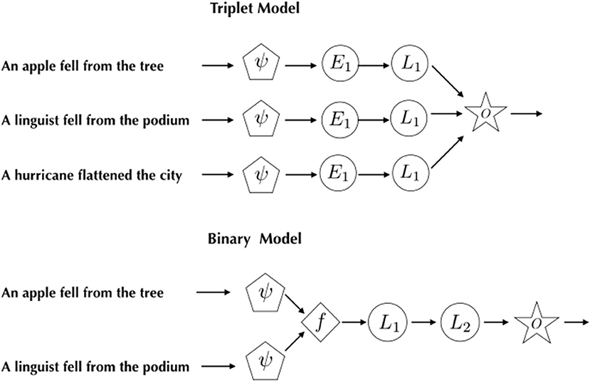
Figure 3. Citation resolution models. ψ is a function to transform the input, mapping it into a matrix of real numbers. f denotes an arithmetic operation on outputs of ψ, L1,2 hidden layers. A star marked with an “O” represents an output layer. The number of hidden units in L1 in the binary model is 100, and that in L2 is 2. L1 in the triplet model consists of 60 hidden units. E1 is an embedding layer containing 10 units.
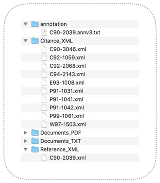
Figure 4. Directory plot of topic cluster C90-2039.
We project ψ(s) and ψ(t) into a hidden layer l via a matrix W (∈ℝN × K)3. K represents the number of neural units in l. Intuitively, one could think of an element of W as indicating the strength of relationship between a word and a corresponding hidden unit. How to determine it is a primary concern of the neural model.
Now we define a layer G1 by
b1 is a parameter for the bias and g an activation function which we take to be a rectifier: i.e., g(x) = max(0, x). For each , we run the stochastic gradient descent (SGD) to minimize:
It is important to note that minimizing has the effect of increasing the chance that the similarity of the citance to its true target is larger than that to a false target. For SGD, we use an optimizer known as ADAM, which makes use of bias corrected moments to adaptively change learning rates (Kingma and Ba, 2015; Ruder, 2016). We set C to 1.0 in the experiments below, following Weston et al. (2013).
3.2. Binary Classification Model
The binary model takes as input a vector of features of the from (f(si1, ti1), …, f(siN, tiN))4, which we feed into the layer G1, whose output is further fed to the following:
The loss function is given by:
where W2 is of the shape K × 2, y is a true label for a given sentence, m is a softmax function. y is assigned to (1, 0) if t is a true target of s and (0, 1), otherwise. We define x · y as an inner product of x and y. We assume f to be either an element-wise multiplication or a squared distance.
4. Data Sets
We created training data from three sources: (1) the “Development-Set-Apr8” dataset (henceforth, DSA2016) (Jaidka et al., 2016); (2) a pilot study corpus which was created as a part of the Text Analysis Conference (TAC2014), prior to DSA2016, and (3) the data made available for the shared task conference at BIRNDL2016 (hereafter, SRD2016). Regardless of where it originates, each dataset contains a number of folders representing a topic, which is composed of one reference paper (RP) and a number of papers that make reference to it (or CPs) 5.
Table 1 give some statistical profiles of TAC2014, DSA2016, and SRD2016. |T| is the number of sentences in RP which CPs' citations are pointing to (target sentences). |RP| represents the number of sentences that comprise the RP, #CPs the number of citing papers, and #Citances the number of citing instances (or citances) in CPs that make reference to RP. |T| tends to be greater than #Citances, as most of target sentences appear in more than one citance.
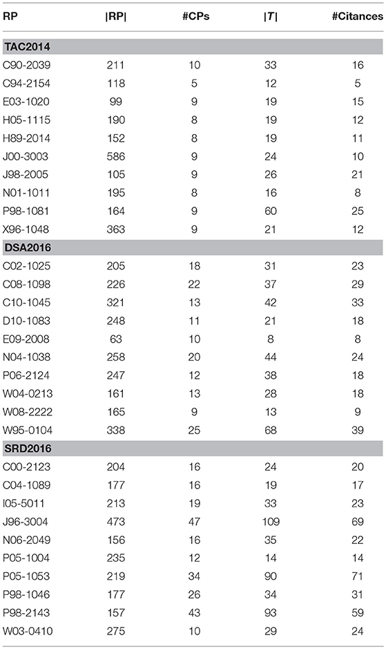
Table 1. Corpus profiles.
In what follows, we mean by ℂℙ a set of sentences that comprise a citing paper and by ℝℙ those that comprise its reference paper. We build a training set by creating a set D of triplets such that: for a given s ∈ ℂℙ and t ∈ ℝℙ,
where R ⊂ ℝℙ. Thus, if we have a reference paper with four sentences {a, b, c, d} a citing instance s from ℂℙ, and a target sentence b, we will have {(s, b, a), (s, b, c), (s, b, d)} as the training data. The size of the training data for topic cluster C roughly sums to:
where r(v) the number of target sentences associated with a citing instance v, and |R| the size of R. 𝕀(C) stands for a set of citing instances in C, a complement of T (a set of target sentences). We set |R| to 10 in the experiments described below.
5. Evaluation
To evaluate, we followed a cross validation style setup where we set aside one cluster for testing, using the rest for training, and report an average performance we get from the validation test on each of the clusters contained in a dataset.
TAC2014, DSA2016, and SRD2016 each came with ten topic clusters, consisting of one reference paper and a number of papers which cite that paper. We gauged performance by a metric known as MRR (mean reciprocal rank), which produces the average of the inverted ranks of first true targets retrieved by the models. The closer an MRR is to 1, the better the performance is. Formally, MRR is defined as
C is a set of citances (see Figure 5 for an example) and M a model6. In case a citance or a target involves multiple sentences, we split them into pairs of sentences in such a way that each pair will consist of exactly one sentence from s and one from t. This makes it easier for NNs to handle inputs, as they require that the length of input to stay fixed. rankM(t[i]) represents the rank of the first true target returned by M for the i-th citance. Note that MRR is meant to measure performance not in terms of how similar the output is to target sentences as was done in the past SciSumm events, but in terms of how accurately we locate a true target. We believe this is more in line with the goal of the CL-SciSumm7, 8.
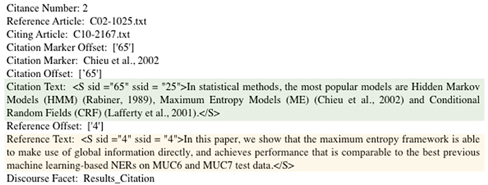
Figure 5. Citation and target. A 65th sentence in C10-2167 is seen as referring to a fourth sentence in C02-1025.
To find how neural models compare to some of the more conventional methods, we also included Ranking SVM (SVR, henceforth) (Joachims, 2006)9 in a roster of models we put to the test. As mentioned earlier, given the relative paucity of positive instances available, it may be hard to get a meaningful insight by running a discriminatory version of SVM, as it requires a sizable amount of training data for each of the labels we are interested in. Since we have on the average, positive instances accounting for only about 10% of the corpus amenable to use in training, the discrete classification with SVM is a non starter. This is the reason we turn to SVR.
Preliminary tests we ran on NNs found that NNs trained on triplets created with the target-centric supervision (section 3.1) were not able to produce performance on a par with baselines. Which promoted us to come up with an alternative setup, where we regard sentences in ℝℙ that are most similar to those in ℂℙ as targets, entirely dismissing the annotations supplied by humans (which we call citance-centric supervision or CCS)10. As it turned out, the adoption of CCS brought a clear gain to NNs, propelling them over baselines by a comfortable margin.
Under the new setup, we have a triplet of the form:
where t is a sentence in ℝℙ that ranks between the 1st and 10th in terms of the similarity to s (∈ℂℙ) and u (∈ℝℙ) is a sentence that ranks between the 11th and 20th (the similarity was given in the dot-product). n is the number of training instances. We also applied the idea to the binary classification model: we treated top 10 most similar sentences as true targets and those that did not make it to the top 10 but ranked above 21 as corrupt or false. The training and test data for the binary classifier look like:
ψ is either ψb or ψt. f is an element-wise multiplication or a squared distance. y ∈ {1, 0}. s ∈ ℂℙ and t ∈ ℝℙ. SVR was trained on D2 with f set to the element-wise multiplication.
In addition to SVR, we consider two other baselines, TFIDF and BDOT Both make use of the inner product to determine whether t is a target for s. They differ only in what they take as input: TFIDF operates on vectors of values expressed in TFIDF, while BDOT on those that consist of binary values. Formally, they will come to:
Notice that BDOT is in practice equivalent to a familiar Jaccard coefficient:
which the previous literature found to be singularly effective for identifying the target passage (Li et al., 2016). In BDOT, we can safely ignore the denominator as it remains invariant: |ψb(s) ∪ ψb(t)| = N (the size of the vocabulary, i.e., the number of unique tokens that comprise the dataset).
Finding MRR involves ranking for a given s ∈ ℂℙ, a sentence t in ℝℙ in accordance to how similar s is to t. For SVR, TFIDF, and BDOT, this is straightforward. For NNs, however, things get somewhat tricky, as their outputs represent the loss, not the similarity. So we use G1 instead [see (7)] as an indicator of the strength of the relationship between s and t: in other words, we quantify the similarity by .
Moreover, to get a broad picture of how the models perform, we introduce an idea we call approximately correct targets (ACTs), where we are not only interested in finding out whether they pick up exact sentences humans labeled as true targets, but also finding out how close predictions are to the true targets.
Consider Figure 6. A target sentence of interest is one circled in red. We mean by approximately correct targets, those sentences that appear n sentences away (both forward and backward) from the target, where n is arbitrarily chosen (which is set at 3 in the example) and take any sentence that occurs within the region to be as correct as the true target. In Figure 6, ACTs are found in the area shaded in light blue. A motivation for this idea comes from our curiosity to find out whether it is possible to achieve meaningful performance by making the citation resolution less hard (the preliminary experiments suggest it will not happen if we stick to the strict target span).
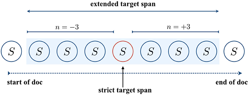
Figure 6. Strict vs. extended target span.
6. Results and Discussion
Tables 2, 3 show the outcome of running NNs in four different setups, along with baselines11. “NN: in = binary,loss = entropy” refers to a binary classification model using ψb for the input transformation, and the L2 loss function. “NN: in = binary, loss = triplet” denotes a triplet model with ψb for the input and the loss measured in L1. “NN: in = tfidf, loss = triplet” and “NN: in = embedding, loss = triplet” are like the previous model except that the former uses ψt and the latter, ψe in place of ψb. The top row indicates the length of the target span. For instance, n = ±3 means that any of the three sentences that either precede or follow the target sentence is considered ACTs; and n = ±0 means that there is no ACT other than the target sentence itself.
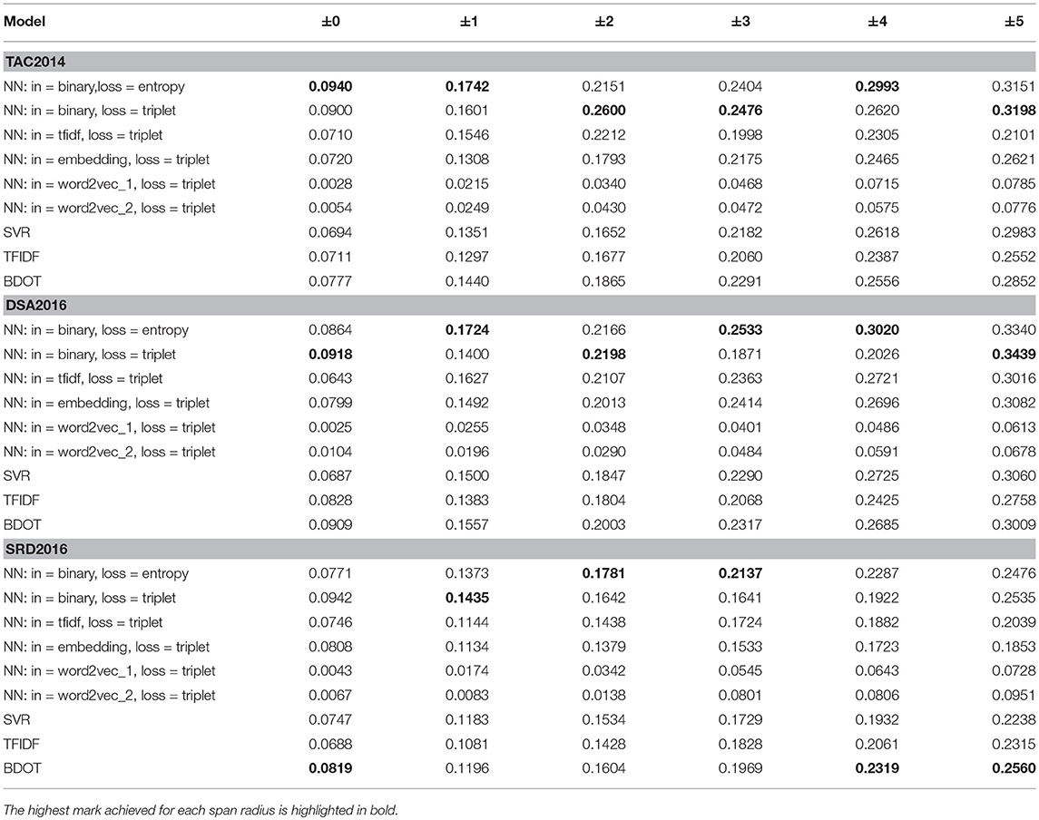
Table 2. Results in MRR for CCS.
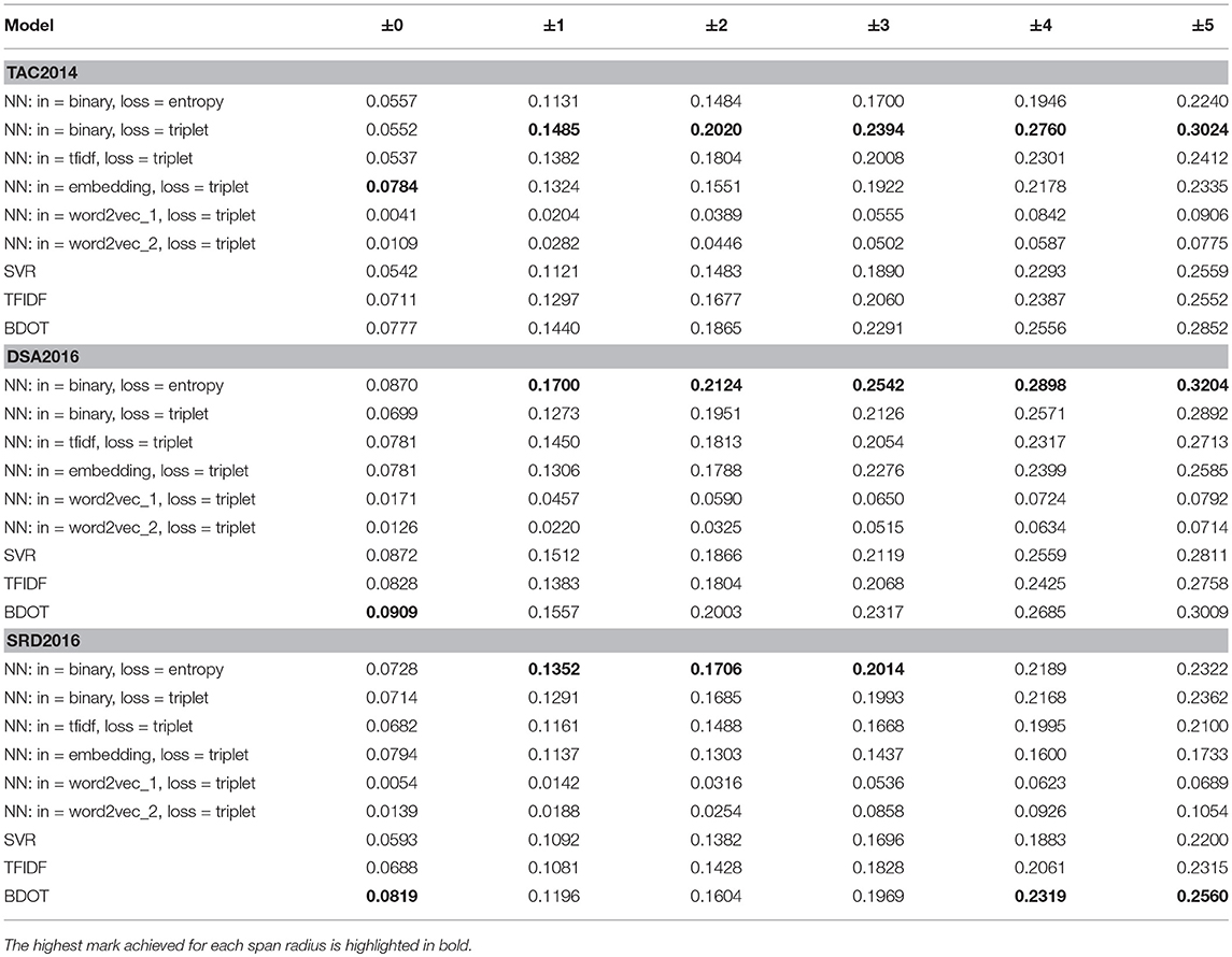
Table 3. Results in MRR for TCS.
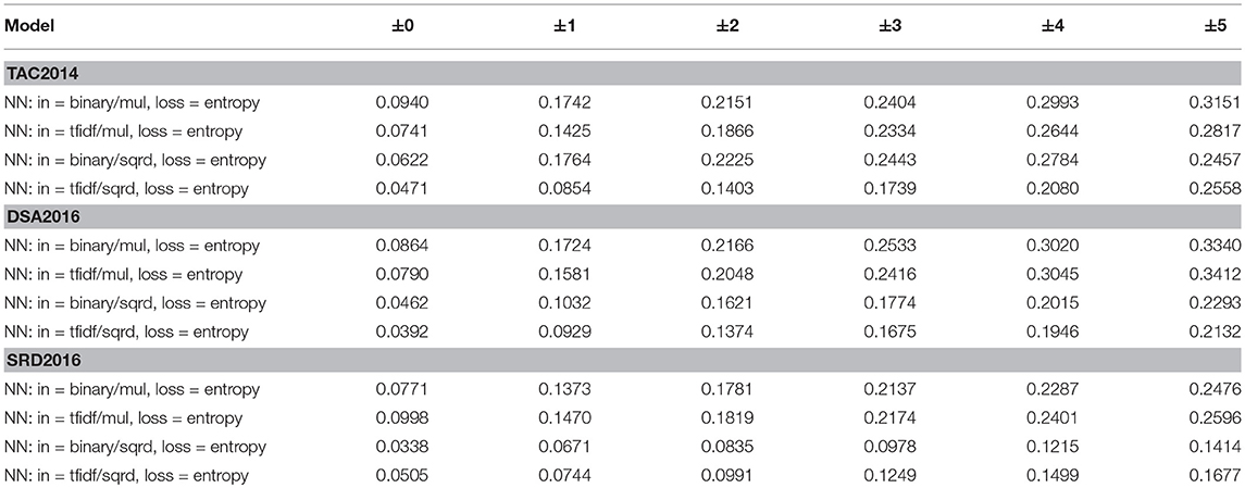
Table 4. Effects of multiplication vs. squared distance on performance.
The numbers in the tables show MRRs averaged over 10 topic clusters (An MRR for each cluster was produced via a by-topic cross validation, where we set aside one topic cluster for testing and use the rest for training).
6.1. CCS vs. TCS
The results in CCS or citance-centric supervision (Table 2) show a clear tendency for the NNs to score higher than the baselines, which include SVR, TFIDF, and BDOT, across varying lengths of the span. Of a particular note is the performance of models which take the input in binary format, against those that employ TFIDF or the embedding12. We see the former consistently outperforming the latter. It is safe to say that representing the input in binary format led to the superior performance, which parallels BDOT outperforming TFIDF across the datasets.
By contrast, in TCS (target-centric supervision), NNs suffer an across-the-board decline in performance, with some of the top performers under CCS dipping below baselines. It is interesting that they seem to suffer more in TAC than in DSA and SRD, which could be attributable to the fact that TAC contains less citing papers than the other two (cf. Table 1). Yet the triplet model still performs better on inputs represented in binary format than on those in tfidf, which echoes what we found in CCS.
The finding that CCS yields a better performance happen than TCS regardless of models we choose, is signficant. Because what it implies is that hand created annotations are no better than those created automatically by using a simple similarity metric (or L1-norm in our case), in terms of quality they permit as training data. To further investigate the matter, we examined whether the performance we see under CCS is significantly different from that we have under TCS. The results are shown in Table 5. We see “NN: in = binary, loss = entropy” having 0.0006⋆ for p-value, meaning that the performance it had in CCS was significantly different from results it produced in TCS. So there appear to be some grounds for arguing that whether one works with CCS or TCS does have consequences for neural models, though how much the choice affects them varies from model to model. “NN: in = binary, loss = entropy” tends to be more sensitive to the choice. The same appears to be the case with models involving an embedding of one sort or another. In constrast, “NN: in = binary, loss = triplet” is totally blind to whatever differences there might be between the two modes of annotation. Yet the fact that CCS in general leads to better results, some of which we found to be statistically different from those under TCS, does cast some doubt over the rationale of using human created annotations as gold standards. Whether this is due to a particular way the datasets were created or to difficulties inherent to annotating papers for citation links, remains to be seen.
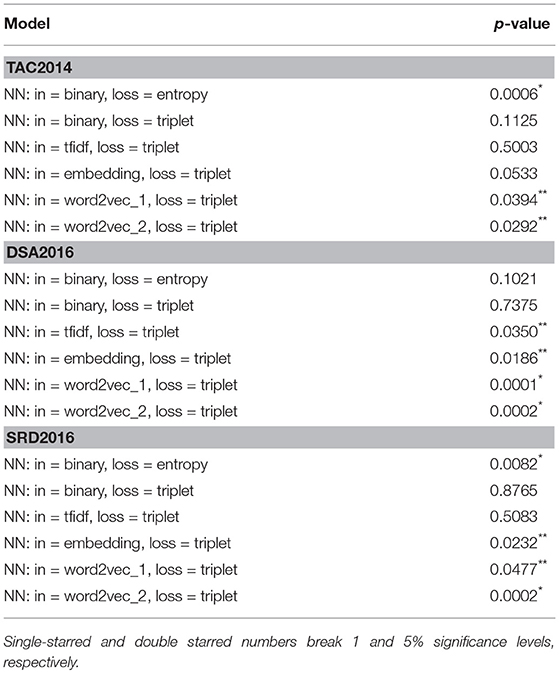
Table 5. Significance Test of CCS against TCS (with paired t-test).
6.2. Word2Vec Models
Meanwhile, being somewhat struck by a unremarkable performance of the embedding model, we decided to explore the use of a pre-trained embedding model based on Word2Vec, which recently has proven its utility across a wide range of NLP tasks. Word2Vec is a single layer neural network whose primary goal is to predict a given word using its left and right contexts (CBOW) or words that occur closely to what is given as an input (Skip-Gram). Its importance lies not in its ability to predict missing words per se, but in the implication that a hidden structure built while training the model can be used as a latent “semantic” representation of word. To determine its utility in the current context, we did experiments with two versions of Word2Vec, one based on the Google News corpus (word2vec_1) 13, and the other built from the training data (word2vec_2). In either case, we made use of the Skip-Gram variant of Word2Vec (the latter model was trained with GENSIM14). We set the length of a hidden layer to 300, both for the version that employs the Google News and the one we created locally. The results are found in Tables 2, 3.
Faced with the way they turned out, which was as underwhelming as the non-Word2Vec embedding model we saw previously, we came to a conclusion that the semantics may have little relevance to predicting target passages. The unimpressive performance of the embedding models stands in sharp contrast to the binary models, which rely only on the superficial overlap between source and target sentences to produce a more decent performance. The fact that BDOT—which looks at the amount of tokens shared among the source and target to determine where the citation comes from—is closing in on the binary models lends a further support for the idea that a superficial match is a more reliable indicator of the target than the semantics served by the embedding models. Remarkably, the finding is consonant with what Li et al. (2016) found in their ablation study, who observed that Jaccard coefficient was by far the most effective feature among those they considered, including Word2Vec.
6.3. Factors Influencing MRRs
In light of the discussion so far, it would be interesting to ask whether there is any feature of the dataset that affects the models' performance. Table 6 gives some insights, which lists the result of regressing MRR on features that we used previously to describe each dataset, namely, |RP|, CP, |T|, and |C|, where statistically significant features are noted with usual markings. It shows clearly that |RP|, the length of the reference paper is a single most significant predictor of the model's performance. In other words, the shorter the reference, the better the outcome. It turns out that neither the number of CPs nor that of targets is nearly as predictive as the length of RP.
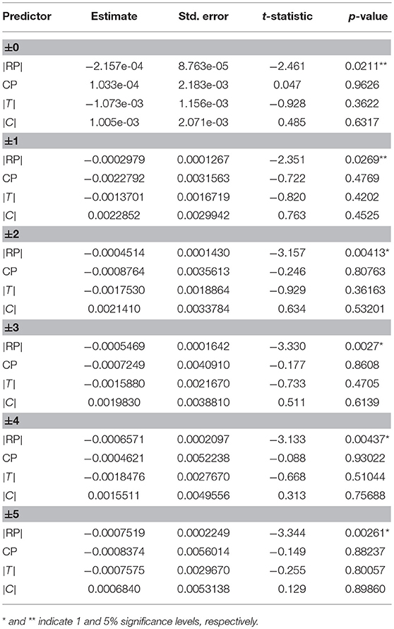
Table 6. An analysis on how much individual cluster features affect the task performance, based on a multiple linear regression (where MRR is regressed on |RP|, CP, |T| and |C| at each span radius).
In the meantime, Table 4 looks at whether the choice for f has any effect on performance of the binary model. “mul” indicates the element-wise multiplication and “sqrd” the squared distance. The results clearly indicate that “mul” is a better choice, regardless of how the input is represented. Why this is so, is a curious question. One hypothesis is that the multiplication over binary inputs has the effect of eliminating all the words which occur only in s or t, which somehow caused some useful patterns to emerge, which NNs exploited. Though it is not clear at this time where the truth lies, a general lesson one might draw from the experiments is that how the inputs are encoded is at least as important as how the models are configured and some careful thinking must go into designing how to express what one feeds into NNs.
6.4. Summary of Findings
We conclude the section by highlighting some of the key findings from the experiments.
• Semantic representation: the token-wise overlap (BDOT/Jaccard) is a stronger indicator of a target than the implicit semantic representation induced via the embedding or Word2Vec (Note that by the embedding, we mean a random projection of a word into a continuous space, which obviously is distinct from a Word2Vec induced representation, as the latter is constructed using weights (associated with a particular layer) that Word2Vec learned during the training).
• CCS (automatic annotation) vs. TCS (manual annotation): we found statistically significant differences between CCS and TCS in terms of how they impact the performance, though how much susceptible models are to the differences varies from one model to another. “NN: in = binary, loss = triplet” benefitted more from a shift from TCS to CCS, compared to other models.
• Cross-entropy vs. triplet loss: there is a tendency for the former to result in a superior performance over the latter.
Before leaving the section, as a way to assist the reader with an intuitive understanding of what differences and similarities lie among the topic clusters, we provide in Figure 7 plots of by-topic performance (in CCS) of “NN: in = binary, loss = entropy” on each of the relevant datasets.
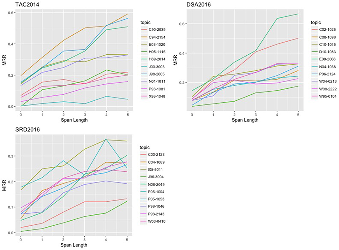
Figure 7. Plot of by-topic performance of NN:binary+entropy.
7. Conclusions
We have presented approaches to linking citation and reference that draw upon neural networks (NNs), and described in detail what machinery is involved and what we found in experiments with the three datasets, TAC2014, DSA2016, and SRD2016. We introduced the notion of approximately correct targets, an idea that we should treat sentences that occur in the vicinity of true targets as equally correct, whereby we try to identify an area which is likely to include a true target, instead of finding its exact location. The experiments found that expanding the target region by 5 sentences in radius led to a four fold increase in MRR across the models. Another curious fact the experiments brought to light was the significance of the way the input is expressed: it turned out that NNs worked visibly better with the binary representation than with either TFIDF or embeddings of the sort we considered in this paper. Also worthy of some attention is a finding that dispensing human created labels altogether led to an improvement (recall discussion on target- vs. citance-centric labeling). How it is so is an interesting question we have yet to answer. The paucity of human annotations, and the lack of consistent patterns in human labelings are some of the possible causes that immediately come to mind. To fully answer the question, however, may require finding out how well humans agree on their judgments as well as collecting additional data, topics we will leave to the future research.
Author Contributions
The author confirms that he is the sole contributor of the present work and responsible for any error and misrepresentation thereof.
Conflict of Interest Statement
The author declares that the research was conducted in the absence of any commercial or financial relationships that could be construed as a potential conflict of interest.
Footnotes
1. ^Some of the NNs we develop here are an adaptation of the embedding models proposed by Weston et al. (2010, 2013) and Bordes et al. (2013, 2014).
2. ^By target, we mean one or more sentence in the referred-to paper (RP) that serve as a source for a snippet or text citing the RP: for example, a sentence boxed in red in Figure 2; and those not boxed are said to be false targets with respect to the citance.
3. ^Note that the shape of W will become I times N by K, when working with word embedding. As a further note, ψb(s) is of shape S × N, where S is the length of sentence s (the number of words) and N the size of the vocabulary, with each word represented as a “one-hot” vector, meaning it consists of a single vector of size N, with all cells set to 0, except for one that corresponds to the relevant word, which is set to 1. ψt(s) works the same way, except that each word vector has a tfidf value where ψb(s) has 1.
4. ^sij denotes the j-th word in the vocabulary that appears in si. The same applies to tij.
5. ^Figure 4 shows one such cluster: what appears under Citance_XML is a group of papers that contain passages (citances) that refer to paper C90-2039, which is placed in a directory called Reference_XML. The former corresponds to CPs and the latter to RP. Associated with each topic cluster is a file that contains human created annotations (e.g., C90-2039-annv3.txt in Figure 4) that indicate which part of the RP a given citing passage relates to, an example of which is found in Figure 5: the area shaded in green contains information on a citing passage and the one in yellow indicates a target sentence.
6. ^It is safe to assume that a ground truth citance consists of two types of information: the site of a citing instance in ℂℙ and that of its target in ℝℙ.
7. ^We were told that they abandoned an accuracy based metric because it was not able to distinguish participating systems, with their performance crawling around 0.
8. ^While a particular way we set up the evaluation makes it infeasible to make a direct comparison to the systems at the CL-SciSumm, we included in the evaluation, our analogs of baselines that were noted at the conference for their strong performance over other competing methods, in particular, TFIDF, Jaccard, and SVM-Ranking, which would provide some sense of how the current setup compares to the previous approaches.
9. ^We used the sklearn library to implement the SVR (http://scikit-learn.org/stable/modules/generated/sklearn.svm.SVR.html).
10. ^This is equivalent to what is generally known as distant supervision in the machine learning literature, where training labels are created artificially with heuristics or rules (cf. Mintz et al., 2009).
11. ^We performed stemming and removed stop words, using the NLTK package (Bird et al., 2009). All the NNs described here were created using the tensorflow package (https://www.tensorflow.org).
12. ^The statement here is not meant to suggest that any form of embedding will meet the same fate.
13. ^GoogleNews-vectors-negative300.bin.gz (https://github.com/mmihaltz/word2vec-GoogleNews-vectors.git).
References
Allen, J. (ed.). (2002). Topic Detection and Tracking: Event-Based Information Organization. Dordrecht: Kluwer Academic Publishers.
Bethard, S., and Jurafsky, D. (2010). “Who should i cite: learning literature search models from citation behavior,” in Proceedings of the 19th ACM International Conference on Information and Knowledge Management (New York, NY: ACM), 609–618. doi: 10.1145/1871437.1871517
Bird, S., Klein, E., and Loper, E. (2009). Natural Language Processing with Python. Sebastopol, CA: O'Reilly Media Inc.
Bordes, A., Usunier, N., Weston, J., and Yakhnenko, O. (2013). “Translating embeddings for modeling multi-relational data,” in Advances in Neural Information Processing Systems (Lake Tahoe, CA), 1–9.
Bordes, A., Weston, J., and Usunier, N. (2014). “Open question answering with weakly supervised embedding models,” in ECML PKDD 2014 (Nancy).
Brown, R. (2002). “Dynamic stopwording for story link detection,” in Proceedings of HLT 2002: Second International Conference on Human Language Technology (San Diego, CA), 190–193.
Cao, Z., Li, W., and Wu, D. (2016). “Polyu at cl-scisumm 2016,” in BIRNDL 2016 Joint Workshop on Bibliometric-enhanced Information Retrieval and NLP for Digital Libraries (Newark, NJ), 132–138.
Chen, F., Farahat, A., and Brants, T. (2003). “Story link detection and new event detection are asymmetric,” in Proceedings of HLT-NACCL 2003 (Edmonton), 13–15.
Chen, Y.-J., and Chen, H.-H. (2002). “NLP and IR approaches to monolingual and multilingual link dectection,” in The 19th International Conference on Computational Linguistics (COLING-2002) (Taipei).
Jaidka, K., Chandrasekaran, M. K., Rustagi, S., and Kan, M.-Y. (2016). “Overview of the 2nd computational linguistics scientific document summarization shared task (cl-scisumm 2016),” in The Proceedings of the Joint Workshop on Bibliometric-enhanced Information Retrieval and Natural Language Processing for Digital Libraries (BIRNDL 2016) (Newark, NJ).
Joachims, T. (2006). “Training linear SVMs in linear time,” in Proceedings of the ACM Conference on Knowledge Discovery and Data Mining (KDD) (Philadelphia, PA).
Kingma, D., and Ba, J. L. (2015). “Adam: a method for stochastic optimization,” in Proceedings of the International Conference on Learning Representation (San Diego, CA), 1–13.
Larkey, L. S., Feng, F., Connell, M., and Lavrenko, V. (2004). “Language-specific models in multilingual topic tracking,” in SIGIR '04: Proceedings of the 27th Annual International ACM SIGIR Conference on Research and Development in Information Retrieval (New York, NY: ACM), 402–409.
Lavrenko, V., DeGuzman, J. A. E., LaFallme, D., Pollard, V., and Thomas, S. (2001). “Relevance models for topic detection and tracking,” in Proceedings of the Conference on Human Language Technology (Stroudsburg, PA), 102–110.
Lee, K.-S., and Kageura, K. (2006). Korean-Japanese story link detection based on distributional and contrastive properties of event terms. Inform. Process. Manage. 42, 538–550. doi: 10.1016/j.ipm.2005.02.005
Li, L., Mao, L., Zhang, Y., Chi, J., Huang, T., and Heng Peng, X. C. (2016). “Cist system for cl-scisumm 2016 shared task,” in BIRNDL 2016 Joint Workshop on Bibliometric-Enhanced Information Retrieval and NLP for Digital Libraries (Newark, NJ), 156–166.
Meij, E., and de Rijke, M. (2007). “Using prior information from citataions in literature search,” in Proceedings of RIAO2007 (Pittsburgh, PA).
Milne, D., and Witten, I. H. (2008). “Learning to link with wikipedia,” in Proceedings of the 17th ACM Conference on Information and Knowledge Management (New York, NY: ACM), 509–518. doi: 10.1145/1458082.1458150
Mintz, M., Bills, S., Snow, R., and Jurafsky, D. (2009). “Distant supervision for relation extraction without labeled data,” in Proceedings of the Joint Conference of the 47th Annual Meeting of the ACL and the 4th International Joint Conference on Natural Language Processing of the AFNLP: Volume 2 - Volume 2 (Stroudsburg, PA: Association for Computational Linguistics), 1003–1011.
Moraes, L., Baki, S., Verma, R., and Lee, D. (2016). “University of houston at cl-scisumm 2016: Svms with tree kernels and sentence similarity,” in BIRNDL 2016 Joint Workshop on Bibliometric-Enhanced Information Retrieval and NLP for Digital Libraries (Newark, NJ), 113–121.
Nallapati, R. (2003). “Semantic language models for topic detection and tracking,” in Proceedings of the HLT-NAACL 2003 Student Research Workshop (Edmonton), 1–6.
Nomoto, T. (2016). “NEAL:a neurally enhanced approach to linking citation and reference,” in The Proceedings of the Joint Workshop on Bibliometric-enhanced Information Retrieval and Natural Language Processing for Digital Libraries (Newark, NJ).
Ruder, S. (2016). An overview of gradient descent optimisation algorithms. arxiv preprint arxiv:1609.04747.
West, R., Precup, D., and Pineau, J. (2009). “Completing wikipedia's hyperlink structure through dimensionality reduction,” in Proceedings of the 18th ACM Conference on Information and Knowledge Management (New York, NY: ACM), 1097–1106. doi: 10.1145/1645953.1646093
Weston, J., Bengio, S., and Usunier, N. (2010). Large scale image annotation: Learning to rank with joint word-image embeddings. Mach. Learn. 81, 21–35. doi: 10.1007/s10994-010-5198-3
Weston, J., Bordes, A., Yakhnenko, O., and Usunier, N. (2013). “Connecting language and knowledge bases with embedding models for relation extraction,” in Empirical Methods in Natural Language Processing (Seattle, WA), 1366–1371.
Keywords: neural network model, citation resolution, text similarity, ACL anthology, machine learning, natural language processing
Citation: Nomoto T (2018) Resolving Citation Links With Neural Networks. Front. Res. Metr. Anal. 3:31. doi: 10.3389/frma.2018.00031
Received: 29 January 2018; Accepted: 12 September 2018;
Published: 25 October 2018.
Edited by:
Philipp Mayr, Leibniz Institut für Sozialwissenschaften (GESIS), GermanyReviewed by:
Haozhen Zhao, Navigant, United StatesMuthu Kumar Chandrasekaran, National University of Singapore, Singapore
Copyright © 2018 Nomoto. This is an open-access article distributed under the terms of the Creative Commons Attribution License (CC BY). The use, distribution or reproduction in other forums is permitted, provided the original author(s) and the copyright owner(s) are credited and that the original publication in this journal is cited, in accordance with accepted academic practice. No use, distribution or reproduction is permitted which does not comply with these terms.
*Correspondence: Tadashi Nomoto, bm9tb3RvQGFjbS5vcmc=