Extraction of Hierarchical Behavior Patterns Using a Non-parametric Bayesian Approach

Extraction of complex temporal patterns, such as human behaviors, from time series data is a challenging yet important problem. The double articulation analyzer has been previously proposed by Taniguchi et al. to discover a hierarchical structure that leads to complex temporal patterns. It segments time series into hierarchical state subsequences, with the higher level and the lower level analogous to words and phonemes, respectively. The double articulation analyzer approximates the sequences in the lower level by linear functions. However, it is not suitable to model real behaviors since such a linear function is too simple to represent their non-linearity even after the segmentation. Thus, we propose a new method that models the lower segments by fitting autoregressive functions that allows for more complex dynamics, and discovers a hierarchical structure based on these dynamics. To achieve this goal, we propose a method that integrates the beta process—autoregressive hidden Markov model and the double articulation by nested Pitman-Yor language model. Our results showed that the proposed method extracted temporal patterns in both low and high levels from synthesized datasets and a motion capture dataset with smaller errors than those of the double articulation analyzer.

1. Introduction

In the big data era, we can easily collect information-rich time series thanks to the advancements in sensing technologies. However, such time series data are not segmented and hence difficult to apply recent machine learning techniques. To segment such data, extraction of temporal patterns in an unsupervised manner is necessary. This has become an active topic in several research fields, such as health care (Zeger et al., 2006), biology (Saeedi et al., 2016), speech recognition (Taniguchi et al., 2016), natural language processing (Heller et al., 2009), and motion analysis (Barbič et al., 2004). Although many methods have been proposed to extract temporal patterns (Keogh et al., 2004), there exists a problem that the number of existing patterns (and consequently, the number of segments) is generally unknown beforehand. To solve this issue, non-parametric Bayesian methods are used to determine the number of patterns (Fox et al., 2008b). Specifically, non-parametric Bayesian methods based on switching AR models, such as the beta process—autoregressive hidden Markov model (BP-AR-HMM) (Fox et al., 2009, 2014), can be used to identify the temporal patterns without specifying the number of patterns beforehand.

Although conventional methods can discover the temporal patterns to segment a time-series sequence, some sequences have a hierarchical structure that makes the segmentation more complex. Motion data, for example, can be seen as a sequence of semantic actions, where each action can be decomposed as a series of motion primitives (Viviani and Cenzato, 1985; Zhou et al., 2013; Grigore and Scassellati, 2017). Similarly, speech data consist of words, where each word consists of phonemes. With such a hierarchical structure, usual methods involving switching dynamical systems may not be sufficient since they do not assume the existence of the hierarchical structure. Time series sequences like the examples above should then be analyzed using hierarchical models. Non-parametric Bayesian methods for hierarchical models include the hierarchical hidden Markov model (HHMM) (Fine et al., 1998), the nested Pitman-Yor language model (NPYLM) for sentences (Mochihashi et al., 2009), and the double articulation analyzer (DAA) (Taniguchi and Nagasaka, 2011). However, they are not suitable for analyzing the dynamic patterns. For example, DAA only modeled the time series sequences by fitting segment-wise linear functions to the lower level of the structure. Complex dynamics in the lower level has not been considered in the previous method, despite motion primitives being usually modeled as non-linear functions (Williams et al., 2007; Bruno et al., 2012).

From these backgrounds, it is necessary to develop a method that considers both dynamics and hierarchical structure to extract temporal patterns. To realize such a method, we naively applied BP-AR-HMM and NPYLM in order to model hierarchically-structured sequences with dynamical systems in our previous study (Briones et al., 2018).

In this work, we propose a model that integrates BP-AR-HMM and NPYLM as a unified model. Our method can capture the hierarchical structure of the time series by NPYLM and use dynamical systems (specifically, switching AR models in BP-AR-HMM) to represent the dynamic pattern in the lower level sequences. Also, BP-AR-HMM allows for asynchronous switching of segments across the multiple time series data considered thanks to the beta process in BP-AR-HMM. Compared to our previous two-step approach, the proposed integrated approach is expected to improve segmentation and estimation accuracy. In this study, we tested our method with toy dataset and sequences generated from real motion capture (mocap) sequences with two interacting agents. Such motion sequences are suitable to test the segmentation performance of our method, since interaction switches from time to time (Ryoo and Aggarwal, 2009; Alazrai et al., 2015).

The rest of this paper is organized as follows: section 2 shows our proposed method, with a brief introduction of basic algorithms. Sections 3 and 4 outline the details of the synthetic experiments carried out using two datasets and their corresponding results. Finally, section 5 gives some discussion of the results, including the conclusions.

2. Proposed Method

We propose to use a hierarchical non-parametric Bayesian approach to extract hierarchical temporal patterns from time series data. Specifically, we use an unsupervised segmentation method, where the extracted segments are used to define the temporal patterns. Our method consists of two non-parametric Bayesian models: BP-AR-HMM (Fox et al., 2009) and NPYLM (Mochihashi et al., 2009) (Figure 1).

FIGURE 1

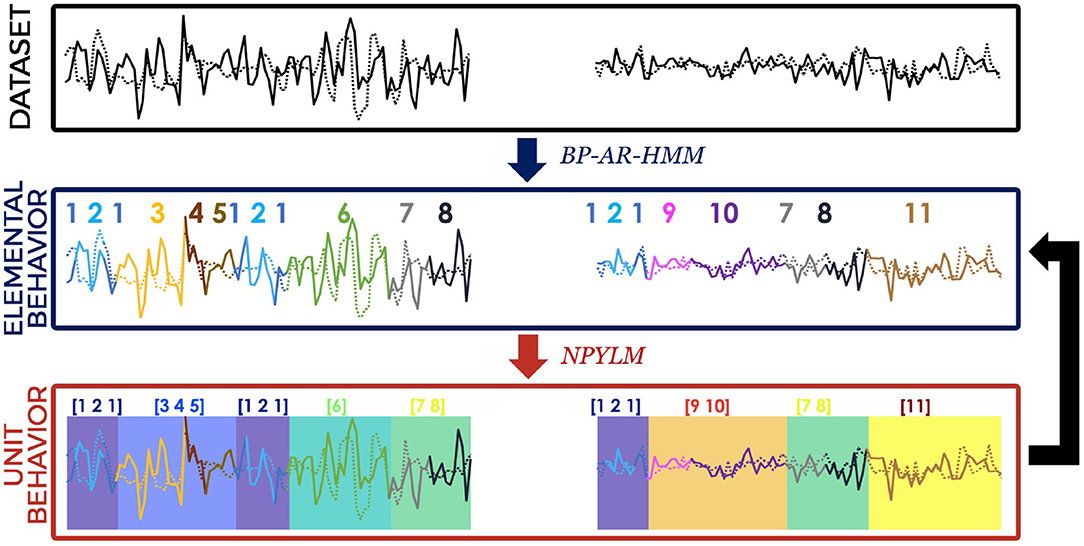
Figure 1. Illustration of processing steps in our proposed method. Each time step is assigned both an EB label (line color) and UB label (background color). The summarized sequence of EB labels (shown as numbers above the lines) obtained from BP-AR-HMM are then grouped together (indicated by the square brackets) using NPYLM.

In the first step, BP-AR-HMM is applied to time series data, to discover low-level temporal patterns or elemental behaviors (EB), which correspond to the motion primitives in the motion analysis. Segmentation is indicated by assigning EB labels at each time step. The obtained EB label sequences for each time series are then summarized, before being used as an input for the second step. In the second step, NPYLM is applied to the (summarized) sequence of EB labels, to detect unit behaviors (UB). Subsequences of EB labels with recurring patterns are grouped together and assigned UB labels. As a consequence, the method outputs a sequence of UBs, each of which is a sequence of EBs represented by AR models. Then, these two steps are iterated a fixed number of times, with the resulting UB labels from the NPYLM step used as initial EB labels for the BP-AR-HMM step of the next iteration.

In the following, we introduce the components of our method: BP-AR-HMM and NPYLM.

2.1. BP-AR-HMM

BP-AR-HMM is an extension of hidden Markov model where each discrete latent variable z_t has an AR model of order r with parameter θ_zt = {A_zt, Σ_zt} (Figure 2), and the observed variable y_t is represented as an AR model with lag order r. This model is a non-parametric Bayesian model with a beta process prior, where an indicator vector over the set of EBs, f_i, is drawn. The EB z_t, the state transition matrix ${\pi }_j^{(i)}$, and the AR coefficient matrix A_k are drawn according to f_i, a gamma prior, and a matrix normal prior, respectively (Figure 2).

FIGURE 2

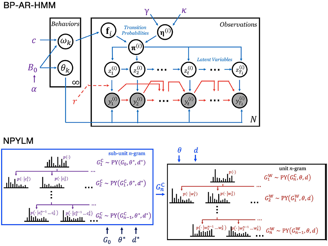
Figure 2. Graphical representations of the non-parametric Bayesian models. (Top) BP-AR-HMM. (Bottom) NPYLM.

2.1.1. Beta Process (BP)

A beta process prior is placed on the EB indicator vector. This makes it possible to not specify the number of EBs beforehand, and thus allow us to use an infinite-dimensional EB indicator vector f. A beta process is a completely random measure, denoted by

$\begin{array}{ll}B|c,B_0~\text{BP}(c,B_0),& (1)\end{array}$

$\begin{array}{llll}B& =& {\displaystyle \sum _{k=1}^{\infty }}{\omega }_k{\delta }_{{\theta }_k},\text{ with }\alpha =B_0(\Theta ),& (2)\end{array}$

where B₀ is a base measure, c the concentration parameter, and α the mass parameter. The number of active EBs, including which EBs are active, for time series i is determined by a realization of the indicator vector f_i | B~BeP(B), given by

$\begin{array}{ll}{\text{f}}_i={\displaystyle \sum _k}{f}_{ik}{\delta }_{{\theta }_k},\text{ with }{f}_{ik}~\text{Be }({\omega }_k).& (3)\end{array}$

Here, f_ik = 1 if the kth EB is active for time series i, i = 1, …N.

2.1.2. AR-HMM

The D-dimensional observation vector y_t is described by an autoregressive hidden Markov model (AR-HMM), with order r, latent variable (state sequences) z_t, and transition probability matrix π_k. That is,

$\begin{array}{ll}{z}_t|z_{t-1}~{\pi }_{z_{t-1}},& (4)\end{array}$

$\begin{array}{ll}{\text{y}}_t|z_t~{N}({\text{A}}_{z_t}{\tilde{\text{y}}}_t,{\Sigma }_{z_t}),& (5)\end{array}$

$\begin{array}{ll}{\text{y}}_t={\displaystyle \sum _{l=1}^r}{A}_{l,z_t}{\text{y}}_{t-l}+{\text{e}}_t(z_t),\text{with }{\text{e}}_t(z_t)~{N}(0,{\Sigma }_{z_t})& (6)\end{array}$

For the kth EB, the corresponding AR-HMM parameters are denoted as θ_k = {A_k, Σ_k}, while the transition probabilities are denoted by π_k. Since active EBs vary for each sequence, feature-constrained transition distributions (Fox et al., 2009) are used. That is, given f_i,

$\begin{array}{l}{\pi }_{kj}^{(i)}=\{\begin{array}{ll}0& f_{ij}=0\\ P\left(z_t^{(i)}=j|z_{t-1}^{(i)}=k\right)& f_{ij}=1\\ \end{array},\\ \text{ with}{\displaystyle \sum _j}{\pi }_{kj}^{(i)}=1.& (7)\end{array}$

A gamma prior would be placed on the transition matrix, with

$\begin{array}{ll}{\eta }_{jk}|\gamma ,\kappa ~\text{Gamma}(\gamma +\kappa {\delta }_{j,k},1),& (8)\end{array}$

$\begin{array}{ll}{\pi }_j^{(i)}=\frac{{\eta }_j^{(i)}\otimes {\text{f}}_i}{{\displaystyle {\sum }_{k|f_{ik}=1}}{\eta }_{jk}^{(i)}},& (9)\end{array}$

where γ, κ are the transition and transition sticky parameter, respectively. Moreover, δ_{j, k} is the Kronecker delta function, and ⊗ is the Hadamard (or element-wise) vector product.

Moreover, matrix normal priors would be placed on the dynamic parameters. That is,

$\begin{array}{ll}{\Sigma }_k|n_0,S_0~\text{IW}(S_0,n_0),& (10)\end{array}$

$\begin{array}{ll}{\text{A}}_k|{\Sigma }_k,M,L~{M}{N}({\text{A}}_k;M,{\Sigma }_k,L),& (11)\end{array}$

where n₀ is the degrees of freedom, S₀ a scale matrix, M the mean dynamic matrix, and L, Σ_k defines covariance of A_k.

2.1.3. Posterior Inference

Samples are generated from the posterior distribution using Markov chain Monte Carlo (MCMC) algorithm. To be specific, the samples to be produced are the EB indicator vector f given θ, η, state sequences z given f, θ, η, and variables θ, η given f and z. The hyperparameters α, c, κ, γ would also be sampled. Basically, MCMC alternates between sampling f|y, θ and θ|y, f, with the hyperparameters sampled in between the cycles. To generate unique EB vectors, birth-death reversible jump MCMC sampling (Fox et al., 2009) and split-merge techniques (Hughes et al., 2012) would be utilized. These samples would then be used to carry out posterior inference.

2.1.4. Advantages

Using this model provides several advantages over the sticky hierarchical Dirichlet process—HMM (sticky HDP-HMM) (Fox et al., 2008a) used in DAA. First, we can segment multiple time series, and discover common and unique behaviors from these sequences, thanks to the BP prior. This would not be possible if we use sticky HDP-HMM since it would require all the time series sequences to share exactly the same behaviors (and not just a subset of it). The difference between BP and HDP is most evident on the transition probability matrices used for each sequence. HDP in HDP-HMM assigns a state to each time step according to a transition matrix shared by all time series, while BP in BP-AR-HMM assigns a state according to transition matrix specific to each sequence.

Furthermore, using an AR model also allows us to discover the dynamic properties of the data. This is again not present in DAA. Specifically, BP-AR-HMM fits AR models for the given time series {y_t}. Hence, the interactions among the variables are expressed in its AR coefficient matrix A_k (Harrison et al., 2003; Gilson et al., 2017), making our method suitable for subsequent interaction analysis.

2.2. NPYLM

NPYLM is originally proposed as a hierarchical language model where both letters and words are modeled by hierarchical Pitman-Yor processes (Mochihashi et al., 2009; Neubig et al., 2010). In each layer of the hierarchical model, words and letters are modeled as n-grams, which are produced by Pitman-Yor processes. In general, words can be considered as high-level unit segments (UB in this study), while letters as low-level sub-unit segments (EB in this study). Similar to how words are made up of letters, these high-level unit segments are also composed of low-level sub-unit segments.

2.2.1. Pitman-Yor Process

Pitman-Yor (PY) process is a stochastic process that generates probability distribution G that is similar to a base distribution G₀. This is denoted by

$\begin{array}{ll}G|G_0,\theta ,d~\text{PY}(G_0,\theta ,d)& (12)\end{array}$

where G₀ is a base measure, θ the concentration parameter, and d the discount parameter.

2.2.2. Hierarchical Pitman-Yor Language Model

Given a unigram distribution $G_1^{\mathrm{\text{W}}}$, we can generate a bigram distribution $G_2^{\mathrm{\text{W}}}$ such that this distribution will be similar $G_1^{\mathrm{\text{W}}}$, especially for the high-frequency units. That is, $G_2^{\mathrm{\text{W}}}~\text{PY}(G_1^{\mathrm{\text{W}}},\theta ,d)$. Similarly, a trigram distribution can also be generated similar to the bigram distribution, such that $G_3^{\mathrm{\text{W}}}~\text{PY}(G_2^{\mathrm{\text{W}}},\theta ,d)$. In general, then, the n-gram model is Pitman-Yor distributed with base measure from the (n−1)-gram model, and the base measure of the unigram model being $G_0^{\mathrm{\text{W}}}$. This hierarchical structure of n-gram models is referred to as hierarchical Pitman-Yor language model (HPYLM).

Specifically, for the unit n-gram model, the probability of a unit w = w_t given a context h = w_t−n…w_t−1 is calculated recursively as

$\begin{array}{ll}p(w|h)=\frac{c(w|h)-d·t_{hw}}{\theta +c(h)}+\frac{\theta +d·t_h}{\theta +c(h)}p(w|h^{\prime }),& (13)\end{array}$

where $h^{\prime }=w_{t-n-1}\dots w_{t-1}$ is the shorter (n−1)-gram context, c(w∣h) is a count of w under context h, and $c(h)=\sum _{w}c(w\mid h)$. Here, p(w | h′) can be considered as a prior probability of w. On the other hand, t_hw is a count under the context h′, while $t_h=\sum _w{t}_{hw}$ is a count under the context h. Finally, d, θ are the discount and concentration parameters, respectively.

To define the base measure $G_0^{\mathrm{\text{W}}}$ for the unit unigram model (and consequently define p(w | h′) for $G_1^{\mathrm{\text{W}}}$), NPYLM uses a sub-unit n-gram model $G_n^{\mathrm{\text{C}}}$ as the aforementioned base measure. This sub-unit n-gram model $G_n^{\mathrm{\text{C}}}$ also uses hierarchical Pitman-Yor processes, and is structured similarly to the unit n-gram model $G_n^{\mathrm{\text{W}}}$. Moreover, the probability for the sub-unit n-gram is also calculated recursively using Equation (13), where G₀, d^*, θ^* are the base measure, discount parameter, and concentration parameter for sub-unit unigram model, respectively. As a result, an HPYLM (in this case, the sub-unit n-gram) is actually embedded inside another HPYLM (the unit n-gram), resulting to the “nested” part of NPYLM.

2.2.3. Posterior Inference

Samples are generated from the posterior distribution using Gibbs sampling and forward filtering-backward sampling (Mochihashi et al., 2009; Neubig et al., 2010; Taniguchi and Nagasaka, 2011). To be specific, a unit is removed from the current unit n-gram model, then a “new” unit is sampled by generating a new segmentation of the sequence of sub-units. The “new” unit is then added to the unit n-gram model, thereby updating the said model. This process of blocked Gibbs sampling is repeated several times, with forward filtering-backward sampling used to generate new segmentation.

2.2.4. Advantages

This model assumes that the input sequence has a hierarchical structure. Thanks to this hierarchical structure, NPYLM is suitable to model motion data composed of a sequence of UBs, each of which is composed of a sequence of EBs. This second step allows us to have high-level semantic, more meaningful behaviors, rather than the low-level short, simple behaviors (akin to motion primitives).

Moreover, since NPYLM is an unsupervised language model, using this model in the second step enables us to do segmentation without having an existing dictionary. In addition, using blocked Gibbs sampler significantly reduces computational time for the sampling procedure (Mochihashi et al., 2009; Taniguchi and Nagasaka, 2011).

3. Synthetic Experiments

We carried out experiments with two datasets to check the performance of our method and compare it with that of DAA. One was a toy dataset synthesized from known AR models to evaluate the estimation accuracy for segments using the ground truth. Using this dataset, we also investigated the effects of complexity (AR order) of the time series.

3.1. Toy Data

To evaluate the estimation accuracy, three subdatasets, Lm (m = 1, 2, 3), were generated from switching m-th lag order AR models with hierarchical structure. UBs were randomly chosen from a library of four UBs (based on predefined transition probability matrices), to form sequences of concatenated UBs. Each UB consists of several EBs, where each EB has sparse AR(m) coefficient matrices, generated independently for each subdataset. Elements of the AR coefficient matrices were set within the range (−1, 1). EBs under the same UB share the same sparsity structure for their respective AR coefficient matrices. Finally, each subdataset Lm (m = 1, 2, 3) has four time series sequences of four dimensions each.

Our method with r-th AR (r = 1, 2, 3) was then applied to each subdataset Lm (m = 1, 2, 3). We carried out our proposed segmentation method for thirty runs, where each run had ten different chains of sampling. In each chain, the UB labels obtained from the prior iteration were used as the initial EB labels of the next one, with the first chain having all time steps (across all sequences) assigned the same initial EB label.

The hyperparameter setting of BP-AR-HMM and NPYLM were based on the values used in Fox et al. (2014) (for BP-AR-HMM) and Neubig et al. (2010) (for NPYLM), respectively. The parameters of BP-AR-HMM were set as follows: the concentration parameter c = 3, the mass parameter α = 2, both with Gamma(1, 1) prior, for the beta process; the transition parameter γ = 1, the transition sticky parameter κ = 25, with Gamma(1, 1) and Gamma(100, 1) prior, respectively, for the transition matrix. The first 5,000 samples of the MCMC algorithm were discarded as burn-in, and the following 5,000 samples were used. The state sequences were summarized in each of the thirty runs, where states with associated time shorter than 1% of the total time were discarded. These were then forwarded to NPYLM. Settings for NPYLM were as follows: the discount parameter d = 0.5 with Beta(1.5, 1) prior; the concentration parameter θ = 0.1 with Gamma(10, 0.1) prior. The first 5,000 samples of the blocked Gibbs sampling were discarded as burn-in, and the following 5,000 samples were used. Posterior inference for BP-AR-HMM was carried out using the codes developed by Hughes (2016), while the codes developed by Neubig (2016) were used to carry out posterior inference for NPYLM.

Finally, our method was also compared with DAA. For DAA, state sequences were also summarized in each of the thirty runs of each subdataset Lm (m = 1, 2, 3). The parameters of DAA were set so that they were comparable to those of our method. As sticky HDP-HMM is usually for single time series sequences, the time series were concatenated into one long time series before being applied to the first step of DAA. The EB labels were then split back and summarized afterward, where states with associated time shorter than 1% of the total time discarded. DAA was carried out using the codes recommended in http://daa.tanichu.com/code.

3.1.1. Large-Scale Toy Data

We generated three additional subdatasets, Ts (s = 10, 20, 100), to explore how our proposed method would fair on a large-scale simulation. The subdatasets were generated from switching AR(1) models, using the same parameter settings described earlier, but with s (s = 10, 20, 100) time series sequences instead. Our method with AR(1) was applied to subdataset Ts (s = 10, 20, 100), using the same settings described above, but with ten, ten, and three runs for T10, T20, and T100, respectively, where each run still had ten different chains of sampling.

3.2. Evaluation With Toy Data

The result of our method with AR(r) applied to the toy subdataset Lm was denoted by Lm-ARr, while the result of DAA was denoted by Lm-DAA. Our method segmented time series with high accuracy (with respect to both EBs and UBs), and had better accuracy than DAA. The top panel of Figure 3 shows a visualization example of segmentation results. In the panel, the background color of the top row indicates its own EB. UBs are represented by sequential patterns consisting of sets of EBs. The second and third rows show the estimated EBs and UBs, respectively. Their boundaries show high consistency to the ground truth.

FIGURE 3

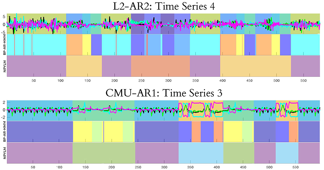
Figure 3. Plot of the first four dimensions of the input data and an example of segmentation results for both EB and UB steps. (Top) Toy data. (Bottom) CMU motion data.

Confusion matrices for the EB labels (left) and UB labels (right) of an example segmentation results are also illustrated in Figure 4. Here, the correspondence between true labels and estimated labels is represented with the values normalized per column, to allow one-to-many correspondence from a true label to estimated labels. Columns with entries close to 1 indicate that corresponding estimated labels are assigned with high specificity, while rows with multiple entries close to 1 indicate multiple estimated labels correspond to one true label.

FIGURE 4

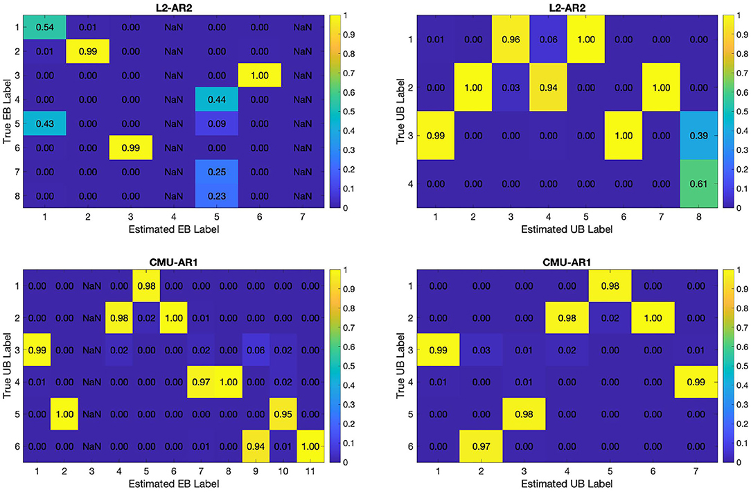
Figure 4. Confusion matrices for an example of segmentation results for both EB and UB steps. Numbers normalized per column. (Top) Toy data. (Bottom) CMU motion data.

Next, we evaluated the effects of model mismatch to segmentation, using the resulting average normalized Hamming distances between the true EBs and the estimated EBs (EB HDist). Hamming distances were computed as the total number of time steps where the estimated label was different from the ground truth in a given sequence, then summed for all time series sequences in each run. Then, normalization was done by dividing the Hamming distance by the total number of time steps of the given sequence The EB HDist were smallest when the true AR order was used. For example, EB HDist of L1-AR1 were smaller than those of L1-AR2 and L1-AR3, as seen in Figure 5. Similar results were observed in the cases of Sets L2 and L3. Note that this tendency was also observed in their respective adjusted Rand index (ARI) (right figures in Figure 5) and joint log probabilities of data and sample variables (Figure 6). The joint log probability P(y, F, z) is available even without the ground truth. Thus, the joint log probability can be a potential criterion for selecting the model with cross-validation.

FIGURE 5

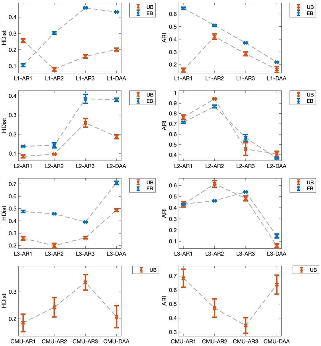
Figure 5. Evaluation of model accuracy. (Left) Average normalized Hamming distances. Bars: 1 SE. Lower value is better. (Right) Average adjusted Rand index. Bars: 1 SE. Higher value is better.

FIGURE 6

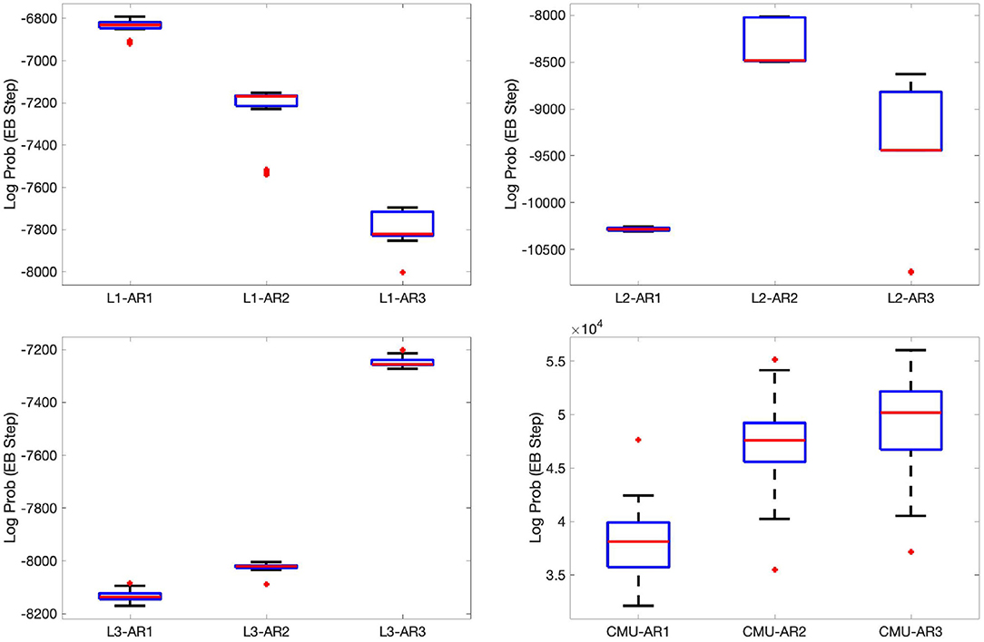
Figure 6. Boxplots of the joint log probabilities P(y, F, z) of the EB step. Red line: median. Edges of blue box: first and third quartiles. Whiskers: most extreme data points except outliers.

Finally, when we compared the normalized HDist of our method (selected using the joint log probabilities) with that of DAA, our method generally had better results than DAA. L2-AR2 and L3-AR3, which have the highest joint log probability among used models, have smaller EB HDist and UB HDist than L2-DAA and L3-DAA, respectively. In the case of L1, L1-AR1 shows smaller EB HDist than L1-DAA, but larger UB HDist. Even in this case, L1-AR2 shows better performance than L1-DAA. In summary, these results indicate the superiority of our method to DAA (Figure 5).

Aside from having better results compared to DAA, our method has other advantages. First, we note that the second step of our method reduces the error observed (left figures in Figure 5). Except for the results of L1-AR1, UB HDist are generally smaller than EB HDist. Even when segmentation in the EB level is wrong, correct segmentation in UB level is still possible, provided that the wrong pattern extraction of EB is reproduced for segments of same UBs. Second, it was also seen that the number of discovered EBs, including the EBs and the resulting segmentation, for each run varied (Figure 8). Despite this, the segmentation results at the UB step were more or less similar, as seen in the computed UB HDist. This observation indicates our method can identify the same UBs despite discovering different EBs. In other words, our method can absorb the difference of estimated EBs among different runs.

3.2.1. Large-Scale Toy Data

Results from subdataset Ts (s = 10, 20, 100) suggest that using our proposed method on larger datasets would yield more discovered EB labels (13.90, 17.70, 21.33) and formed UB labels (21.00, 19.70, 39.33). This then causes multiple discovered labels to correspond to the same ‘true' label. Adjusting for this when computing for EB and UB HDist, the computed EB HDist are 0.6112, 0.6759, and 0.7086 for T10, T20, and T100, respectively, while the corresponding UB HDist are 0.1096, 0.1633, and 0.1864, respectively. These results are consistent with our earlier observation that the second step of our method reduces observed errors in the first step. That is, correct segmentation in UB level is possible despite having errors in EB level segmentation, and regardless of the number of time series sequences considered.

4. Motion Data Experiments

Aside from synthetic experiments, motion data was also used in segmentation experiments. This is to see the applicability of proposed method to segment actual motion sequences.

4.1. Real Motion Data

To determine the effectiveness of our method with real motion data, one dataset was generated using the motion capture sequences of the actions of Subjects 18–23 in CMU Graphics Lab—Motion Capture Library (CMU, 2009). The dataset has four time series sequences of 16 dimensions that correspond to 8 joint angles of 2 individuals. The time series $\left\{{\text{y}}_t^{(i)}\right\}$ (i = 1, 2, 3, 4) were generated by concatenating UBs randomly chosen from six fixed types. The six UBs were the following actions: (1) walk toward each other than shake hands, (2) linked arms while walking, (3) synchronized walking, (4) alternating squats, (5) alternating jumping jacks, and (6) synchronized jumping jacks.

To evaluate the applicability of our method to real motion data, our method with AR orders (r = 1, 2, 3) was applied to the dataset. The parameters in our method were set in the same way as the previous section 3.1, but with κ = 200. Similar to toy data, our method was also compared with DAA using CMU dataset. State sequences were processed similar to the toy data, but with no states being discarded, as the states switched frequently in the first step of DAA.

4.2. Real Motion Data Applicability

Similar to the experiments in the previous section, the result of our method with AR(r) applied to the CMU dataset was denoted by CMU-ARr, while CMU-DAA was used to denote results from DAA. In terms of the average normalized UB HDist, CMU-AR1 had the smallest error when compared with CMU-AR2 and CMU-AR3 (Figure 5). However, CMU-AR2 and CMU-AR3 had higher log probability than CMU-AR1 (Figure 5). The optimal AR order could not be determined from the joint log probabilities in this case. Another criterion is needed to choose an optimal AR order. There is no existing available criterion, because our method is a highly complex singular model.

Comparing with the results of DAA, our method again had better performance than DAA. CMU-AR1 had smaller UB HDist (0.1815) compared to CMU-DAA (0.2080) (Figure 5). Similarly, CMU-AR1 had higher UB ARI (0.6847) compared to CMU-DAA (0.6384) (Figure 5). Unlike the obtained results from our proposed method, DAA had more UBs and switches, due to oversegmentation (Figure 7).

FIGURE 7

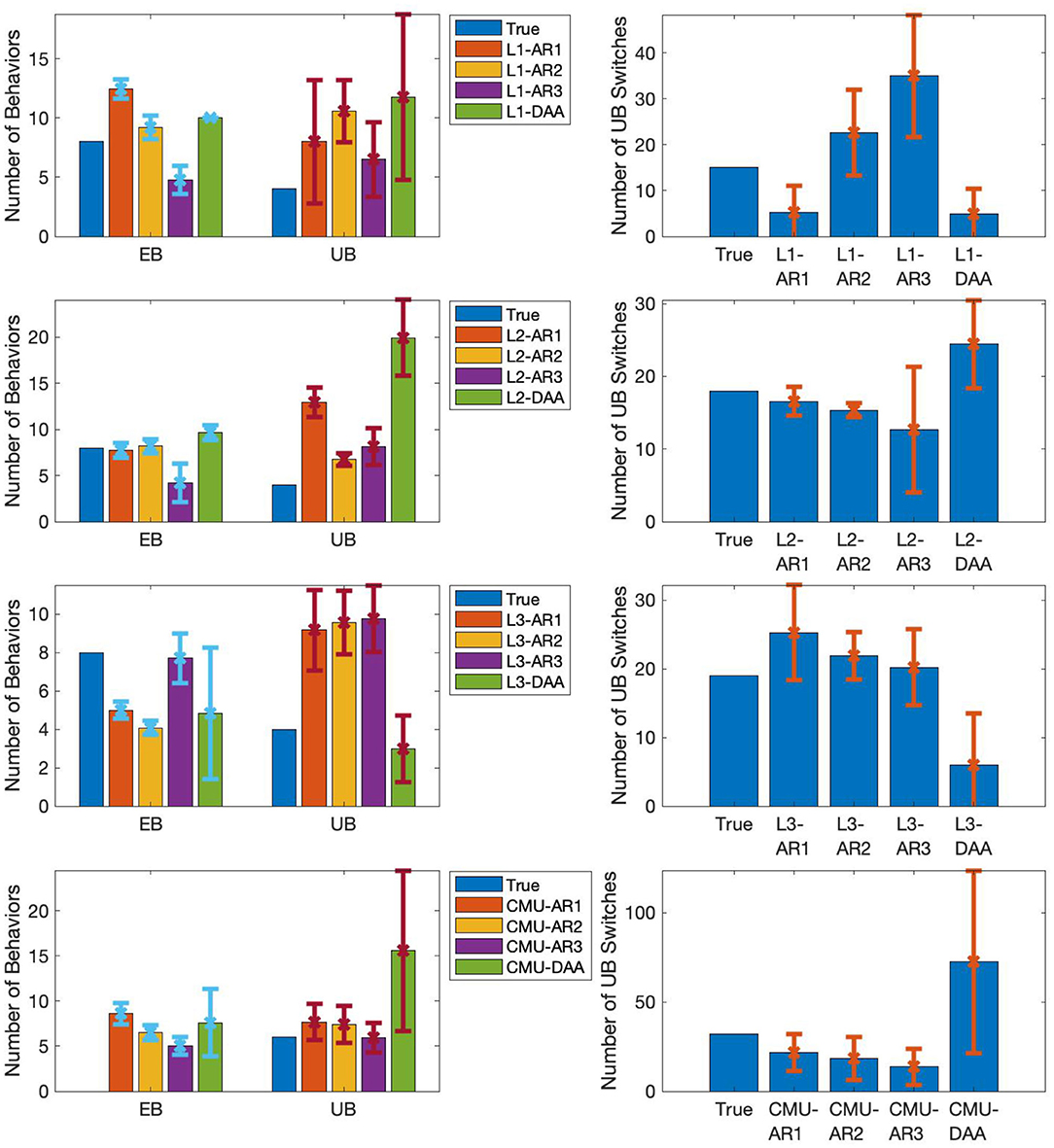
Figure 7. Switching characteristics of estimated labels. (Left) Average number of discovered EBs and UBs for each experiment. Bars: 1 SD. (Right) Average number of switches in all time series sequences for each experiment. Bars: 1 SD.

Finally, similar to the toy dataset results, the number of discovered EBs and the EB labels still varied for each run. However, the segmentation results of the UB step were quite similar (for example, see Figure 8). Here, the UB [1 8 1] refers to the alternating jumping jacks motion. In another segmentation, the same UB label corresponds to [D E], with the component EBs referring to completely different behaviors. Despite the difference in component EBs, both [1 8 1] and [D E] refer to the same true UB. Our method can thus identify the same semantic behaviors even from real motion data.

FIGURE 8

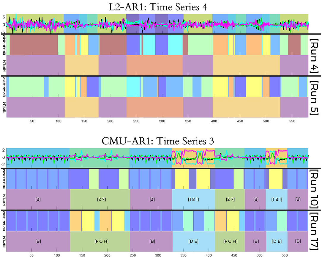
Figure 8. Plot of the first four dimensions of the input data and example segmentation results using our proposed method, obtained from two different runs. (Top) Toy data, with result from L2-AR1. (Bottom) CMU motion data, with result from CMU-AR1.

5. Discussion

To discover complex temporal patterns from the time series data via segmentation, we proposed a hierarchical non-parametric Bayesian approach. We combined the BP-AR-HMM and the double articulation by NPYLM to segment time series sequences under the assumption that they are generated from hierarchically-structured dynamical systems. In our results, we found that our method has better accuracy to discover temporal patterns than DAA for both the toy and real motion datasets. It may mean the necessity of dynamics to model local temporal patterns in time series data. Also, double articulation structure of our method would be suitable to extract semantic unit behaviors from unsegmented human motion sequences similar to DAA. In addition, our proposed method has another advantageous property over DAA. Our proposed method allows for asynchronous switching of segments, unlike DAA. It should be beneficial to extract temporal patterns from natural observation without any intervention, since we cannot expect consistent switching of behaviors under the natural observation. Despite these benefits, it should be noted that our proposed method is limited by its computational complexity. Furthermore, should the assumption of the sequence having a hierarchical structure not be met, our proposed method could not necessarily be appropriate to use.

Future directions are as follows: (1) using the estimated AR coefficients for interaction analysis and causality analysis, (2) a semi-supervised extension of the proposed method, and (3) automatic determination of AR order. Some methods of the causality analysis, e.g., Granger causality, are based on the AR models in their mathematical formulations. Therefore, we can use the estimated AR coefficient matrix to connect our method to causality analysis. With this combined approach, it will be possible to analyze switching causality. Next, it is usually difficult to have categorical labels for the entire dataset, but partial labels are easier to have. In this case, using semi-supervised segmentation could help improve the interpretability of results since some of the discovered components or states would correspond to the known categories. These labeled instances may also improve the identification of distribution of corresponding categories. A semi-supervised extension of our approach would thus be more effective to discover behavioral patterns. Finally, although we tried multiple settings of the AR order to select a model, automatic determination of AR order will solve this model selection problem.

We then conclude that our method can extract temporal patterns from multiple time series sequences by segmenting these sequences into low-level and high-level segments. Our method showed superior performance to a method called double articulation analyzer. Moreover, even when it discovered different low-level segments, our method can absorb such variation, and properly and consistently identify high-level segments.

Data Availability Statement

The datasets analyzed for this study can be found in the CMU Graphics Lab-Motion Capture Library (CMU, 2009).

Author Contributions

JB, TK, and KI contributed to the design and implementation of the research, to the analysis of the results, and to the writing of the manuscript. All authors contributed to the article and approved the submitted version.

Funding

This work was partially supported by JSPS KAKENHI 17H05863, 25118009, 15K16395, 17H05979, 16H06569, and 18K18108.

Conflict of Interest

The authors declare that the research was conducted in the absence of any commercial or financial relationships that could be construed as a potential conflict of interest.

References

Alazrai, R., Mowafi, Y., and Lee, C. S. G. (2015). Anatomical-plane-based representation for human-human interactions analysis. Pattern Recogn. 48, 2346–2363. doi: 10.1016/j.patcog.2015.03.002

PubMed Abstract | CrossRef Full Text | Google Scholar

Barbič, J., Safonova, A., Pan, J.-Y., Faloutsos, C., Hodgins, J., and Pollard, N. (2004). “Segmenting motion capture data into distinct behaviors,” in Proceedings of Graphics Interface (London, ON), 185–194.

Google Scholar

Briones, J., Kubo, T., and Ikeda, K. (2018). “A segmentation approach for interaction analysis using non-parametric Bayesian methods,” in Proceedings of the 62nd Annual Conference of the Institute of Systems, Control and Information Engineers (ISCIE) (Kyoto).

Google Scholar

Bruno, B., Mastrogiovanni, F., Sgorbissa, A., Vernazza, T., and Zaccaria, R. (2012). “Human motion modelling and recognition: a computational approach,” in 2012 IEEE International Conference on Automation Science and Engineering (CASE) (Seoul), 156–161. doi: 10.1109/CoASE.2012.6386410

CrossRef Full Text | Google Scholar

CMU (2009). Carnegie Mellon University Graphics Lab–Motion Capture Library. Available online at: http://mocap.cs.cmu.edu/

Fine, S., Singer, Y., and Tishby, N. (1998). The hierarchical hidden markov model: analysis and applications. Mach Learn. 32, 41–62. doi: 10.1023/A:1007469218079

CrossRef Full Text | Google Scholar

Fox, E., Sudderth, E., Jordan, M., and andWillsky, A. (2009). “Sharing features among dynamical systems with beta processes,” in Advances in Neural Information Processing Systems, Vol. 22, eds Y. Bengio, D. Schuurmans, J. D. Lafferty, C. K. I. Williams, and A. Culotta (Vancouver, BC: Curran Associates, Inc), 549–557.

Google Scholar

Fox, E., Sudderth, E., Jordan, M., and Willsky, A. (2008a). “An HDP-HMM for systems with state persistence,” in Proceedings of the 25th International Conference on Machine Learning (Helsinki), 312–319. doi: 10.1145/1390156.1390196

CrossRef Full Text | Google Scholar

Fox, E., Sudderth, E., Jordan, M., and Willsky, A. (2008b). “Nonparametric bayesian learning of switching linear dynamical systems,” in Advances in Neural Information Processing Systems, Vol. 21, eds D. Koller, D. Schuurmans, Y. Bengio, and L. Bottou (Vancouver, BC: Curran Associates, Inc), 457–464.

Google Scholar

Fox, E., Sudderth, E., Jordan, M., and Willsky, A. (2014). Joint modeling of multiple time series via the beta process with application to motion capture segmentation. Ann. Appl. Stat. 8, 1281–1313. doi: 10.1214/14-AOAS742

CrossRef Full Text | Google Scholar

Gilson, M., Tauste Campo, A., Thiele, A., and Deco, G. (2017). Nonparametric test for connectivity detection in multivariate autoregressive networks and application to multiunit activity data. Netw. Neurosci. 1, 357–380. doi: 10.1162/NETN_a_00019

PubMed Abstract | CrossRef Full Text | Google Scholar

Grigore, E. C., and Scassellati, B. (2017). “Discovering action primitive granularity from human motion for human-robot collaboration,” in Proceedings of Robotics: Science and Systems (Cambridge, MA).

Google Scholar

Harrison, L., Penny, W., and Friston, K. (2003). Multivariate autoregressive modeling of fMRI time series. Neuroimage 19, 1477–1491. doi: 10.1016/S1053-8119(03)00160-5

PubMed Abstract | CrossRef Full Text | Google Scholar

Heller, K., Teh, Y.W., and Gorur, D. (2009). “Infinite hierarchical hidden Markov models,” in Artificial Intelligence and Statistics, eds D. van Dyk and M. Welling (Clearwater, FL: PMLR), 224–231.

Google Scholar

Hughes, M. (2016). NPBayesHMM: Nonparametric Bayesian HMM Toolbox, for Matlab. Available online at: https://github.com/michaelchughes/NPBayesHMM

Hughes, M., Fox, E., and Sudderth, E. (2012). “Effective split-merge Monte Carlo methods for nonparametric models of sequential data,” in Advances in Neural Information Processing Systems, Vol. 25, eds F. Pereira, C. J. C. Burges, L. Bottou, and K. Q. Weinberger (Lake Tahoe, CA: Curran Associates, Inc), 1–9.

Google Scholar

Keogh, E., Chu, S., Hart, D., and Pazzani, M. (2004). “Segmenting time series: a survey and novel approach,” in Data Mining in Time Series Databases, eds M. Last, A. Kandel, and H. Bunke (World Scientific), 1–21. doi: 10.1142/9789812565402_0001

CrossRef Full Text | Google Scholar

Mochihashi, D., Yamada, T., and Ueda, N. (2009). “Bayesian unsupervised word segmentation with nested Pitman-Yor language modeling,” in Proceedings of the Joint Conference of the 47th Annual Meeting of the ACL and the 4th International Joint Conference on Natural Language Processing of the AFNLP: Volume 1–ACL-IJCNLP '09 (Singapore), Vol. 1, 100–108. doi: 10.3115/1687878.1687894

CrossRef Full Text | Google Scholar

Neubig, G. (2016). latticelm. Available online at: https://github.com/neubig/latticelm

Neubig, G., Mimura, M., Mori, S., and Kawahara, T. (2010). “Learning a language model from continuous speech,” in 11th Annual Conference of the International Speech Communication Association (InterSpeech 2010) (Makuhari), 1053–1056.

Google Scholar

Ryoo, M., and Aggarwal, J. (2009). Semantic representation and recognition of continued and recursive human activities. Int. J. Comput. Vis. 82, 1–24. doi: 10.1007/s11263-008-0181-1

CrossRef Full Text | Google Scholar

Saeedi, A., Hoffman, M., Johnson, M., and Adams, R. (2016). “The segmented iHMM: a simple, efficient hierarchical infinite HMM,” in International Conference on Machine Learning (New York, NY), 2682–2691.

Google Scholar

Taniguchi, T., and Nagasaka, S. (2011). “Double articulation analyzer for unsegmented human motion using Pitman-Yor language model and infinite hidden Markov model,” in 2011 IEEE/SICE International Symposium on System Integration, SII 2011 (Kyoto), 250–255. doi: 10.1109/SII.2011.6147455

CrossRef Full Text | Google Scholar

Taniguchi, T., Nagasaka, S., and Nakashima, R. (2016). Nonparametric Bayesian double articulation analyzer for direct language acquisition from continuous speech signals. IEEE Trans. Cogn. Dev. Syst. 8, 171–185. doi: 10.1109/TCDS.2016.2550591

CrossRef Full Text | Google Scholar

Viviani, P., and Cenzato, M. (1985). Segmentation and coupling in complex movements. J. Exp. Psychol. Hum. Percept. Perform. 11:828. doi: 10.1037/0096-1523.11.6.828

PubMed Abstract | CrossRef Full Text | Google Scholar

Williams, B., Toussaint, M., and Storkey, A. (2007). “Modelling motion primitives and their timing in biologically executed movements,” in Advances in Neural Information Processing Systems, Vol. 20, eds J. C. Platt, D. Koller, Y. Singer, and S. T. Roweis (Vancouver, BC: Curran Associates, Inc), 1609–1616.

Google Scholar

Zeger, S., Irizarry, R., and Peng, R. (2006). On time series analysis of public health and biomedical data. Annu. Rev. Public Health 27, 57–79. doi: 10.1146/annurev.publhealth.26.021304.144517

PubMed Abstract | CrossRef Full Text | Google Scholar

Zhou, F., Torre, F. D. L., and Hodgins, J. K. (2013). Hierarchical aligned cluster analysis for temporal clustering of human motion. IEEE Trans. Pattern Anal. Mach. Intell. 35, 582–596. doi: 10.1109/TPAMI.2012.137

PubMed Abstract | CrossRef Full Text | Google Scholar