 Alexander Krull
 Tomáš Vičar
 Mangal Prakash
 Manan Lalit
 Florian Jug
- 1Center for Systems Biology Dresden, Dresden, Germany
- 2Max Planck Institute for Molecular Cell Biology and Genetics, Dresden, Germany
- 3Max Planck Institute for Physics of Complex Systems, Dresden, Germany
- 4Department of Biomedical Engineering, Faculty of Electrical Engineering and Communication, Brno University of Technology, Brno, Czechia
Today, Convolutional Neural Networks (CNNs) are the leading method for image denoising. They are traditionally trained on pairs of images, which are often hard to obtain for practical applications. This motivates self-supervised training methods, such as Noise2Void (N2V) that operate on single noisy images. Self-supervised methods are, unfortunately, not competitive with models trained on image pairs. Here, we present Probabilistic Noise2Void (PN2V), a method to train CNNs to predict per-pixel intensity distributions. Combining these with a suitable description of the noise, we obtain a complete probabilistic model for the noisy observations and true signal in every pixel. We evaluate PN2V on publicly available microscopy datasets, under a broad range of noise regimes, and achieve competitive results with respect to supervised state-of-the-art methods.
1. Introduction
Image restoration is the problem of reconstructing an image from a corrupted version of itself. Recent work shows how CNNs can be used to build powerful content-aware image restoration (CARE) pipelines (Weigert et al., 2017, 2018; Zhang et al., 2017, 2019; Lehtinen et al., 2018; Batson and Royer, 2019; Krull et al., 2019; Laine et al., 2019). However, for traditional supervised CARE models (Weigert et al., 2018) pairs of clean and noisy images are required.
For many application areas, it is impractical or impossible to acquire clean ground-truth images. In such cases, Noise2Noise (N2N) training (Lehtinen et al., 2018) relaxes the problem, only requiring two noisy instances of the same data. Unfortunately, even the acquisition of two noisy realizations of the same image content is often difficult (Buchholz et al., 2019). Self-supervised training methods, such as Noise2Void (N2V) (Krull et al., 2019), are a promising alternative, as they operate exclusively on single noisy images (Batson and Royer, 2019; Krull et al., 2019; Laine et al., 2019). This is enabled by excluding/masking the center (blind-spot) of the network's receptive fields. Self-supervised training assumes that the noise is pixel-wise independent and that the true intensity of a pixel can be predicted from local image context, excluding before-mentioned blind-spots (Krull et al., 2019). For many applications, especially in the context of microscopy images, the first assumption is fulfilled, but the second assumption offers room for improvements (Laine et al., 2019).
Hence, self-supervised models can often not compete with supervised training (Krull et al., 2019). In concurrent work (Laine et al., 2019) this problem was elegantly addressed by assuming a Gaussian noise model and predicting Gaussian intensity distributions per pixel. The authors also showed that the same approach can be applied to other noise distributions, which can be approximated as Gaussian, or can be described analytically.
Here, we introduce a new training approach called Probabilistic Noise2Void (PN2V). Similar to Laine et al. (2019), PN2V proposes a way to leverage information of the network's blind-spots. However, PN2V is not restricted to Gaussian noise models or Gaussian intensity predictions. More precisely, to compute the posterior distribution of a pixel, we combine (i) a general noise model that can be represented as a histogram (observation likelihood), and (ii) a distribution of possible true pixel intensities (prior), represented by a set of predicted samples.
Having this complete probabilistic model for each pixel, we are now free to chose which statistical estimator to employ. In this work we use minimum mean square error (MMSE) estimates for our final predictions. Alternatively to using MMSE, one could use other estimates, such as the mean absolute error (MAE), the maximum a posteriori estimation (MAP), or a Huber loss (smooth MAE). The reason to choose the MMSE is motivated by our desire to minimize the PSNR of our predictions with respect to the ground-truth data. In this work we show that MMSE-PN2V consistently outperforms other self-supervised methods, and in many cases, leads to results that are competitive even with supervised state-of-the-art CARE networks.
2. Related Work
Denoising algorithms that do not require paired training have existed for a number of years. Here, we will give a brief overview of such methods, discussing their strengths and limitations.
2.1. Classical Filtering Methods
Many classical denoising techniques are based on the idea of “intelligent” averaging. That is, they compute the estimate for each pixel as a weighted average of other pixels in the image. All these techniques do not require training data of any kind. Today, all such training-free methods are outperformed by learning based systems.
The bilateral filter (Tomasi and Manduchi, 1998) calculates every pixel's output by averaging a local neighborhood. It uses each pixels's distance in image and color space to determine its influence.
The non-local means algorithm, introduced by Buades et al. (2005), goes one step further. Building on the self similarity of natural images, they calculate each pixel's estimate as an average of multiple pixels that can be located anywhere in the image. Pixel weights are based on the similarity of surrounding image patches.
An improved variation of the same idea was introduced by Dabov et al. (2007) under the name block-matching and 3D filtering (BM3D). Dabov et al. identify similar patches of the image and group them in a 3D volume, on which filtering is applied. These filtered patches are then projected back into the original image.
Like our PN2V, the above methods can be interpreted from a probabilistic point of view. Milanfar (2012) provides a in-depth discussion of this perspective. He shows that the calculation of pixel weights, can indeed be seen as the ad-hoc construction of a local image prior. This is similar to PN2V, which uses a blind-spot network to predict a prior distribution for each pixel. A major difference is that PN2V can learn these priors beforehand from training data, while the classical averaging methods can only exploit self similarities in the current image to be denoised in order to compute this prior.
2.2. Stein's Unbiased Risk Estimator
Stein (1981) published a seminal paper on estimating the mean of normal distributed random variables–an equivalent task to the removal of additive Gaussian noise. The risk of such an estimator, given be expected quadratic error, can be computed from the noisy realizations alone without requiring clean examples. His formulation is based on the derivative of the estimate with respect to the input. This method is known as Stein's unbiased risk estimator (SURE).
Ramani et al. (2008) showed that SURE can be used to tune the parameters of a variety of denoising algorithms, based on noisy images alone. Since SURE requires the calculation of the estimator's derivatives, Ramani et al. introduce an efficient Monte Carlo approximation that allows for an application with algorithms that are not easily differentiable.
Only very recently, Metzler et al. (2018) as well as Soltanayev and Chun (2018) applied this approach for the training of denoising CNNs and use SURE (including the Monte Carlo approximation) as loss function. This allows them to train a network for the removal of Gaussian noise based purely on noisy training data.
Like PN2V, SURE based methods require knowledge of the noise model (the standard deviation of Gaussian noise) to allow training from individual noisy images. While extensions of SURE for specific non-Gaussian noise models have been proposed (Raphan and Simoncelli, 2007; Luisier et al., 2010) they have not been utilized for the training of neural networks. PN2V, on the other hand, is designed to incorporate general and empirically measured noise models. Even though (P)N2V and SURE attack the training problem from orthogonal angles, their respective loss functions show a curious resemblance. We believe that there is a deeper theoretical connection, worth to be explored in future work.
2.3. Deep Image Prior
The work by Ulyanov et al. (2018) is yet another interesting approach to be mentioned. The authors discovered that the structure of CNNs “resonates” with natural images and is inherently suitable for the task of denoising and image restoration. Ulyanov et al. train a network to predict a single noisy image from a constant random input. Similarly to (P)N2V, they use the noisy data itself as target. They find that when the training process is stopped at a suitable time, the network can produce a noise free version of the given image.
The downside of this approach is that a separate network has to be trained for each image to be denoised. Additionally, the correct moment to stop the training is not easily predicable. In contrast, PN2V has to be trained only once and, provided enough data is available, until convergence.
3. Background
3.1. Image Formation and the Denoising Task
An image x = (x1, …, xn) is the corrupted version of a clean image (signal) s = (s1, …, sn). Our goal is to recover the original signal from x, thus implementing a function .
In this paper, we assume that each observed pixel value xi is independently drawn from the conditional distribution p(xi|si) such that
We will refer to p(xi|si) as observation likelihood. It is described by an arbitrary noise model. As we will see later, this noise model can usually be computed from a simple stack of calibration images. It does not depend on the content of the images that are to be denoised.
3.2. Traditional Training and Noise2Noise
The function f(x) can be implemented by a Fully Convolutional Network (FCN) (Long et al., 2015) (see e.g., Weigert et al., 2017, 2018; Zhang et al., 2017; Lehtinen et al., 2018), a type of CNN that takes an image as input and produces an entire (in this case denoised) image as output. However, in this setup every predicted output pixel depends only on a limited receptive field xRF(i), i.e., a patch of input pixels surrounding it. FCN based image denoising in fact implements f(x) by producing independent predictions for each pixel i, depending only on xRF(i) instead of on the entire image. The prediction is parameterized by the weights θ of the network.
In traditional training, θ are learned from pairs of noisy xj and corresponding clean training images sj, which provide training examples consisting of noisy input patches and their corresponding clean target values . The parameters θ are traditionally tuned to minimize an empirical risk function, such as the mean squared error (MSE)
over all training images j and pixels i.
In Noise2Noise, Lehtinen et al. (2018) show that clean data is in fact not necessary for training and that the same training scheme can be used with noisy data alone. Noise2Noise uses pairs of corresponding noisy training images xj and x′j, which are based on the same signal sj, but are corrupted independently by noise (see Equation 1). Such pairs can, for example, be acquired by imaging a static sample twice. Noise2Noise uses training examples , with the input patch cropped from the first image xj and the noisy target extracted from the patch center in the second image x′. It is not possible for the network to predict the noisy pixel value from the independently corrupted input . However, assuming the noise is zero centered, i.e., the best achievable prediction is the clean signal and the network will learn to denoise the images it is presented with.
3.3. Noise2Void Training
In Noise2Void (Krull et al., 2019), the authors show that training is still possible when not even noisy training pairs are available. They use single images to extract input and target for their networks. If this was done naively, the network would simply learn the identity, directly outputting the value at the center of each pixel's receptive field. Krull et al. address the issue by effectively removing the central pixel from the network's receptive field. To achieve this, they mask the pixel during training, replacing it with a random value from the vicinity. Thus, a Noise2Void trained network can be seen as a function making a prediction for a single pixel based on the modified patch that excludes the central pixel. Such a network can no longer describe the identity and can be trained from single noisy images.
However, this ability comes at a price. The accuracy of the predictions is reduced, as the network has to exclude the central pixel of its receptive field, thus having less information available for the prediction at hand.
To allow efficient training of a CNN with Noise2Void, Krull et al. simultaneously mask multiple pixels in larger training patches and jointly calculate their gradients.
4. Methods
4.1. Maximum Likelihood Training
In PN2V, we build on the idea of masking pixels (Krull et al., 2019) to obtain a prediction from the modified receptive field . However, instead of directly predicting an estimate for each pixel value, PN2V trains a CNN to describe a probability distribution
We will refer to as prior, as it describes our knowledge of the pixel's signal considering only its surroundings, but not the observation at the pixel itself xi, since it has been excluded from . We choose a sample based representation for this prior, which will be discussed below.
Remembering that the observed pixels values are drawn independently (Equation 1), we can combine Equation (3) with our noise model, and obtain the joint distribution
By integrating over all possible clean signals, we can derive
the probability of observing the pixel value xi, given we know its surroundings . We can now view CNN training as an unsupervised learning task. Following the maximum likelihood approach, we tune θ to minimize
Note that in order to improve readability, from here on we will omit the index j and refrain from explicitly referring to the training image.
4.2. Sample Based Prior
To allow an efficient optimization of Equation (6) we choose a sample based representation of our prior . For every pixel i, our network directly predicts K = 800 output values , which we interpret as independent samples, drawn from . We can now approximate Equation (6) as
During training we use Equation (7) as loss function. Note that the summation over k can be efficiently performed on the GPU.
Since every sample is effectively a function of the parameters θ, we can calculate the derivative with respect to any network parameter θl as
It is important to note that our loss function naturally prevents a concentration of samples and encourages them to spread out to describe the prior distribution. To see why this is the case, let us consider a hypothetical situation in which all samples are tightly packed around some value c, that is,
Considering that the samples are predicted by a blind-spot network without knowledge of the observed value xi, it is likely that such a clustered configuration can sometimes lead to a low observation likelihood for all samples . In such a situation, the logarithm in Equation (7) will produce a potentially infinite loss. However as soon as one of the samples were to move away from the cluster in the right direction and produces a somewhat increased likelihood , the loss would immediately drop dramatically, leading to a strong gradient in this direction and an incentive to spread the samples.
4.3. Minimum Mean Squared Error Inference
Assuming our network is sufficiently trained, we are now interested in processing images and finding sensible estimates for every pixel's signal si. Based on our probabilistic model, we derive the MMSE estimate, which is defined as
where p(si|xRF(i)) is the posterior distribution of the signal given the complete surrounding patch. The posterior is proportional to the joint distribution given in Equation (4). We can thus approximate by weighing our predicted samples with the corresponding observation likelihood and calculating their average
Figure 1 illustrates the process and shows the involved distributions for a concrete pixel in a real example. Further illustrations for multiple pixels can be found in Supplementary Figures 1, 2.
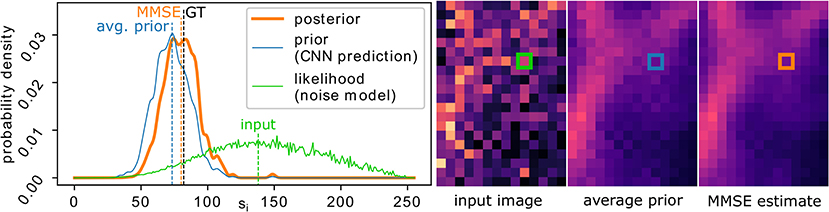
Figure 1. Image denoising with PN2V. The final MMSE estimate (orange dashed line) for the true signal si of a pixel (position marked in the image insets on the right) corresponds to the center of mass of the posterior distribution (orange curve). Given an observed noisy input value Xi (dashed green line), the posterior is proportional to the product of the prior (blue curve) and the observation likelihood (green curve). PN2V describes the prior by a set of samples predicted by our CNN. The likelihood is provided by an arbitrary but measured noise model. The black dashed line indicated the true signal of the pixel (GT). Prior and posterior are visualized using a kernel density estimator.
5. Experiments
The results of our main experiments can be found in Table 1. In Figure 2, we provide qualitative results on test images. Further qualitative results for different noise regimes can be found in Supplementary Figure 3. Supplementary Figures 4, 5 show the distribution of uncertainty in the predictions.
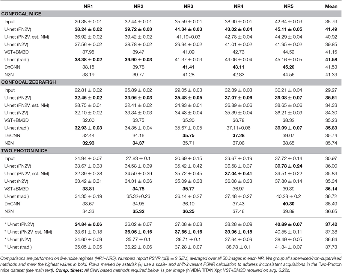
Table 1. Results of PN2V and baseline methods on three datasets from Zhang et al. (2019).
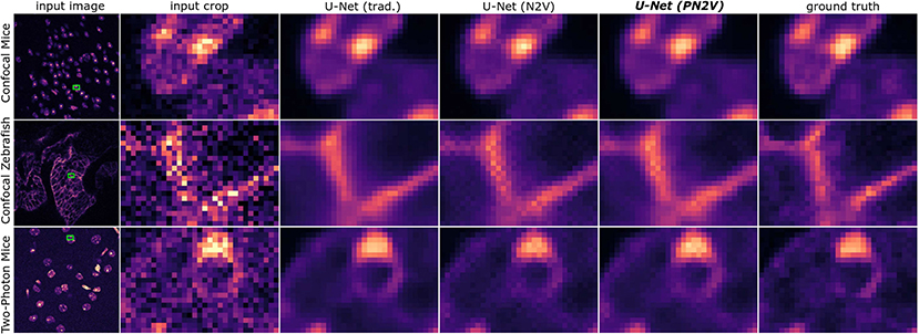
Figure 2. Qualitative results for three images (rows) from the datasets we used in this manuscript. Left to right: raw image (NR1), zoomed inset, predictions by U-Net (trad.), U-Net (N2V), U-Net (PN2V), and ground-truth data.
We discuss additional experiments on the importance of the noise model section 5.4.
5.1. Datasets
We evaluate PN2V on datasets provided by Zhang et al. (2019). Since PN2V is not yet implemented for multi-channel images, we use all available single-channel datasets.
These datasets are recorded with different samples and under different imaging conditions. Each of them consists of a total of 20 fields of view (FOVs). One FOV is reserved for testing. The other 19 are used for training and validation.
For each FOV, the data is composed of 50 raw microscopy images, each containing different noise realizations of the same static sample. For every FOV, Zhang et al. (2019) additionally simulate 4 reduced noise regimes (NRs) by averaging different subsets of 2, 4, 8, and 16 raw images. We will refer to the raw images as NR1 and to the regimes created through averaging 2, 4, 8, and 16 images as NR2, NR3, NR4, and NR5, respectively. The ground-truth is created by averaging all 50 raw images. This kind of ground-truth data fits particularly well for methods like N2N, N2V, or PN2V, where it is assumed that the clean signal corresponds to the expected value of independent noise realizations (section 3.2) and is not arbitrarily shifted or scaled, as is the case in other datasets, such as Weigert et al. (2018).
We find that in one of the datasets (Two-Photon Mice) the average pixel intensity fluctuates heavily over the course of the 50 images, even though it should be approximately constant for each FOV. Considering that a single ground-truth image (the average) is used for the evaluation on all 50 images, this leads to fluctuations and distortions in the calculated peak signal to noise ratios (PSNRs), which are also reflected in the comparatively high standard errors (SEMs) for all methods (see Table 1). To account for this inconsistency in the data, we additionally use a variant of the PSNR calculation that is invariant to arbitrary shifts and linear transformations in the ground-truth signal (Weigert et al., 2018). These values are marked by an asterisk.
5.2. Noise Models
In our experiments, we use a histogram based method to measure and describe the noise distribution p(xi|si). We start with corresponding pairs of clean sj and noisy xj images. For this purpose, we use the available training data from Zhang et al. (2019). However, these images could show an arbitrary pattern, covering the desired range of values and do not have to resemble the sample we are interested in. This process is illustrated in Figure 3. We construct a 2D histogram (256 × 256 bins), with the y- and x-axis corresponding to the clean and noisy pixel values , respectively. By normalizing every row, we obtain a probability distribution for every signal. Considering Equation (7), we require our model to be differentiable with respect to the si. To ensure this differentiability, we linearly interpolate along the y-axis of the normalized histogram, obtaining a model for p(xi|si) that is continuous in si.
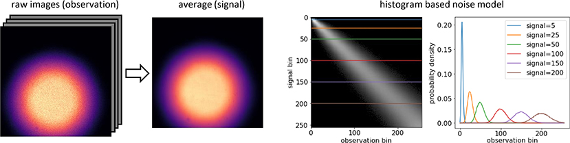
Figure 3. Recording a histogram based noise model for a particular microscope. (Left) A noise model can be calculated from a stack of calibration images, showing any fixed content that covers the range of signals we are interested in. Noise models capture the noise property of the camera and are sample independent. In most microscopes, one can collect a calibration sequence without even having a sample to image. The example shows an out-of-focus, halfway closed field diaphragm. The only purpose of these images is to create data that contains a non-saturated range of image intensities that cover the desired signal domain. Here we collect a set of 100 noisy raw images (observations). Provided that nothing in our setup moved, we can estimate the corresponding true signal by averaging. (Right) Using the pairs of clean signal and noisy observations we can now produce a 2D histogram (see section 5.2), with each row corresponding to the distribution p(xi|si) for a particular signal si. The plot shows these distributions for six different signal values, as indicated by color.
5.3. Evaluated Denoising Models/Methods
To put the denoising results of PN2V into perspective, we compare to various state-of-the-art baselines, including the strongest published numbers on the used datasets. We compare the following methods:
U-Net (PN2V): We use a standard U-Net (Ronneberger et al., 2015)1. Our network has a U-Net depth of 3, one input channel, and K = 800 output channels, which are interpreted as samples. We start with an initial feature channel number of 64 in the first U-Net layer. To train our blind-spot network we use the same masking technique (UPS with window size of 5 × 5) as Krull et al. (2019), simultaneously masking 312 pixels in every training patch. We train our network separately for each NR in each dataset, each time reserving the last five training images as validation set. For optimization we use the Adam optimizer (Kingma and Ba, 2014) with an initial learning rate of 10−4 and standard parameters. The learning rate is reduced when the validation loss hits a plateau2. Training continues over 200 epochs, each consisting of 50 steps. In each step we process a batch of 80 training patches. Training patches are 100 × 100 pixels in size and are randomly cropped and augmented by random (90, 180, 270°) rotations and flipping.
U-Net (PN2V, est. NM): We use the same network architecture and settings as for U-Net (PN2V). However, instead of using the noise model as described in section 5.2, we estimate an approximate Poisson Gaussian noise model from each training image using the code from Foi et al. (2008). We average the resulting parameters for each dataset and noise regime and populate our noise model histogram with the respective values. We use this noise model during training and testing.
U-Net (N2V): We use the same network architecture as for U-Net (PN2V) but modify the output layer to produce only a single prediction instead of K = 800. The network is trained using the Noise2Void scheme as described by Krull et al. (2019). All training parameters are identical to U-Net (PN2V).
U-Net (trad.): We use the exact same architecture as U-Net (N2V), but train the network using the available ground-truth data and the standard MSE loss (see Equation 2). All training parameters are identical to U-Net (PN2V) and U-Net (N2V).
VST+BM3D: Numbers are taken from Zhang et al. (2019). The authors fit a Poisson Gaussian noise model to the data and then apply a combination of variance-stabilizing transformation (VST) (Makitalo and Foi, 2013) and BM3D filtering (Dabov et al., 2007).
DnCNN: Numbers are taken from Zhang et al. (2019). DnCNN (Zhang et al., 2017) is an established CNN based denoising architecture that is trained in a supervised fashion.
N2N: Numbers are taken from Zhang et al. (2019). The authors train a network according to the N2N scheme, using an architecture similar to the one presented in Lehtinen et al. (2018).
5.4. Importance of a Good Noise Model
In this section we want to (i) demonstrate how a suitable noise model can be recorded for a given microscope and (ii) investigate the effect of sub-optimal noise models. To this end, we acquired calibration dataset and images to be denoised on a spinning disk confocal microscope3.
A noise model can be calculated from a stack of calibration images. The structural content of these images is irrelevant, as long as all desired signal intensities are well-covered. In most microscopes, one can, e.g., collect such a calibration sequence by simply acquiring images of the halfway closed, out-of-focus field diaphragm (see Figure 3). Hence, we collected 100 noisy images of this static scene and estimated the corresponding true signal by averaging. In order to derive a complete noise model, we collected histograms of noisy pixel realizations for each true signal intensity in the ground-truth image.
Next, we needed to image a fluorescent sample for denoising. Here we chose a fixed Convallaria cross section that was readily available in our light microscopy facility. Again, we acquired 100 noisy images (1,024 × 1,024 pixels) of the same field of view of the same sample. This allowed us, as in Zhang et al. (2019), to average all 100 images and create an approximately noise free pseudo ground-truth. Finally, we subdivided the data into four equally sized quadrants. PN2V models were trained on data of all four quadrants, but the traditionally trained baseline (which needs clean ground-truth images during training) was only trained on three quadrants, leaving one quadrant for testing.
In order to create a series of noise models of decreasing quality, we computed those as described above, but artificially reduced the amount of available calibration data. More specifically, we sub-sampled the raw calibration data, initially using 10% of the pixels, then 1%, and in the most extreme case only 1 in 100,000 pixels.
Finally, we used this sequence of noise models to train the respective PN2V networks and predict their corresponding denoised MMSE images. In Figures 4, 5, we show these results. Note that all trained networks use the same architectures we described in earlier sections, with the only difference that we have increased the learning rate to 10−3, performed only five training steps per epoch, and used an effective batch size of 20.
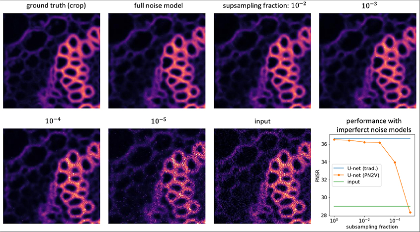
Figure 4. Importance of good noise models. Images show a representative crop of the Convallaria data we describe in the main text. From top left to bottom right we show the ground-truth, a PN2V prediction using all available calibration data, four PN2V results on increasingly sub-sampled calibration data (see main text for details), and the corresponding noisy input crop. The plot shows the quality of PN2V denoising (PSNR) on full and increasingly sub-sampled noise models (orange), the PSNR of a traditionally trained U-Net (blue), and the PSNR of the noisy input (green). Interestingly, When a noise model is derived from too little calibration data, PSNR values decrease dramatically, even below the quality of the noisy input data. Still, for sufficiently large fractions, PN2V almost reaches the performance of traditional supervised training, despite never having seen a single ground-truth pixel.
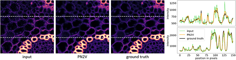
Figure 5. Edge preservation in PN2V reconstructions. Here we show that the content-awareness of PN2V makes it perfectly capable of restoring sharp image gradients (edges). From left to right, we show an Convallaria image patch and the corresponding PN2V restoration and ground-truth. The rightmost column shows line-plots along the dashed white lines in all three images.
While the experiments we described here show that noise models based on insufficient calibration data lead to lower quality PN2V predictions, they also show that 100 diaphragm images are sufficient to derive high quality noise models.
6. Discussion
We have introduced PN2V, a fully probabilistic approach extending self-supervised CARE training. PN2V makes use of an arbitrary noise model which can be determined by analyzing any set of available images that are subject to the same type of noise. This is a decisive advantage compared to state-of-the-art supervised methods and allows PN2V to be used for many practical applications.
The improved performance of PN2V lies consistently beyond other self-supervised methods and can often compete with state-of-the-art supervised methods, such as CARE (Weigert et al., 2018). In Figure 5 we show that the content-awareness of PN2V allows it to reconstruct sharp image gradients (edges), despite never being shown clean ground-truth data. We see a plethora of unique applications for PN2V, for example in low-light live-cell experiments, where noise typically is the limiting factor for downstream analysis.
Additionally, we find that an adequate noise model is of critical importance to achieve optimal results. Networks using blindly estimated noise models (PN2V, est. NM) are clearly outperformed by networks using the correct model. The only exception is the (Two-Photon Mice) dataset. Here, the estimated noise models appear to even outperform the supervised baseline. However, as mentioned before, this particular dataset is characterized by unstable illumination (see section 5.1), which affects training, as well as the ground-truth used for PSNR calculation.
In practice, we see the requirement for a high quality noise model only as a minor caveat: The model does not depend on the sample and has to be recorded only once, which seems to be an acceptable overhead, considering the improved denoising performance.
Data Availability Statement
The data used in our experiments is published by Zhang et al. (2019) and available at: http://tinyurl.com/y6mwqcjs. The PN2V source code is available at: https://github.com/juglab/pn2v.
Author Contributions
AK and TV jointly developed the theory in discussion with FJ. AK and FJ designed the experiments. AK implemented the software and ran all the experiments. AK and TV analyzed the results. MP and ML performed the additional experiments on the importance on the noise model. All authors contributed in writing the manuscript.
Funding
Funding was provided from the core budget of the Max Planck Institute for Molecular Cell Biology and Genetics, the Max Planck Institute for Physics of Complex Systems, and the Brno University of Technology, as well as, by the German Federal Ministry of Research and Education under the code 01IS18026C, ScaDS2).
Conflict of Interest
The authors declare that the research was conducted in the absence of any commercial or financial relationships that could be construed as a potential conflict of interest.
Acknowledgments
We thank Uwe Schmidt, Martin Weigert, and Tobias Pietzsch for the helpful discussions. We thank Tobias Pietzsch, Tim-Oliver Buchholz, and Dorit Kämpfer for proof reading. We also thank Peyman Milanfar for his series of informative tweets on the history of denoising. The computations were performed on an HPC Cluster at the Center for Information Services and High Performance Computing (ZIH) at TU Dresden. We thank the MPI-CBG Computer Department and Light Microscopy Facility (LMF) for their support. In particular we want to thank Britta Schroth-Diez for her assistance in recording the Convallaria dataset.
Supplementary Material
The Supplementary Material for this article can be found online at: https://www.frontiersin.org/articles/10.3389/fcomp.2020.00005/full#supplementary-material
Footnotes
1. ^We utilize the pytorch implementation from https://github.com/jaxony/unet-pytorch, setting the merge_mode parameter to “concat” and up_mode parameter to “transpose.”
2. ^We use the pytorch optim.lr_scheduler.ReduceLROnPlateau with a patience parameter of 10 and a reduction factor of 0.5.
3. ^We use an Andor Revolution WD Borealis Mosaic with an Andor iXon Ultra 888 Monochrome EMCCD camera and EM-gain 130.
References
Batson, J., and Royer, L. (2019). “Noise2self: blind denoising by self-supervision” in Proceedings of the 36th International Conference on Machine Learning ICML, Vol. 97 (Long Beach, CA).
Buades, A., Coll, B., and Morel, J.-M. (2005). “A non-local algorithm for image denoising,” in 2005 IEEE Computer Society Conference on Computer Vision and Pattern Recognition (CVPR'05), Vol. 2 (San Diego, CA: IEEE), 60–65.
Buchholz, T.-O., Jordan, M., Pigino, G., and Jug, F. (2019). “Cryo-care: content-aware image restoration for cryo-transmission electron microscopy data,” in IEEE 16th International Symposium on Biomedical Imaging (ISBI) (Venice).
Dabov, K., Foi, A., Katkovnik, V., and Egiazarian, K. (2007). Image denoising by sparse 3-D transform-domain collaborative filtering. IEEE Trans. Image Process. 16, 2080–2095. doi: 10.1109/TIP.2007.901238
Foi, A., Trimeche, M., Katkovnik, V., and Egiazarian, K. (2008). Practical Poissonian-Gaussian noise modeling and fitting for single-image raw-data. IEEE Trans. Image Process. 17, 1737–1754. doi: 10.1109/TIP.2008.2001399
Kingma, D. P., and Ba, J. (2014). Adam: a method for stochastic optimization. arXiv[Preprint]. arXiv:1412.6980.
Krull, A., Buchholz, T.-O., and Jug, F. (2019). “Noise2void–learning denoising from single noisy images,” in Conference on Computer Vision and Pattern Recognition (CVPR) (Long Beach, CA), 2129–2137.
Laine, S., Karras, T., Lehtinen, J., and Aila, T. (2019). “High-quality self-supervised deep image denoising” in Advances in Neural Information Processing Systems (NeurIPS) (Vancouver, BC), 6968–6978.
Lehtinen, J., Munkberg, J., Hasselgren, J., Laine, S., Karras, T., Aittala, M., et al. (2018). “Noise2Noise: learning image restoration without clean data,” in Proceedings of the 35th International Conference on Machine Learning (ICML), Vol. 80 (Stockholm), 2965–2974.
Long, J., Shelhamer, E., and Darrell, T. (2015). “Fully convolutional networks for semantic segmentation,” in CVPR (Boston, MA), 3431–3440.
Luisier, F., Blu, T., and Unser, M. (2010). Image denoising in mixed Poisson–Gaussian noise. IEEE Trans. Image Process. 20, 696–708. doi: 10.1109/TIP.2010.2073477
Makitalo, M., and Foi, A. (2013). Optimal inversion of the generalized anscombe transformation for poisson-gaussian noise. IEEE Trans. Image Process. 22, 91–103. doi: 10.1109/TIP.2012.2202675
Metzler, C. A., Mousavi, A., Heckel, R., and Baraniuk, R. G. (2018). Unsupervised learning with stein's unbiased risk estimator. arXiv[Preprint]. arXiv:1805.10531.
Milanfar, P. (2012). A tour of modern image filtering: new insights and methods, both practical and theoretical. IEEE Signal Process. Mag. 30, 106–128. doi: 10.1109/MSP.2011.2179329
Ramani, S., Blu, T., and Unser, M. (2008). Monte-Carlo sure: a black-box optimization of regularization parameters for general denoising algorithms. IEEE Trans. Image Process. 17, 1540–1554. doi: 10.1109/TIP.2008.2001404
Raphan, M., and Simoncelli, E. P. (2007). “Learning to be bayesian without supervision,” in Advances in Neural Information Processing Systems (NeurIPS) (Vancouver, BC), 1145–1152.
Ronneberger, O., Fischer, P., and Brox, T. (2015). “U-net: convolutional networks for biomedical image segmentation,” in Medical Image Computing and Computer-Assisted Intervention (MICCAI) (Munich), 234–241.
Soltanayev, S., and Chun, S. Y. (2018). “Training deep learning based denoisers without ground truth data,” in Advances in Neural Information Processing Systems (NeurIPS) (Vancouver, BC), 3257–3267
Stein, C. M. (1981). Estimation of the mean of a multivariate normal distribution. Ann. Stat. 9, 1135–1151.
Tomasi, C., and Manduchi, R. (1998). “Bilateral filtering for gray and color images,” in Sixth International Conference on Computer Vision (ICCV) (Bombay) 839–846.
Ulyanov, D., Vedaldi, A., and Lempitsky, V. (2018). “Deep image prior,” in Proceedings of the IEEE Conference on Computer Vision and Pattern Recognition (CVPR) (Salt Lake City, UT), 9446–9454.
Weigert, M., Royer, L., Jug, F., and Myers, G. (2017). “Isotropic reconstruction of 3d fluorescence microscopy images using convolutional neural networks,” in Medical Image Computing and Computer-Assisted Intervention, eds M. Descoteaux, L. Maier-Hein, A. Franz, P. Jannin, D. L. Collins, and S. Duchesne (Quebec City, QC: Springer), 126–134.
Weigert, M., Schmidt, U., Boothe, T., Müller, A., Dibrov, A., Jain, A., et al. (2018). Content-aware image restoration: Pushing the limits of fluorescence microscopy. Nat. Methods 15, 1090–1097. doi: 10.1038/s41592-018-0216-7
Zhang, K., Zuo, W., Chen, Y., Meng, D., and Zhang, L. (2017). Beyond a gaussian denoiser: residual learning of deep CNN for image denoising. IEEE Trans. Image Process. 26, 3142–3155. doi: 10.1109/TIP.2017.2662206
Keywords: denoising, CARE, deep learning, microscopy data, probabilistic
Citation: Krull A, Vičar T, Prakash M, Lalit M and Jug F (2020) Probabilistic Noise2Void: Unsupervised Content-Aware Denoising. Front. Comput. Sci. 2:5. doi: 10.3389/fcomp.2020.00005
Received: 08 July 2019; Accepted: 29 January 2020;
Published: 19 February 2020.
Edited by:
Ignacio Arganda-Carreras, University of the Basque Country, SpainReviewed by:
Thomas Pengo, University of Minnesota Twin Cities, United StatesUygar Sümbül, Allen Institute for Brain Science, United States
Arrate Muñoz-Barrutia, Universidad Carlos III de Madrid, Spain
Copyright © 2020 Krull, Vičar, Prakash, Lalit and Jug. This is an open-access article distributed under the terms of the Creative Commons Attribution License (CC BY). The use, distribution or reproduction in other forums is permitted, provided the original author(s) and the copyright owner(s) are credited and that the original publication in this journal is cited, in accordance with accepted academic practice. No use, distribution or reproduction is permitted which does not comply with these terms.
*Correspondence: Alexander Krull, a3J1bGxAbXBpLWNiZy5kZQ==; Florian Jug, anVnQG1waS1jYmcuZGU=