Commentary: On the Efficiency of Covariance Localisation of the Ensemble Kalman Filter Using Augmented Ensembles
 Alban Farchi
 Marc Bocquet
- CEREA, Joint Laboratory École des Ponts ParisTech and EDF R&D, Université Paris-Est, Champs-sur-Marne, France
Localisation is one of the main reasons for the success of the ensemble Kalman filter (EnKF) in high-dimensional geophysical data assimilation problems. It is based on the assumption that correlations between variables of a dynamical system decrease at a fast rate with the physical distance. In the EnKF, two types of localisation methods have emerged: domain localisation and covariance localisation. In this article, we explore possible implementations for covariance localisation in the deterministic EnKF using augmented ensembles in the analysis. We first discuss and compare two different methods to construct the augmented ensemble. The first method, known as modulation, relies on a factorisation property of the background covariance matrix. The second method is based on randomised singular value decomposition (svd) techniques, and has not been previously applied to covariance localisation. The qualitative properties of both methods are illustrated using a simple one-dimensional covariance model. We then show how localisation can be introduced in the perturbation update step using this augmented ensemble framework and we derive a generic ensemble square root Kalman filter with covariance localisation (LEnSRF). Using twin simulations of the Lorenz-1996 model we show that the LEnSRF is numerically more efficient when combined with the randomised svd method than with the modulation method. Finally we introduce a realistic extension of the LEnSRF that uses domain localisation in the horizontal direction and covariance localisation in the vertical direction. Using twin simulations of a multilayer extension of the Lorenz-1996 model, we show that this approach is adequate to assimilate satellite radiances, for which domain localisation alone is insufficient.
1. Introduction
The ensemble Kalman filter (EnKF, [1]) is an ensemble data assimilation (DA) method that has been applied with success to a wide range of dynamical systems in geophysics (see for example, [2, 3]). When the ensemble size is small, ensemble estimates are unreliable, which is why localisation techniques have been introduced in the EnKF. With a chaotic model, Bocquet and Carrassi [4] have shown that localisation is necessary when the ensemble size is smaller than the number of unstable and neutral modes of the dynamics.
Localisation is based on the assumption that correlations between variables in a dynamical system decrease at a fast rate with the physical distance. This assumption is used either to make the assimilation of observations local (domain localisation; [5, 6]) or to artificially taper distant spurious correlations (covariance localisation, [7]). Although both approaches are based on the same rationale, each one has its own implementation and leads to different algorithms. EnKF algorithms using domain localisation are by construction embarrassingly parallel but cannot assimilate non-local observations without ad hoc approximations. By contrast, EnKF algorithms using covariance localisation rely on a single global analysis with a tapered (localised) background covariance, which is more complex to implement especially in a deterministic context. In practice, the two approaches coincide in the limit where the analysis is driven by the background statistics [8] and could differ otherwise.
The ability to assimilate non-local observations becomes increasingly important with the prominence of satellite observations [9]. EnKF algorithms using domain localisation have been adapted to the case of satellite radiances [see e.g., 10, 11]. In these algorithms, the shape of the weighting function associated to a specific satellite channel is used to give an approximate location to this channel (usually the function mode). However, using a realistic one-dimensional model with satellite radiances, Campbell et al. [9] have shown that this approach systematically yields higher errors than covariance localisation.
In this article, we focus on the implementation of covariance localisation in the deterministic EnKF and we put forward two difficulties: how to construct an accurate representation of the localised background covariance and how to efficiently update the perturbations using this representation.
Regarding the first issue, the EnKF literature shows a growing interest in using augmented ensembles during the analysis step, that is when the ensemble size during the analysis step is larger than during the forecast step. Buehner [12] has proposed a method to construct a modulated ensemble that follows the localised background covariance based on a factorisation property shown by Lorenc [13]. This method has then been leveraged upon by Bishop and Hodyss [14] and used in the literature to perform covariance localisation [15–19]. With an alternative point of view, Kretschmer et al. [20] have included localisation in the ensemble transform Kalman filter (ETKF, [21]) by the means of a climatologically augmented ensemble. Finally, Lorenc [22] has shown that the background error covariance matrix can be improved in hybrid ensemble variational data assimilation systems by using time-lagged and time-shifted perturbations.
Another possibility would be to construct the augmented ensemble using randomised singular value decomposition (svd) techniques [23]. Such a method will be detailed in this article.
With an augmented ensemble, standard formulae cannot be used for the perturbation update because the number of perturbations to propagate must be inferior to the augmented ensemble size. This issue is discussed by Bocquet [18], with proposed update formulae. The same update was later derived again by Bishop et al. [19] in a different but formally equivalent form. In this article, we will consider several alternatives for the perturbation update and we will eventually select the update of Bocquet [18], which we found to be the most adequate.
A brief introduction of the EnKF is given in section 2. In section 3, we explain how covariance localisation can be implemented in the deterministic EnKF using augmented ensembles. In section 4, we compare the accuracy of the methods designed to approximate the localised background covariance. Section 5 is dedicated to the numerical illustration of the resulting algorithms using the one-dimensional Lorenz 1996 [L96, 24] model. We explain in section 6 how these methods can be used to assimilate satellite radiances and give an illustration using a multilayer extension of the L96 model that mimics satellite radiances. Conclusions follow in section 7.
2. Background and Motivation
Before getting to the matter of covariance localisation, we recall the basics of the EnKF and we introduce the notation.
2.1. The Kalman Filter Analysis
Consider the DA problem that consists in estimating a state vector at discrete times tk, k ∈ ℕ, through independent realisations of the observation vectors given by
When the dynamical model and the observation operator are linear and when the initial probability density function (pdf) is Gaussian, the analysis pdf at all time is Gaussian with mean vector and error covariance matrix given by the dynamical Riccati equation.
In the following, we focus on one linear Gaussian analysis step. For simplicity we drop the time index k and the conditioning on the previous observations. The linear observation operator is written H. The background and analysis pdfs are
where and P are given by
2.2. The EnKF Analysis
In the EnKF [25], the statistics are carried through by the ensemble . Let E be the ensemble matrix, that is the Nx × Ne matrix whose columns are the ensemble members. Let be the ensemble mean and X be the normalised anomaly matrix:
where is the vector whose components are 1.
The main EnKF assumptions are
This means that the background pdf is represented by the empirical pdf . The ensemble update depends on the specific implementation of the EnKF. For example, in the ETKF it is given by
where U is an arbitrary orthogonal matrix that verifies and the exponent denotes the square root for diagonalisable matrices with non-negative eigenvalues, defined as follows. Let M be the matrix GDG−1 with G an invertible square matrix and D a diagonal matrix with non-negative elements. We define its square root to be the matrix .
2.3. Rank Deficiency of the EnKF
The empirical error covariance matrix XXT has rank limited by Ne−1, which is probably too small to accurately represent the full error covariance matrix of a high-dimensional system where Nx ≫ Ne. Indeed, when the ensemble is too small, the empirical error covariance matrix is characterised by large sampling errors, which often take the form of spurious correlations at long distance.
To fix this, covariance localisation uses an Nx × Nx localisation matrix ρ and regularises the background error empirical covariance matrix by a Schur (element-wise) product
The localisation matrix ρ is a short-range matrix that describes the correlation in the physical domain. If ρ is positive definite, then B is positive semi-definite and therefore can be used as a covariance matrix [26]. This new background covariance matrix also has the following desirable properties: (i) if ρ is short-range then spurious correlations at long distance are removed in B and (ii) the rank of B is no longer limited by Ne − 1. In practice, B is always full-rank (and hence positive definite).
3. Implementing Covariance Localisation in the Deterministic EnKF
3.1. Principle
Covariance localisation as presented in Equation (17) is formulated in state space, while the ETKF ensemble update (Equations 12–16) is formulated in ensemble space. As is, these two approaches are irreconcilable. However, there are other variants of the deterministic EnKF in which covariance localisation can be easily integrated. In the “determinisitic ensemble Kalman filter” [27], the ensemble update is based on the Kalman gain Equation (5) only, where covariance localisation can be included in B. In the serial ensemble square root filter [28], the ensemble update is based on a modified scalar Kalman gain, for which the localisation matrix ρ can be applied entry-wise.
Another possibility to include covariance localisation in the EnKF is to use augmented ensembles. In this case, the EnKF analysis step would be split into three sub-steps:
1. compute a set of perturbations such that ;
2. apply an EnKF analysis step (e.g. the ETKF) using the background state and the perturbations to compute the analysis state and the perturbations ;
3. form Ne updated members using the analysis state and the analysis perturbations .
Augmented ensembles are currently used in operational centres to implement localisation in four-dimensional ensemble variational methods [29–31].
In section 3.2, we present different methods that can be used to construct the augmented ensemble (sub-step 1) and in section 3.3 we discuss potential implementations of the perturbation update within this augmented ensemble context (sub-step 3).
3.2. Approximate Factorisation of the Prior Covariance Matrix
3.2.1. Mathematical Goal
Given the prior covariance matrix B = ρ ∘ (XXT), we want an matrix such that
Note that, although represents a set of perturbations, we call it “augmented ensemble” for simplicity.
3.2.2. Approximation via Modulation
Suppose that we have an Nx × Nm matrix W such that ρ ≈ WWT. We define the Nx × NmNe matrix WΔX by
which is a mix between a Schur product (for the state variable index n) and a tensor product (for the ensemble indices i and j). WΔX is the modulation product of X and W. As shown by Lorenc [13]:
Moreover, it is easy to verify that, as long as , we have . Therefore, is a solution to Equations (18) and (19) with perturbations.
The name “modulation” was given by Bishop et al. [19]. It stems from the fact that the columns of W should be the main modes of ρ.
Using Equation (20), we conclude that is constructed with complexity:
In this equation, we excluded the cost of computing the matrix W. Indeed, if the localisation matrix ρ is constant in time, then the same matrix W can be used for all analysis steps and it only needs to be computed once. A fair comparison with the other methods must take into account this fact.
One remaining question is: how large must be Nm? This question is largely discussed in the litterature related to principal component analysis (see e.g., [32]). However, its answer highly depends on the spatial structure of ρ itself. In the numerical experiments of sections 4, 5, and 6, we illustrate how our performance criterion depends on the number of modes Nm. Yet at this point, it is not clear which degree of accuracy we need for the factorisation of B. Finally note that, in high dimensional spaces, W can be obtained using the random svd (Algorithm B) derived by Halko et al. [23] and described in Appendix B.
3.2.3. Including Balance in the Modulation
In this section, we describe a refinement of the modulation method, based on a new idea. When there is variability between the state variables, it could be interesting to remove part of this variability by transferring it to W as follows. Let Λ be the Nx × Nx diagonal matrix containing the standard deviations of the ensemble:
The background error covariance matrix can then be written
Suppose now that the Nx × Nm matrix W verifies ΛρΛ ≈ WWT. If we have an Nx × (Nm + δNm) matrix W+ such that , then W can be constructed as the Nm main modes of ΛW+. For the same reason as in section 3.2.2, is a solution to Equations (18) and (19) with perturbations.
In the transformed anomalies Λ−1 X, all state variables have the same variability (namely 1). The variability transfer from X to W means that the matrix W can be deformed and adapted to the current situation in order to yield a more accurate representation of the prior covariance matrix B.
Using this method, the longest algorithmic operation consists in obtaining W from the svd of ΛW+. Therefore, ΛX is constructed with approximate complexity:
Again, we excluded the cost of computing the matrix W+ because it only needs to be computed once.
3.2.4. Approximation via Truncated svd
Suppose that we have a truncated svd of B given by
where U is an Nx × Nm orthogonal matrix and Σ is an Nm × Nm diagonal matrix. Since B is symmetric positive definite, Equation (26) is a truncated eigendecomposition. Let be an Nx × (Nm + 1) matrix such that
Appendix A describes a method to construct from Then is a solution to Equations (18) and (19) with perturbations.
How can we efficiently obtain the truncated svd of B Equation (26)? Since B is an Nx × Nx matrix, its svd can be computed with complexity . A more adequate solution is to use the random svd (Algorithm 2) derived by Halko et al. [23]. A brief description of this algorithm can be found in Appendix B. For a detailed description, we refer to the original article by Halko et al. [23].
Using this method, the longest algorithmic operations are empirically
1. applying the background error covariance matrix B (steps 2, 5, 7, and 10 of Algorithm 2);
2. computing the QR factorisations (steps 3, 6, and 8 of Algorithm 2).
This means that is constructed with approximate complexity:
where TB is the complexity of applying the matrix B to a vector and the parameter q is the number of iterations performed in Algorithm 2. With a dense representation of the matrix B, . However, for any vector of size Nx, we have the identity:
where Xi is the i-th column of matrix X. If ρ is banded with non-zero coefficients on Nb diagonals, the matrix product Bv has complexity . Furthermore, if ρ is a circulant matrix (this corresponds to an invariance by translation in physical space) it is diagonal in spectral space and .
Finally, as explained in details by Halko et al. [23] and recalled in Appendix B.2, the matrix multiplications implying B in the truncated svd method can be parallelised, which reduces Ttrunc svd to:
where Nthr is the number of available threads.
Again, the same question remains: how large must be Nm? For the same reasons as in section 3.2.2, we cannot provide a clear answer at this point. However, in the numerical experiments of sections 4, 5, and 6, we illustrate how our performance criterion depends on the number of modes Nm.
3.3. Updating the Perturbations
Once the augmented ensemble is constructed, we need to specify how we are going to update the perturbations. This is a non-trivial problem because the number of perturbations that compose , , is potentially different from (and most of the time greater than) the number of pertubations to update, Ne.
3.3.1. Updating the Perturbations Without Localisation
The perturbation update of the ETKF is given by
This is a simplified version of Equation (15) that rigorously satisfies
Sakov and Bertino [8] have shown that Equation (33) is equivalent to
Note that I + BHT R−1 H is not necessarily symmetric. However, if we suppose that B is positive definite (the generalisation to positive semi-definite matrices is not fundamental) then BHT R−1 H is similar (in the matrix sense) to
which is symmetric positive semi-definite. Therefore, BHT R−1 H is diagonalisable with non-negative eigenvalues and I + BHT R−1 H is diagonalisable with positive eigenvalues. This means that Tx is well-defined.
3.3.2. Updating the Perturbations With Localisation Using the Augmented Ensemble
The right-transform Te is formulated in ensemble space. As a result, there is no way to enforce covariance localisation (formulated in state space) using this approach. By contrast, the left-transform Tx is formulated in state space and is therefore more adequate to covariance localisation.
Using the augmented ensemble constructed in section 3.2, the prior covariance matrix is approximated by Equation (18). This means that the left-transform can be approximated by
where . Using this expression for the update still implies linear algebra in state space, which is problematic with high-dimensional systems. is an Nx × Nx matrix, it is therefore intractable with high-dimensional systems. However, Equation (25) of Bocquet [18] shows that
where the linear algebra is now performed in the augmented ensemble space (that is, using matrices). This perturbation update has been rediscovered by Bishop et al. [19] and included in their gain ETKF (GETKF) algorithm. However, the update formula used in the GETKF is prone to numerical cancellation errors as opposed to Equation (39).
In the rest of this article, we use the following perturbation update:
and we compute the left-transform using Equation (39). Algorithm 1 summarises the analysis step of the resulting generic ensemble square root Kalman filter with covariance localisation (LEnSRF). Finally note that the consistency of the perturbation update in deterministic EnKF algorithms using covariance localisation is the subject of another study by Bocquet and Farchi (under review).
ALGORITHM 1
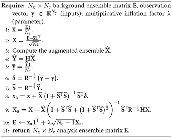
Algorithm 1. Analysis step for a generic LEnSRF used in this article. The augmented ensemble at step 3 can be constructed using the modulation method with or without the balanced refinement or using the truncated svd method.
4. Accuracy of the Approximate Factorisation
4.1. A Simple One-Dimensional Model for the Background Error Covariance Matrix
In this section, we investigate the accuracy of the factorisation Equation (18) obtained with the methods described in section 3.2. The background error covariance matrix is obtained as follows.
Let G be the piecewise rational function of Gaspari and Cohn [33]. Let d be the Euclidean distance over the set {1…Nx} with periodic boundary conditions. For any radius r ∈ ℝ+, we define C(r) as the Nx × Nx matrix whose coefficients satisfy
For any vector , we define as the Nx × Nx diagonal matrix whose diagonal is precisely .
We draw a vector c from the distribution , where αc and rc are two parameters. We define:
Cref plays the role of a reference covariance matrix in our model. We now draw a sample of Ne independent members from the distribution . Without loss of generality, we assume that the associated ensemble matrix X is normalised by . We define the background error covariance matrix as
with the localisation matrix ρ = C(rref).
4.2. Experimental Setup
In the following test series, we use two matrices B1 and B2. They are constructed using different realisations of the model described in section 4.1 with the parameters specified in Table 1. Note that we used short-range correlations (rref = 20) to construct B1 and mid-range correlations (rref = 100) to construct B2. Figure 1 displays the matrices B1 and B2.
TABLE 1
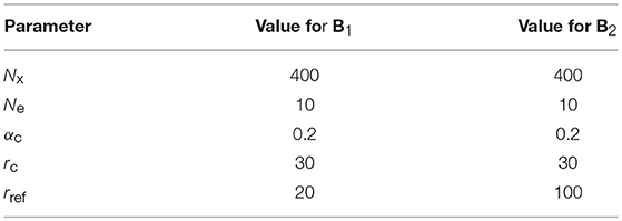
Table 1. Parameters used to construct B1 and B2 with the model described in section.
FIGURE 1
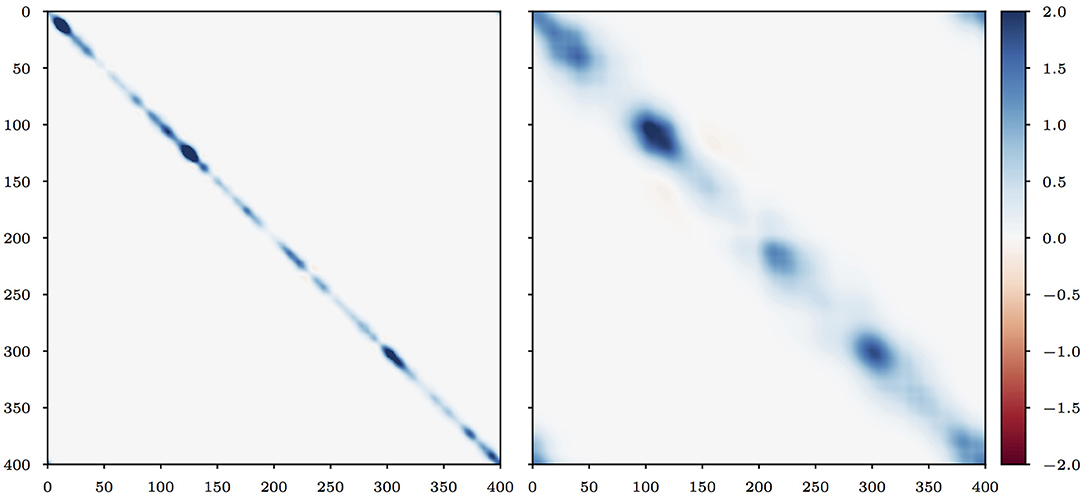
Figure 1. Background error covariance matrices B1 (left) and B2 (right).
The modulation method described in sections 3.2.2 and 3.2.3 requires an approximate factorisation for ρ = C(rref), that we precompute by keeping the first Nm or Nm + δNm (when using the balance refinement) modes in the svd of ρ. Since ρ is sparse, we use the random svd (Algorithm 2) to obtain this factorisation.
4.3. Results and Discussion
We apply the methods described in section 3.2 to obtain an approximate factorisation for B1 and B2 and we compute the normalised Frobenius error:
Using the Eckart–Young theorem [34], we conclude that the lowest normalised Frobenius error for a factorisation with rank is
where σk(M) is the k-th singular value of the matrix M.
Figure 2 shows the evolution of the normalised Frobenius error eF, i as a function of the augmented ensemble size when the factorisation is computed using the truncated svd method (section 3.2.4) or the modulation method with (section 3.2.3) or without (section 3.2.2) the balance refinement. The value reported for eF, i is the average value over 100 independent realisations of the random svd. For q ≥ 1, the Frobenius error of the truncated svd method (not shown here) cannot be distinguised from the minimum possible value. For the modulation method, using the balance refinement with δNm > 10 (not shown here) does not yield a clear improvement over the case δNm = 10. The singular values of B2 (mid-range case) decay much faster than the singular values of B1 (short-range case). This explains why the normalised Frobenius errors eF, 2 are systematically lower than the normalised Frobenius errors eF, 1.
FIGURE 2
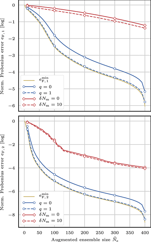
Figure 2. Evolution of the normalised Frobenius errors eF, 1 (top) and eF, 2 (bottom) as a function of the augmented ensemble size . The approximate factorisation of B1 (top) and B2 (bottom) is computed either using the truncated svd method with several values for the parameter q for the random svd Algorithm 2 (blue lines) or using the modulation method with (solid red line) or without (dashed red line) the balance refinement. The lowest normalised achievable Frobenius errors are plotted in yellow for both cases.
The modulation method is very fast but yields a poor approximation of the background error covariance matrix B. With the balance refinement, the approximation is a bit better and the method is still very fast. By contrast, the truncated svd method is much slower but yields an approximation of B close to optimal. At this point, it is not clear what level of precision is needed for B. Yet, we can already conclude that, in a cycled DA context, we will have to find a balance between speed and accuracy in the construction of the augmented ensemble and in the perturbation update.
Finally, different matrix norms could have been used in this test series. Indeed, even if equivalent, two matrix norms give different informations. This is why we have computed the normalised spectral error (not shown here) and found quite similar results to those depicted in Figure 2. This shows that our results are not specific to the Frobenius norm.
5. Cycled DA Experiments With a One-Dimensional Model
5.1. The Lorenz 1996 Model
The L96 model [24] is a low-order one-dimensional discrete model whose evolution is given by the following ordinary differential equations (ODEs):
where the indices are to be understood with periodic boundary conditions: x−1 = xNx−1, x0 = xNx, x1 = xNx+1 and where the system size Nx can take arbitrary values. These ODEs are integrated using a fourth-order Runge–Kutta method with a time step of 0.05 time unit.
The standard configuration Nx = 40 and F = 8 is widely used in DA to assess the performance of the DA algorithms. It yields chaotic dynamics with a doubling time around 0.42 time unit. In this section, we use an extended standard configuration where Nx = 400 and F = 8, which is essentially a repetition of ten times the standard configuration. The observations are given by
and the time interval between consecutive observations is Δt = 0.05 time unit, which represents 6 h of real time and corresponds to a model autocorrelation around 0.967. The standard deviation of the observation noise is approximately one tenth of the climatological variability of each observation.
For the localisation, we use the Euclidean distance over the set {1…Nx} with periodic boundary conditions (the same as the one that was used in section 4).
Note that we use Nx = 400 state variables instead of 40 such that typical local domains (with a localisation radius around r = 20 grid points) do not cover the whole domain.
5.2. Experimental Setup
In this section, we illustrate the performance of the LEnSRF Algorithm 1 using twin simulations of the L96 model in the extended configuration. The augmented ensemble (step 3 of Algorithm 1) is computed using the truncated svd method (section 3.2.4) or the modulation method with (section 3.2.3) or without (section 3.2.2) the balance refinement. Both methods use an ensemble of Ne = 10 members and a localisation matrix ρ = C(r), where the localisation radius r is a free parameter.
For the modulation method, the approximate factorisation of ρ is precomputed once for each twin experiment by keeping the first Nm or Nm + δNm (when using the balance refinement) modes in the svd of ρ.
For the truncated svd method, the matrix multiplications implying B are computed using Equation (30) and ρ is applied in spectral space.
The runs are 2 × 10⁴Δt long (with an additional 2 × 10³Δt spin-up period) and our performance criterion is the time-average analysis root mean square error, hereafter called the RMSE.
5.3. Augmented Ensemble Size—RMSE Evolution
Figure 3 shows the evolution of the RMSE as a function of the augmented ensemble size . Both the truncated svd and the modulation methods are able to produce an estime of the true state with an accuracy equivalent to that of the local ensemble transform Kalman filter (LETKF, [35]). As expected after the experiments in section 4, for a given level of RMSE score we need a much smaller augmented ensemble size when using the truncated svd method than when using the modulation method. However, before we conclude that the truncated svd method is more efficient, we need to take into account the fact that computing the augmented ensemble is much slower with this method than with the modulation method.
FIGURE 3
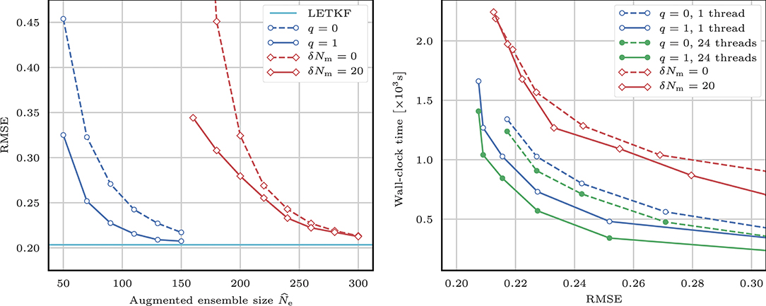
Figure 3. Evolution of the RMSE as a function of the augmented ensemble size (left) and of the wall-clock analysis time for the 22 × 103 cycles as a function of the RMSE for the LEnSRF Algorithm 1. For each data point, the localisation radius r and the inflation factor λ are optimally tuned to yield the lowest RMSE. The augmented ensemble is computed either using the truncated svd method with several values for the parameter q in the random svd Algorithm 2 (green and blue lines) or using the modulation method with (solid red line) or without (dashed red line) the balance refinement. In the left panel, the horizontal solid cyan baseline is the RMSE of the LETKF with an ensemble of Ne = 10 members and optimally tuned localisation radius r and inflation factor λ.
With the truncated svd method, the augmented ensemble size needs to be at least of the same order as the number of unstable and neutral modes of the model dynamics (around 133 here) in order to yield accurate results [4]. We have also tested q > 1 in the truncated svd method or δNm > 20 in the modulation method (not shown here) and found that none of these parameters yields clear improvements in RMSE scores.
5.4. RMSE—Wall-Clock Time Evolution
The longest algorithmic operations in Algorithm 1 are:
1. constructing the augmented ensemble (step 3);
2. computing the svd of (required for steps 8 and 9);
When using the truncated svd method, some level of parallelisation can be included in the construction of the augmented ensemble as remarked in Appendix B.2. When using the modulation method (even with the balance refinement), constructing the augmented ensemble is almost instantaneous compared to computing the svd of . Therefore, we only enable parallelisation when using the truncated svd method.
To compute the analysis state and analysis perturbations Xa, we have tested several approaches and concluded that the most efficient is to compute the svd of with a direct svd algorithm, which cannot be parallelised.
Figure 3 shows the evolution of the wall-clock time of one analysis step as a function of the RMSE. All simulations are performed on the same double Intel Xeon E5-2680 platform, which has a total of 24 cores. Parallelisation is enabled when possible using a fixed number of OpenMP threads. For a given level of RMSE score, the truncated svd method is clearly faster than the modulation method. This shows the advantage of using the truncated svd method over the modulation method, especially when parallelisation is possible. However, this result is specific to the problem considered in this section and may not generalise to all situations.
6. Cycled DA Experiments With Satellite Radiances
6.1. Is Covariance Localisation Viable With High-Dimensional Models?
In section 5, we have implemented covariance localisation in the EnKF and successfully applied the resulting algorithm to a one-dimensional DA problem with Nx = 400 state variables. With a high-dimensional system, covariance localisation in the EnKF will probably require a very large augmented ensemble size , too large to be affordable. In this case, the use of domain localisation will be mandatory.
When observations are local, domain localisation is simple to implement and yield efficient algorithms such as the LETKF. However, when observations are non-local, one must resort to ad hoc approximations to implement domain localisation in the EnKF, for example assigning an approximate location to each observation. In this section, we discuss the case of satellite radiances, which are non-local observations and we show how existing variants of the LETKF deal with such observations. We then give an extension of our LEnSRF Algorithm 1 designed to assimilate satellite radiances in a spatially extended model. Finally we introduce a multilayer extension of the L96 model that mimics satellite radiances and we illustrate the performance of our method using twin simulations of this model.
6.2. The Case of Satellite Radiances
Suppose that the physical space consists of a multilayer space with Pz vertical levels of Ph state variables. For any h ∈ {1…Ph} and z ∈ {1…Pz}, the state variable located at the h-th horizontal position and at the z-th vertical level is written x(z, h). For any state vector x, the sub-vector of the components located at the h-th horizontal position at any level is written xh and called the h-th column of x.
Suppose that each state vector column is observed independently via
where Ω is a Pc × Pz weighting matrix and is the vector containing the Pc observations at the h-th horizontal position. Pc is the number of channels. The full observation vector is the concatenation of all . It has Ny = Pc × Ph components and for any h ∈ {1…Ph} and c ∈ {1…Pc}, the observation located at the h-th horizontal position and corresponding to the c-th channel is written y(c, h).
This simple model describes a typical situation for satellite radiances. From these definitions, it is clear that each observation is attached to an horizontal position, but has no well-defined vertical position (unless the weighting matrix Ω is diagonal). Several variants of the LETKF have been designed to assimilate such observations. When the weighting function of a channel has a single and well-located maximum, the vertical location of this maximum can play the role of an approximate height for this channel. This is the approach followed for example by Fertig et al. [11]. Based on these vertical positions, they use the channels to update “adjacent” vertical levels as long as the corresponding weighting function is above a threshold value. Campbell et al. [9] has followed the same approach to define the approximate height of the channels. However their update formula includes a vertical tapering of the anomalies that depends on the vertical distance. When the weighting functions are flat, another possibility is to define the approximate height of a channel as the middle of the support of its weighting function [36]. Miyoshi and Sato [10] have proposed an alternative that does not require the definition of an approximate height of the channels: their update formula includes a vertical tapering of the anomalies that depends on the shape of the weight functions only. Finally, in the algorithm of Penny et al. [37], vertical localisation has been removed.
Using a realistic one-dimensional model with satellite radiances, Campbell et al. [9] have shown that ad hoc approaches based on domain localisation only systematically yield higher errors than covariance localisation. In a spatially extended model with satellite radiances, it seems natural to apply domain localisation in the horizontal direction, in which observations are local, while using covariance localisation in the vertical direction, in which observations are non-local.
6.3. Including Domain Localisation in the LEnSRF
Following the approach of Bishop et al. [19], we apply four modifications to the generic LEnSRF Algorithm 1 in order to include domain localisation in way similar to the LETKF.
1. We perform Ph local analyses instead of one global analysis. The aim of the h-th local analysis is to give an update for the Pz state variables that form the h-th column. The linear algebra must be adapted in consequence.
2. We taper the anomalies related to each observation with respect to the horizontal distance to the h-th column. This is usually implemented in .
3. Observations whose horizontal position is far from the h-th column (i.e., observations that are not in the local domain) do not contribute to the update. These observations are therefore omitted in the local analysis in order to save some computational time.
4. Since observations that are outside of the local domain are omitted, we only need to compute an augmented ensemble for the state variables inside the local domain. Since covariance localisation is only applied in the vertical direction, the augmented ensemble must have empirical covariance matrix given by
where Xℓ is the set of perturbations that are located within the local domain and ρv is the vertical localisation matrix, whose coefficients only depend on the vertical layer indices.
This modified LEnSRF, hereafter called local analysis LEnSRF (L2EnSRF), implements domain localisation in the horizontal direction and covariance localisation in the vertical direction and therefore can be used to assimilate vertically non-local observations such as satellite radiances.
6.4. The Multilayer L96 Model
We now introduce a multilayer extension of the L96 model, hereafter called mL96 model. This multilayer extension is used to test and illustrate the performance of the L2EnSRF algorithm.
The mL96 model consists of Pz coupled layers of the one-dimensional L96 model with Ph variables. Keeping the notations defined in section 6.2, the evolution of the model is given by the following PzPh ODEs:
The first line of Equation (50) corresponds to the original L96 ODE Equation (46), with a forcing term that may depend on the vertical layer index z. The second and third lines correspond to the coupling between adjacent layers, with a constant intensity Γ. As for the L96, the horizontal indices are to be understood with periodic boundary conditions: x(z, −1) = x(z, Ph−1), x(z, 0) = x(z, Ph), and x(z, 1) = x(z, Ph+1). These ODEs are integrated using a fourth-order Runge–Kutta method with a time step of 0.05 time unit.
For this experiment, we use Pz = 32 layers and Ph = 40 to mimic the standard configuration of the L96 model. The forcing term linearly decreases from F1 = 8 at the lowest level to FPz = 4 at the highest level. Without the coupling, these values would render the lower levels dynamics chaotic and the higher levels dynamics laminar, which is a typical behaviour in the atmosphere. Finally, we take Γ = 1 such that adjacent layers are highly correlated (correlation around 0.87). To be more specific, the correlation between the z-th level and the (z + δz)-th level first rapidly decreases with δz. It reaches approximately −0.1 for δz = 6 and then it starts increasing. Finally, its absolute value is below 10−2 when δz > 10. This model is chaotic and the dimension of the unstable or neutral subspace is around 50.
The observation operator H follows the model described in section 6.2. We use Pc = 8 channels and a weighting matrix Ω designed to mimic satellite radiances as shown in Figure 4. The observations are given by
and the time interval between consecutive observations is the same as the one used with the L96 model, Δt = 0.05 time unit. Once again, the standard deviation of the observation noise is approximately one tenth of the climatological variability of each observation.
FIGURE 4
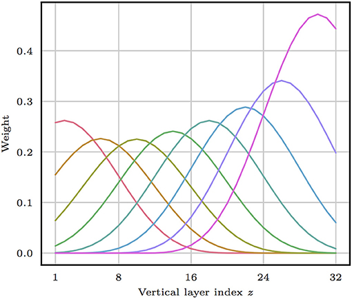
Figure 4. Observation operator H. Each line represents the weighting function of a different channel, corresponding to a row of the weighting matrix Ω. Every channel has a single maximum and is relatively broad (half-width around 10 vertical layers). The sum of the weights has been adjusted individually such that every channel yields an observation with approximately the same climatological variability.
For the horizontal localisation, we use the Euclidean distance dh over the set {1…Ph} with periodic boundary conditions. For the vertical localisation, we use the Euclidean distance dv over the set {1…Pz}.
6.5. Experimental Setup
In this section, we give some details on how localisation is implemented in the L2EnSRF algorithm for the mL96 model. We then described which approximations are made to implement an LETKF algorithm. For each algorithm, the runs are 104Δt long (with an additional 103Δt spin-up period) and our performance criterion is the time-average analysis RMSE.
6.5.1. Horizontal Localisation
Let rh be the horizontal localisation radius. During the h1-th local analysis, the anomalies related to observation y(c,h2) are tapered by a factor
where G is the piecewise rational function of Gaspari and Cohn [33]. This means that the h-th local domain consists of the columns {h− ⌊rh…h⌋ + ⌊rh⌋} where the indices are to be understood with Ph periodic boundary conditions and ⌊rh⌋ is the integer part of rh.
6.5.2. Vertical Localisation
Let rv be the vertical localisation radius. The vertical localisation matrix ρv has coefficients given by
The local domain gathers columns, hence ρv is a block-diagonal matrix. Since its coefficients only depend on the vertical layer indices, it can also be seen as a Pz × Pz matrix.
The matrix of the augmented ensemble is computed using the truncated svd method (section 3.2.4) or the modulation method with (section 3.2.3) or without (section 3.2.2) the balance refinement. Both methods use an ensemble of Ne = 8 members and the localisation matrix ρv.
For the modulation method, the approximate factorisation of ρv is precomputed once for each twin experiment by keeping the first Nm or Nm+δNm (when using the balance refinement) modes in the svd of the Pz × Pz matrix ρv.
For the truncated svd method, the matrix multiplications implying B are computed using Equation (30). Because the coefficients of the localisation matrix ρv only depends on the vertical layer indices, applying the matrix ρv to a vector with components reduces to applying the Pz × Pz matrix ρv to a vector with Pz components. It should be relatively quick and therefore we do not perform this product in spectral space. This means that the implementation can be straightforwardly adapted to the general case where the vertical layers are not equally distributed in height.
6.5.3. Ad hoc Approximations for the LETKF
We define an approximate height zc for the c-th channel:
We did not define zc as the vertical position of the maximum of the c-th weight function because we wanted to account for the fact that our weight functions are skewed in the vertical direction.
In the LETKF algorithm, we perform PzPh local analyses (one for each state variable). In the local analysis for the state variable x(z,h1), the anomalies related to observation y(c,h2) are tapered by a factor
where
and rh and rv are the horizontal and vertical localisation radii, respectively.
6.6. Results
Figure 5 shows the evolution of the RMSE and of the wall-clock time of one analysis step as a function of the horizontal localisation radius rh for the L2EnSRF and the LETKF. All simulations are performed on the same double Intel Xeon E5-2680 platform, which has a total of 24 cores. Parallelisation is enabled for the Ph independent local analyses using a fixed number of OpenMP threads Nthr = 20. In the L2EnSRF algorithm, the augmented ensemble is computed either using the truncated svd method with q = 0 in the random svd (Algorithm 2) or using the modulation method without the balance refinement (δNm = 0). Preliminary experiments with q > 0 or δNm > 0 (not shown here) did not display clear improvements in RMSE score over the cases q = 0 and δNm = 0.
FIGURE 5
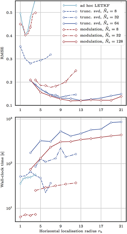
Figure 5. Evolution of the RMSE (top) and of the wall-clock analysis time for the 103 cycles (bottom) as a function of the horizontal localisation radius rh for the L2EnSRF algorithm. For each data point, the vertical localisation radius rv and the inflation factor λ are optimally tuned to yield the lowest RMSE. The augmented ensemble is computed either using the truncated svd method (blue lines) with q = 0 in the random svd Algorithm 2 or using the modulation method (red lines) without the balance refinement (ΔNm = 0). As a reference, we draw the same data for the LETKF with the ad hoc approximations described in section 6.5.3 (cyan line).
The LETKF produces rather high RMSE scores (compare to the standard deviation of the observation noise, which is 1), while not completely failing to reconstruct the true state. Although domain localisation in the horizontal direction is a powerful tool, vertical localisation is necessary in this DA problem. Because the weight functions of the channels are quite broad, observations cannot be considered local and domain localisation in the vertical direction is inefficient. By contrast, with a reasonable augmented ensemble size , the L2EnSRF yields significantly lower RMSEs. This shows that combining domain localisation in the horizontal direction and covariance localisation in the vertical direction is an adequate approach to assimilate satellite radiances.
The comparison between the truncated svd and the modulation methods is not as simple as it was in the L96 test series. As expected, for a given augmented ensemble size , the truncated svd method yields lower RMSE scores. However, for a given level of RMSE score, using the truncated svd method is not always the fastest approach. For example, the RMSE of the truncated svd method with is approximately the same as the RMSE of the modulation method with , but in this case the modulation method is faster by a factor 1.5 on average. This can be explained by two factors. First, in the truncated svd method the vertical localisation matrix is not applied in spectral space. Second, both the truncated svd and the modulation method benefit from parallelisation, but the parallelisation potential of the truncated svd method is not fully exploited here because our computational platform has a limited number of cores. This would change if we could use several threads for each local analysis. Finally, these results confirm that, for high dimensionals DA problems where the memory requirement is an issue, the truncated svd method is the best approach to obtain accurate results while using only a limited augmented ensemble size .
7. Conclusions
Localisation is widely used in DA to make the EnKF viable in high-dimensional systems. In the EnKF, two different approaches can be used to include localisation: domain localisation or covariance localisation. In this article, we have explored possible implementations for covariance localisation in the deterministic EnKF using augmented ensembles in the analysis step. We have discussed the two main difficulties related to augmented ensembles: how to construct the augmented ensemble and how to update the perturbations.
We have used two different methods to construct the augmented ensemble. The first one is based on a factorisation property of the background error covariance matrix. It is already widespread in the geophysical DA literature under the name modulation. For this method, we also introduced a balance refinement in order to smooth some variability between the state variables. As an alternative, we proposed a second method based on randomised svd techniques, which are very efficient when the localisation matrix is easy to apply. The random svd algorithm is commonly used in the statistical literature but it had never been applied in this context. We have called this approach truncated svd method.
We have shown how covariance localisation can be included in the perturbation update using the augmented ensemble framework. The resulting update formula [18] uses linear algebra in the augmented ensemble space. It is included in the generic LEnSRF detailed in this article.
Using numerical simulations of a very simple one-dimensional covariance model with 400 state variables, we have shown that the truncated svd method yields a much more accurate approximation of the background covariance than the modulation method. This result has been confirmed by twin simulations of the one-dimension L96 model with 400 variables. In a standard DA setup, we have found that the balance between fast computation of the augmented ensemble and fast perturbation update is in favor of the truncated svd method. In other words, for a given level of RMSE score, it is worth spending more time to construct a smaller but more reliable augmented ensemble with the truncated svd method and then use a fast perturbation update.
We have defined the L2EnSRF algorithm as an extension of the LEnSRF suited to assimilate satellite radiances in spatially extended models. It implements domain localisation in the horizontal direction in a similar way as the LETKF and covariance localisation in the vertical direction. Such an extension had been discussed by Bishop et al. [19] but without numerical illustration.
Finally, we have constructed a simple multilayer extension of the L96 model, called mL96 model. We have performed twin simulations of this model using a satellite-like observation operator. As expected, the LETKF hardly reconstructs the true state. By contrast, the L2EnSRF yields an estimate of the true state with an acceptable accuracy. We have concluded that using domain localisation in the horizontal direction and covariance localisation in the vertical direction is an adequate approach to assimilate satellite radiances in a spatially extended model. For a given level of RMSE score, the modulation method is the fastest approach in this DA problem. This result is however mitigated by the fact that our computational setup does not use the full parallelisation potential of the truncated svd method. However, when the augmented ensemble size is limited, the truncated svd method is the best approach to obtain accurate results.
Author Contributions
All authors have made a substantial, direct and intellectual contribution to the work, and approved it for publication.
Conflict of Interest Statement
The authors declare that the research was conducted in the absence of any commercial or financial relationships that could be construed as a potential conflict of interest.
Acknowledgments
CEREA is a member of Institut Pierre–Simon Laplace (IPSL). MB acknowledges early discussions with N. Bousserez on the randomised svd techniques.
References
1. Evensen G. Sequential data assimilation with a nonlinear quasi-geostrophic model using Monte Carlo methods to forecast error statistics. J Geophys Res. (1994) 99:10143–62. doi: 10.1029/94JC00572
2. Houtekamer PL, Mitchell HL, Pellerin G, Buehner M, Charron M, Spacek L, et al. Atmospheric data assimilation with an ensemble Kalman filter: results with real observations. Mon Weather Rev. (2005) 133:604–20. doi: 10.1175/MWR-2864.1
3. Sakov P, Counillon F, Bertino L, Lisæter KA, Oke PR, Korablev A. TOPAZ4: an ocean-sea ice data assimilation system for the North Atlantic and Arctic. Ocean Sci. (2012) 8:633–56. doi: 10.5194/os-8-633-2012
4. Bocquet M, Carrassi A. Four-dimensional ensemble variational data assimilation and the unstable subspace. Tellus B (2017) 69:1304504. doi: 10.1080/16000870.2017.1304504
5. Houtekamer PL, Mitchell HL. A sequential ensemble Kalman filter for atmospheric data assimilation. Mon Weather Rev. (2001) 129:123–37. doi: 10.1175/1520-0493(2001)129<0123:ASEKFF>2.0.CO;2
6. Ott E, Hunt BR, Szunyogh I, Zimin AV, Kostelich EJ, Corazza M, et al. A local ensemble Kalman filter for atmospheric data assimilation. Tellus B (2004) 56:415–28. doi: 10.1111/j.1600-0870.2004.00076.x
7. Hamill TM, Whitaker JS, Snyder C. Distance-dependent filtering of background error covariance estimates in an ensemble Kalman filter. Mon Weather Rev. (2001) 129:2776–90. doi: 10.1175/1520-0493(2001)129<2776:DDFOBE>2.0.CO;2
8. Sakov P, Bertino L. Relation between two common localisation methods for the EnKF. Computat Geosci. (2011) 15:225–37. doi: 10.1007/s10596-010-9202-6
9. Campbell WF, Bishop CH, Hodyss D. Vertical covariance localization for satellite radiances in ensemble Kalman filters. Mon Weather Rev. (2010) 138:282–90. doi: 10.1175/2009MWR3017.1
10. Miyoshi T, Sato Y. Assimilating satellite radiances with a local ensemble transform Kalman filter (LETKF) applied to the JMA global model (GSM). SOLA (2007) 3:37–40. doi: 10.2151/sola.2007-010
11. Fertig EJ, Hunt BR, Ott E, Szunyogh I. Assimilating non-local observations with a local ensemble Kalman filter. Tellus B (2007) 59:719–30. doi: 10.1111/j.1600-0870.2007.00260.x
12. Buehner M. Ensemble-derived stationary and flow-dependent background-error covariances: evaluation in a quasi-operational NWP setting. Q J Roy Meteor Soc. (2005) 131:1013–43. doi: 10.1256/qj.04.15
13. Lorenc AC. The potential of the ensemble Kalman filter for NWP-a comparison with 4D-Var. Q J Roy Meteor Soc. (2003) 129:3183–203. doi: 10.1256/qj.02.132
14. Bishop CH, Hodyss D. Ensemble covariances adaptively localized with ECO-RAP. Part 2: a strategy for the atmosphere. Tellus B (2009) 61:97–111. doi: 10.1111/j.1600-0870.2008.00372.x
15. Brankart JM, Cosme E, Testut CE, Brasseur P, Verron J. Efficient local error parameterizations for square root or ensemble Kalman filters: application to a basin-scale ocean turbulent flow. Mon Weather Rev. (2011) 139:474–93. doi: 10.1175/2010MWR3310.1
16. Bishop CH, Hodyss D. Adaptive ensemble covariance localization in ensemble 4D-VAR state estimation. Mon Weather Rev. (2011) 139:1241–55. doi: 10.1175/2010MWR3403.1
17. Leng H, Song J, Lu F, Cao X. A new data assimilation scheme: the space-expanded ensemble localization Kalman filter. Adv Meteorol. (2013) 2013:410812. doi: 10.1155/2013/410812
18. Bocquet M. Localization and the iterative ensemble Kalman smoother. Q J Roy Meteor Soc. (2016) 142:1075–89. doi: 10.1002/qj.2711
19. Bishop CH, Whitaker JS, Lei L. Gain form of the ensemble transform Kalman filter and its relevance to satellite data assimilation with model space ensemble covariance localization. Mon Weather Rev. (2017) 145:4575–92. doi: 10.1175/MWR-D-17-0102.1
20. Kretschmer M, Hunt BR, Ott E. Data assimilation using a climatologically augmented local ensemble transform Kalman filter. Tellus B (2015) 67:26617. doi: 10.3402/tellusa.v67.26617
21. Bishop CH, Etherton BJ, Majumdar SJ. Adaptive sampling with the ensemble transform Kalman filter. Part I: theoretical aspects. Mon Weather Rev. (2001) 129:420–36. doi: 10.1175/1520-0493(2001)129<0420:ASWTET>2.0.CO;2
22. Lorenc AC. Improving ensemble covariances in hybrid variational data assimilation without increasing ensemble size. Q J Roy Meteor Soc. (2017) 143:1062–72. doi: 10.1002/qj.2990
23. Halko N, Martinsson PG, Tropp JA. Finding structure with randomness: probabilistic algorithms for constructing approximate matrix decompositions. SIAM Rev. (2011) 53:217–88. doi: 10.1137/090771806
24. Lorenz EN, Emanuel KA. Optimal sites for supplementary weather observations: simulation with a small model. J Atmos Sci. (1998) 55:399–414. doi: 10.1175/1520-0469(1998)055<0399:OSFSWO>2.0.CO;2
25. Evensen G. Data Assimilation: The Ensemble Kalman Filter. Berlin; Heidelberg: Springer-Verlag (2009).
27. Sakov P, Oke PR. A deterministic formulation of the ensemble Kalman filter: an alternative to ensemble square root filters. Tellus B (2008) 60:361–71. doi: 10.1111/j.1600-0870.2007.00299.x
28. Whitaker JS, Hamill TM. Ensemble data assimilation without perturbed observations. Mon Weather Rev. (2002) 130:1913–24. doi: 10.1175/1520-0493(2002)130<1913:EDAWPO>2.0.CO;2
29. Desroziers G, Camino JT, Berre L. 4DEnVar: link with 4D state formulation of variational assimilation and different possible implementations. Q J Roy Meteor Soc. (2014) 140:2097–110. doi: 10.1002/qj.2325
30. Desroziers G, Arbogast É, Berre L. Improving spatial localization in 4DEnVar. Q J Roy Meteor Soc. (2016) 142:3171–85. doi: 10.1002/qj.2898
31. Arbogast É, Desroziers G, Berre L. A parallel implementation of a 4DEnVar ensemble. Q J Roy Meteor Soc. (2017) 143:2073–83. doi: 10.1002/qj.3061
32. Peres-Neto PR, Jackson DA, Somers KM. How many principal components? Stopping rules for determining the number of non-trivial axes revisited. Comput Stat Data Ann. (2005) 49:974–97. doi: 10.1016/j.csda.2004.06.015
33. Gaspari G, Cohn SE. Construction of correlation functions in two and three dimensions. Q J Roy Meteor Soc. (1999) 125:723–57. doi: 10.1002/qj.49712555417
34. Eckart C, Young G. The approximation of one matrix by another of lower rank. Psychometrika (1936) 1:211–8. doi: 10.1007/BF02288367
35. Hunt BR, Kostelich EJ, Szunyogh I. Efficient data assimilation for spatiotemporal chaos: a local ensemble transform Kalman filter. Phys D (2007) 230:112–26. doi: 10.1016/j.physd.2006.11.008
36. Anderson J, Lei L. Empirical localization of observation impact in ensemble Kalman filters. Mon Weather Rev. (2013) 141:4140–53. doi: 10.1175/MWR-D-12-00330.1
37. Penny SG, Behringer DW, Carton JA, Kalnay E. A hybrid global ocean data assimilation system at NCEP. Mon Weather Rev. (2015) 143:4660–77. doi: 10.1175/MWR-D-14-00376.1
Appendix
A. Recentre the Perturbations
Let X be an Nx × (Ne − 1) matrix. We want to construct a matrix that has the same empirical covariance matrix and which is centred. Since X has rank at most Ne − 1, we need to find an Nx × Ne matrix Z such that
For ϵ ∈ {−1, 1}, we define and Qϵ as the Ne × Ne matrix whose coefficients are
It can be easily checked that (i.e., Qϵ is an orthogonal matrix) and , the first basis vector.
Let W be the Nx × Ne matrix whose first column is zero and whose other columns are those of X, that is
By construction Z = WQϵ is a solution of Equations (A1) and (A2).
B. A Random svd Algorithm
B.1. The Algorithm
Algorithm 2 describes the random svd algorithm proposed by Halko et al. [23]. The objective of this algorithm is to efficiently compute an approximate truncated svd with P columns of the M × N matrix A as a parallelisable alternative to Lanczos techniques.
The random svd algorithm is based on two ideas. First, suppose that there is a matrix Q with P orthonormal columns which approximates the range of the matrix A. In other words A ≈ QQT A. Then, an approximate truncated svd can be obtained for A using the svd of the smaller matrix QT A. Second, the matrix Q can be constructed using random draws. Indeed, if is a set of random vectors, then it is most likely a linearly independant set. Therefore, the set is most likely linearly independant, which means that it spans the range of A.
One major contribution of Halko et al. [23] and the references therein is that they have provided a mathematical justification of these ideas. In particular, they have given statistical performance bounds for the random svd algorithm and emphasised the fact that, on average, the (spectral or Frobenius) error of the resulting truncated svd with P columns should be close to the minimal error for a truncated svd with P columns.
Finally, Halko et al. [23] have introduced two elements to improve the numerical stability and efficiency of the random svd algorithm. The first element is a loop over i ∈ {1…q}, which forces the algorithm to construct singular vectors of (AAT)q A instead of A. However, (AAT)q A and A share the same singular vectors. Moreover, the singular values of (AAT)q A decay faster than those of A, which means that this technique enables a better approximation of the decomposition as shown by Corollary 10.10 of Halko et al. [23]. The second element is to include QR factorisations to make the algorithm less vulnerable to round-off errors. Both elements have been taken into account in Algorithm 2.
ALGORITHM 2
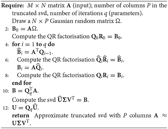
Algorithm 2. Random svd algorithm
B.2. Application to the Prior Covariance Matrix
In section 3.2.4, we need to compute the truncated svd Equation (26) of the prior covariance matrix. To do this, we can apply Algorithm 2 using the input matrix A = ρ∘ (XXT). The prior covariance matrix is a large Nx × Nx matrix. However, Algorithm 2 can work with the map
which can be efficiently computed using Equation (30). Steps 2, 5, 7, and 10 of Algorithm 2 can even be parallelised by applying A = ρ ∘ (XXT) independently to each column.
Finally, the approximate truncated svd
resulting from Algorithm 2 does not necessarily satisfy U = V even though the input matrix is symmetric positive definite. The simplest fix is to make the additional approximation
Keywords: ensemble Kalman filter, covariance localisation, modulation, random svd, satellite radiances, non-local observations
Citation: Farchi A and Bocquet M (2019) On the Efficiency of Covariance Localisation of the Ensemble Kalman Filter Using Augmented Ensembles. Front. Appl. Math. Stat. 5:3. doi: 10.3389/fams.2019.00003
Received: 08 November 2018; Accepted: 14 January 2019;
Published: 26 February 2019.
Edited by:
Ulrich Parlitz, Max-Planck-Institute for Dynamics and Self-Organisation, Max Planck Society (MPG), GermanyReviewed by:
Peter Jan Van Leeuwen, University of Reading, United KingdomXin Tong, National University of Singapore, Singapore
Copyright © 2019 Farchi and Bocquet. This is an open-access article distributed under the terms of the Creative Commons Attribution License (CC BY). The use, distribution or reproduction in other forums is permitted, provided the original author(s) and the copyright owner(s) are credited and that the original publication in this journal is cited, in accordance with accepted academic practice. No use, distribution or reproduction is permitted which does not comply with these terms.
*Correspondence: Alban Farchi, alban.farchi@enpc.fr