- 1Graduate School of Economics, Osaka University, Osaka, Japan
- 2Department of Economics, Meiji Gakuin University, Tokyo, Japan
The study of intertemporal decision-making is an interdisciplinary scientific topic of economics, psychology, and neuroscience. Most of these studies focus on individual intertemporal decisions, but little is known about the relationship between groups and individual time preferences. As a result, we intend to assess the role of group intertemporal decision-making. We experimentally investigate how to aggregate individual time preferences by clarifying who has the most influence on group decisions among heterogeneous group members. We formulate two hypotheses. The first is the multilateral bargaining hypothesis, which is based on the multilateral bargaining model. If people employ this model to reach agreement, the most patient member in a group has the greatest impact on group choices. The second is the median voter hypothesis, which is based on the median voter model. When people employ this model to reach agreement, the median patient member in a group has the greatest impact on group choices. Here, we find that the median patient member in a group has a significant impact on group decisions in an unstructured bargaining situation. This finding suggests that people use the majority voting rule during group intertemporal decision-making. Thus, our findings support the median voter hypothesis. Furthermore, the results of a chat analysis show that this result is partially due to people's conformity with the majority opinion.
Introduction
Many essential economic decisions are made by groups such as companies and households. For example, investment plans in companies are decided in meetings with multiple people, and saving plans in households are decided by partners. Environmental decisions are also intertemporal choices. For example, we are faced with a decision between consuming ecological resources today vs. enjoying a rich environment later. These types of decisions are mainly made by the society, such as local communities, governments, and so on.
In general, economists describe a group choice as a summation of individual choices or representative individuals. Do real-life group decisions over time work in this way? Although it is important that we understand how intertemporal group decision are made, there is little empirical evidence on the relationship between group and individual time preferences. Very few studies have used experiments to examine groups' intertemporal choices1. Yang and Carlsson [2] investigated whether a group consensus related to intertemporal decision-making was derived from individual time preferences. In their research, participants were wives and husbands in rural China, where each couple answered intertemporal questions. They found that 11% of the consensus decisions made by couples were more patient than both the wife's and husband's individual choices and that 9% of the consensus decisions were more impatient than the individuals' choices. Interestingly, their result suggested that some proportion of group consensus decisions were not simply a summation of individuals' choices. Nevertheless, they failed to reveal why couples' consensus decisions were beyond the individuals' time preferences. Furthermore, they focused on family financial decisions made by spouses. Thus, we cannot apply their findings to groups' intertemporal choices in general. Yang and Carlsson [2] and Carlsson et al. [3] also investigated who in the family had the most influence on group consensus decisions, identifying that husbands had a greater impact than wives did in joint choices. However, this result could be culture specific and, thus, might not be generalizable to other regions or countries.
The purpose of this study is to investigate the mechanism behind groups' intertemporal decision-making in heterogeneous time preferences by clarifying who has a significant impact on groups' intertemporal choices. As such, we contribute to the literature by investigating the difference between group preferences and individual preferences. Charness and Sutter [4] indicate that groups make more self-interested decisions than individuals. He and Villeval [5] show that group decisions reflect the same level of inequality aversion as individual decisions. Many studies investigated the difference between group and individual risk preferences [6–12]. Although an increasing number of studies are comparing groups' and individuals' decision-making, few studies focus on groups' intertemporal decision-making [2, 3]. Our study is the first to empirically examine the mechanism behind how groups reach intertemporal decisions. Our second contribution to the literature is that we use anonymous experimental protocols to eliminate various unobservable effects. In previous studies [2, 3], the participants are families, who use face-to-face dialogue to make decisions. Here, we gather unrelated participants, who then communicate with each other via text messages on a computer. The third contribution of our study is that our groups contain more than two members (i.e., three members). This makes it possible to generalize the results to real-life group settings. Our fourth contribution is that we analyze the chat messages during group decision-making to establish how the group forms a consensus. The fifth contribution of our study is to show how individual time preferences are aggregated in groups. The mechanism behind time preference aggregation has not been studied previously. In summary, the goal of this study is to determine the processes behind group decisions in an intertemporal context.
We formulate two hypotheses. First, group intertemporal choices are decided based on the multilateral bargaining model; that is, the most patient member has a significant impact on group choices (multilateral bargaining hypothesis). Second, group intertemporal decisions are determined based on the median voter model; that is, the median patient member has a substantial impact on group choices (median voter hypothesis). To test these hypotheses, we conduct laboratory experiments. Here, participants make intertemporal choices individually in individual conditions. In addition, participants make intertemporal choices in a group (three people) through discussion to reach group decisions in group conditions. We analyze the individual discount factors elicited in the individual conditions and the group discount factors elicited in the group conditions. Groups consist of a most patient member, a median patient member, and a least patient member2. Here, we examine whose discount factor is the closest to the group discount factor and interpret this member as having the greatest impact on a group decision. Consequently, we check the results using a regression analysis, post-estimation analysis, and Bayesian analysis.
Based on the results of the regression and post-estimation analyses, we reject the multilateral bargaining hypothesis. However, rejecting the multilateral bargaining hypothesis and not rejecting the median voter hypothesis does not guarantee support for the median voter hypothesis [13]. To resolve this problem, we conduct a Bayesian analysis and calculate the Bayes factors. The results support the median voter hypothesis. Finally, we examine the text data generated by the participants' computer-based chats to investigate why the median voter hypothesis is supported. Based on this analysis, we find that the third person to express an opinion (i.e., the last person) tends to follow the majority opinion. This phenomenon might lead to the observed result, even though the experimental group setting is a free discussion and follows the unanimity rule.
The rest of the paper is organized as follows. Section Methods describes our experimental design and procedures. Section Hypotheses presents the two hypotheses. Section Results analyzes the results using regression, post-estimation, Bayesian, and chat analyses. Section Conclusion concludes the paper.
Methods
The experiment took place at Osaka University in Japan. We conducted six sessions with a total of 105 student participants, with each session comprising 15 or 18 participants and lasting for approximately 1 h. All participants gave written informed consent according to the Declaration of Helsinki and the guidelines approved by the ethical committee (Institute of Social and Economic Research Ethical Committee at Osaka University) prior to the experiment. The experiment was computerized using z-Tree [14].
Participants expressed their time preferences by making a series of choices between early and delayed options of different denominations (i.e., using choice titration [15]). For example, participants were asked whether they would prefer JPY 1,750 today or JPY 2,000 1 month later. After making the choice, the amount of the delayed option was changed, which meant participants faced new options. We explained how to obtain the amount of the delayed option to which participants were indifferent between the delayed option and the early option in a simplified manner. For example, person X was indifferent between receiving JPY 1,750 today and JPY 2,100 1 month later. Thus, the amount of the delayed option to which the participant was indifferent to receiving the early option was JPY 2,100. We tested what amount of the delayed option was indifferent to JPY 1,750 by asking the question, “Do you prefer receiving JPY 1,750 today or JPY 2,000 1 month later?” When person X chose JPY 1,750 today, we then asked, “Would you prefer to receive JPY 1,750 today or JPY 2,120 1 month later?” In this way, we obtained an approximate indifference amount for the delayed option, relative to the amount of the early option. We repeated this process four times in order to obtain the indifference amount of the delayed option. All alternatives are shown in Figure 1. We calculated the indifference amount of the delayed option as follows. We used two values: “High up,” which was the highest amount of the delayed option a participant did not choose; and “Lowdown,” which was the lowest amount of the delayed option that a participant did choose. We defined the mean of “High up” and “Lowdown” ({Highup+Lowdown}/2) as the indifference amount of the delayed option, relative to the amount of the early option. All indifference values are shown in the Supplementary Material. For example, when a participant reached C in Figure 1 and (early date, later date) = (today, 1 month), the indifference amount of the delayed option (1 month) relative to the amount (JPY 1,750) of the early option (today) was JPY 2,165. In this case, “High up” was JPY 2,150 and “Lowdown” was JPY 2,180. The participants were not informed of all the available alternatives or the titration rule before the task. The combinations of dates for the early and delayed options were categorized into two types: (early date, later date) = (today, 1 month) and (1 month, 2 months). The order of the two types of dates was determined randomly.
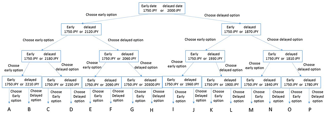
Figure 1. Tree diagram of alternatives. Participants choose whether to receive a lower amount of money at an early date or a higher amount at a later date. After choosing an option, the amount of the delayed option is changed, and the participants face new options. After four iterations, the indifference amount for the delayed option relative to the amount of the early option can be determined. The indifference amount for the delayed option is shown for 16 categories (A, B, …, P). The most impatient preference is A, and the most patient preference is P. The impatience preference ranking is A, B, C, D, E, F, G, H, I, J, K, L, M, N, O, P.
After obtaining the indifference amount of the delayed option relative to the amount of the early option, we calculated the discount factor. In this study, we referred to the discount factors as time preferences. We used a linear utility function: u(x) = x. We assumed the indifference amount of the delayed option relative to the amount of the early option to be xdelayed, and that of the early option to be xearly. Later, we calculated the discount factor δ as , for year t. Because there were two types of dates for the two options, (early date, later date) = (today, 1 month) and (1 month, 2 months), the values of t were 1/12 and 1/12, respectively. We referred to δ as the patience. A high value of δ denoted patience and a low value denoted impatience. Thus, the most impatient preference was A, and the most patient preference was P in Figure 1 because xearly was always 1,750. The impatience preference ranking was A, B, C, D, E, F, G, H, I, J, K, L, M, N, O, P.
There were three choice conditions: an individual condition, a different condition (“for another”), and a group condition. All participants were tested for all three conditions. To control the order effect of the choice conditions, we conducted various combinations of all three conditions. In other words, we conducted six sessions. For the individual condition, participants chose alternatives for themselves; for the “for another” condition, participants chose alternatives for other members of the same group on an individual basis. Here, the chosen option was paid to the other members of their group. The payment mechanism is described in the next paragraph. We failed to analyze the “for another” condition here, because it was described in detail by Truruta et al. [16]3. For the group condition, three participants per group discussed the options using text messages on a computer. As a result, participants could not identify the other group members' gender, visual aspect, race, and so on. We did this to eliminate unobservable effects on decision-making that would result from a face-to-face discussion. Moreover, this enabled us to analyze the text data for each group discussion: for example, the extent of discussion, who expresses an opinion first, and whether persuasion occurs. Subsequently, we investigated our finding that median voter hypothesis was supported (i.e., the median patient member had the greatest impact on group choices). In the group condition, the amount of the reward shown was per person: for example, “Each member is going to receive JPY 1,750 today or JPY 2,000 one month later.” Participants, then, needed to make a group choice through discussion. Hence, the decision rule was unanimity. No time limits were imposed in any of the conditions.
The amount of the reward per person was the same in all three choice conditions. One of the options that the participants chose was selected randomly by the computer, and the selected option was paid to participants. The option that was paid was selected from all group choices a person's group chose under the group condition, all individual choices s/he chose under the individual condition, and all individual choices the other group members (two persons) chose under the “for another” condition. The reward was an Amazon gift card, which was e-mailed to the participant. The advantage of this reward was that we could make the transaction cost the same between the immediate reward and the delayed reward. The average reward was approximately JPY 1,890.
After participants arrived at the laboratory, the instructions were distributed. The instructions4 are included in the Supplementary Material. Participants sat in cubicles and chose the alternatives using a computer. After three choice conditions, we informed participants about the reward they were to be paid, and they completed a post-experimental questionnaire that inquired about their demographic data.
Hypotheses
We formulate two hypotheses. The first hypothesis is based on the multilateral bargaining model. According to this hypothesis, the most patient member in a group has the greatest impact on group choices (multilateral bargaining hypothesis). The second hypothesis is based on the median voter model. According to this hypothesis, the median patient member has the greatest impact on group choices (median voter hypothesis).
Multilateral Bargaining Hypothesis
This subsection describes the multilateral bargaining hypothesis, which is based on the multilateral bargaining model. This hypothesis predicts that the most patient member has the greatest impact on group choices. Our experimental setting is close to multilateral bargaining, in that members of a group negotiate with each other over group choices.
The bilateral bargaining model is well known as a result of Rubinstein's pioneering work [17]. The multilateral bargaining model was developed by Baron and Ferejohn [18] and Banks and Duggan [19] and had been studied mainly in the fields of political science and economics. In the popular model setting of multilateral bargaining [18], a proposer is selected from all members with some probability, who then proposes the allocation of the surplus. Then, the members vote on the proposals (i.e., accept or not accept). Under the majority voting rule, the proposal is implemented and the game ends when the majority of the members vote to accept. Otherwise, the procedure is repeated, including the selection of a proposer [18]. Under the unanimity voting rule, the proposal is implemented and the game ends when all members vote to accept. Otherwise, the procedure is repeated by selecting another proposer [20].
Our experiment differs from these bargaining models, where members decide how to allocate the resource among themselves, because members decide on a common group discount factor (i.e., time preferences) in our experimental setting. Here, we follow Ambrus et al. [6], who studied how individual risk preferences were aggregated in groups and also employed the multilateral bargaining model as a theoretical background. We do so because we also investigate how individual preferences are aggregated in groups. Moreover, applying the multilateral bargaining model is plausible, because people have heterogeneous opinions and make group decisions through discussion in our experimental setting.
The main difference between our hypothesis and that of Ambrus et al. [6] is that we assume heterogeneous individual discount factors, whereas they assume common discount factors among members of a group. Our assumption is closer to how group decisions are made in real-life. Another difference is that we employ the unanimity rule; that is, group members' choices must be the same after the discussion5.
Several theoretical studies based on the multilateral bargaining model assume heterogeneity of individual discount factors and employ the unanimity rule [21–23]. According to these studies, a more patient member receives a higher payoff and has stronger bargaining power. This is because patient members can reject unfavorable proposals more easily than impatient members. The unfavorable option refers to an objective option (i.e., a lower reward). For example, suppose we have a proposer A, a patient member B (δB = 0.9), and an impatient member C (δC = 0.2), when proposer A proposes that A receives 60, B receives 20, and C receives 20 at time t, the patient member B compares 20 to δB (= 0.9) × (the expected allocation of B at t + 1) to decide whether or not to accept the proposal. Similarly, the impatient member C compares 20 to δC (= 0.2) × (the expected allocation of C at t + 1) to decide whether or not to accept the proposal. Here, the impatient member C's expected payoff at t + 1 is likely to be lower than that of the patient member owing to the difference in the discount factors. When B and C's allocations at t + 1 are both 40, the patient member B rejects the proposal at t (20 < 0.9 × 40), but the impatient member C accepts the proposal at t (20 > 0.2 × 40).
We apply this logic to our experimental setting. Thus, the multilateral bargaining hypothesis states that the most patient member has the greatest impact on group choices.
Median Voter Hypothesis
This subsection describes the median voter hypothesis, which is based on the median voter model. This hypothesis predicts that the median patient member has the greatest impact on group choices in our experiment.
The median voter model is well known and is applied in various academic fields [24]. Here, the median voter's choices are selected as the group choices under majority rule if all voters have a single peaked preference [25]. We apply this logic to our experimental setting. Thus, we hypothesize that the median patient member has a significant impact on group choices. According to this hypothesis, we predict that group decisions are conducted under the majority voting rule, not bargaining, even though they can discuss the options freely.
In our experimental setting, the median patient member's final choices are the same as the final group choices when the group members employ the majority voting rule. The explanation is as follows (see Figure 1). First, we consider the situation in which all the members' preferences are different. For example, there are three members of the same group, each of whom prefer a different option (D, E, and F). For the first question (JPY 1,750 at an early date or JPY 2,000 at a later date), all three members select the early option. For the second question (JPY 1,750 at an early date or JPY 2,120 at a later date), the person who likes D the best selects the early option, but the other members select the delayed option. Consequently, the group chooses the delayed option because they employ majority voting. For the third question (JPY 1,750 at an early date or JPY 2,060 at a later date), all three members select the early option. For the fourth question (JPY 1,750 at an early date or JPY 2,090 at a later date), the person who likes F the best selects the delayed option, but the other members select the early option. In this case, the group chooses the early option because they employ majority voting. Therefore, the final group choice is E, which is the same as the median patient member's final choice. The results for the other cases are the same. Second, we consider the situation in which two of the members' final choices are the same. The median patient member always belongs to the majority, because there are three group members. For example, if one member prefers C but the other two prefer D, then the median patient member is the person who prefers D. If one member prefers I but two prefer E, then the median patient member is the person who prefers E. Therefore, the median patient member's final choice is also the final group choice under the majority voting rule, because the median patient member always belongs to the majority. Finally, we consider the situation in which all the members' final choices are the same. Evidently, the median patient member's final choice is the same as the final group choice in this situation.
Consequently, the median voter hypothesis states that the median patient member has the greatest impact on group choices.
Results
Regression Analysis and Post-estimation Analysis
We classify group members into three ranks, as follows. Rank 1, rank 2, and rank 3 represent the order of the discount factor under the individual condition in the same group6. Rank 1 refers to the most patient member (the highest discount factor) in a group, rank 2 refers to the median member (the second highest discount factor), and rank 3 refers to the most impatient member (the third highest discount factor: i.e., the lowest discount factor). If two members in the same group have the same value, we handle it as follows. For example, when the value of member A's discount factor is 0.8, that of member B's discount factor is 0.8, and that of member C's discount factor is 0.7, we set rank 1 and rank 2 to 0.8 and rank 3 to 0.7. If all members of the group have the same value, we set all three rank values to the same value.
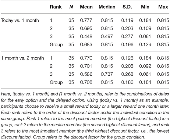
Table 1 shows the descriptive statistics for each rank and the group discount factors for each date. Figure 2 shows the mean discount factors of the (today, 1 month) condition. Figure 3 shows the mean discount factors of the (1 month, 2 months) condition. In both cases, rank 2 seems to be close to the group discount factor.
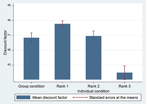
Figure 2. Mean discount factors for the group condition and the individual conditions (Rank 1, Rank 2, and Rank 3). The combination of dates for the early option and the delayed option is (today vs. 1 month). Participants choose to receive a smaller reward today or a larger reward one month later. Each rank refers to the order of the discount factor under the individual condition in the same group. Rank 1 refers to the most patient member (the highest discount factor) in a group, rank 2 refers to the median member (the second highest discount factor), and rank 3 refers to the most impatient member (the third highest discount factor, i.e., the lowest discount factor). Group refers to the discount factor for the group condition.
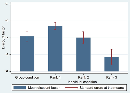
Figure 3. Mean discount factors for the group condition and individual conditions (Rank 1, Rank 2, and Rank 3). The combination of dates for the early option and the delayed option is (1 month vs. 2 months). Participants choose to receive a smaller reward one month later or a larger reward two months later. Each rank refers to the order of the discount factor under the individual condition in the same group. Rank 1 refers to the most patient member (the highest discount factor) in a group, rank 2 refers to the median member (the second highest discount factor), and rank 3 refers to the most impatient member (the third highest discount factor. i.e., the lowest discount factor). Group refers to the discount factor for the group condition.
For a more detailed analysis, we conduct a regression analysis and a post-estimation analysis. These analyses are partially based on the work of Ambrus et al. [6], who also analyze how individual preferences are aggregated at the group level. They investigated risk preferences using a lottery task and selfishness using a gift exchange game. We focus on the model in which the group decision is a linear function of :
where denotes group g's elicited group discount factor, and denotes rank i's elicited individual discount factor in group g. We use to refer to the jth highest discount factor among the individuals in group g (in particular, refers to the highest and refers to the lowest discount factors). We interpret the coefficients (i.e., α1, α2, α3) as the influence of each rank on the group discount factors.
Next, we conduct a post-estimation analysis using our two hypotheses (i.e., the multilateral bargaining hypothesis and the median voter hypothesis): see section Hypotheses. Later, we conducted post-estimation analyses, as follows. First, we test whether the most patient member has the greatest impact on group choices by analyzing whether we can reject α2 = α3 = 0. Subsequently, we test this more strictly by analyzing whether we can reject α2 = α3 = 0 and α1 = 1. If these tests are rejected, we can interpret that the multilateral bargaining hypothesis is rejected. Second, we test whether the median patient member has the greatest impact on group choices by analyzing whether we can rejectα1 = α3 = 0. We also test this more strictly by analyzing whether we can reject α1 = α3 = 0 and α2 = 1. If these tests are rejected, we can interpret that the median voter hypothesis is rejected. Third, we test whether the most impatient member has an impact on group choices. Here, we test whether we can reject α1 = α2 = 0, and we test this more strictly by analyzing whether we can reject α1 = α2 = 0 and α3 = 1. If these tests are rejected, we can interpret from the results that the most impatient member does not have the greatest impact on group choices.
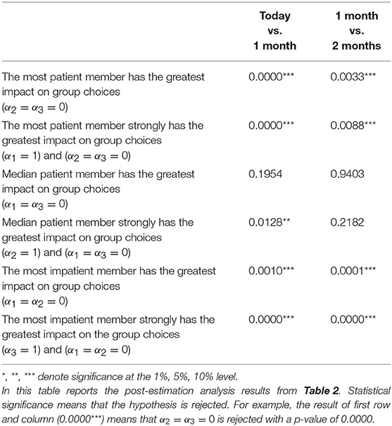
Table 2 shows the results of the regression of the group discount factors on the ordered individual discount factors. The coefficient of the median member's discount factor, α2, is positive and significant for both combinations of dates. Table 3 shows the results of the post-estimation analyses. Here, we reject that “the most patient member has the greatest impact on group choices,” “the most patient member strongly has the greatest impact on group choices,” “the most impatient member has the greatest impact on group choices,” and “the most impatient member strongly has the greatest impact on group choices” for both combinations of dates at the 1% level. We cannot reject “the median patient member has the greatest impact on group choices” and “the median patient member strongly has the greatest impact on group choices” for both combinations of dates at the 1% level. Therefore, we reject the multilateral bargaining hypothesis. In addition, the most impatient member does not have the greatest impact on group choices.
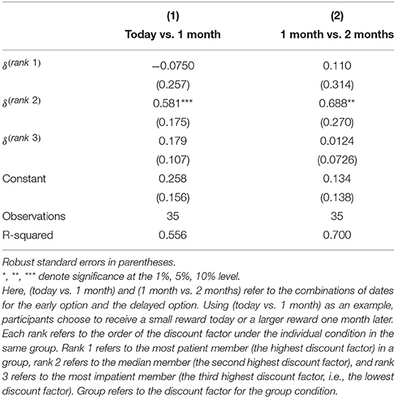
Table 2. Ordinary least squares (OLS) regression of group discount factors on individual discount factors.
Bayesian Analysis
In this subsection, we conduct a Bayesian analysis. As mentioned in the previous subsection, we reject the multilateral bargaining hypothesis. However, rejecting this hypothesis and not rejecting the median voter hypothesis does not guarantee support for the median voter hypothesis. In other words, not rejecting a hypothesis is not the same as supporting the hypothesis [13]. To resolve this problem, we conduct a Bayesian analysis and calculate the Bayes factors. Then, we analyze which hypothesis best fits the experimental data.
We first conduct the following four linear regressions using Bayesian methods and, then, calculate the Bayes factors to judge which hypothesis best fits the experimental data.
where denotes group g's elicited group discount factor, and denotes rank i's elicited individual discount factor in group g. We use to refer to the jth highest discount factor among the individuals in group g (in particular, refers to the highest and refers to the lowest discount factors). Model (2) includes all the members' discount factors as explanatory variables. Model (3) includes only the most patient member's discount factor (i.e., ) as an explanatory variable. Model (4) includes only the median patient member's discount factor (i.e., ) as an explanatory variable. Model (5) includes only the most impatient member's discount factor (i.e., ). If the median voter hypothesis is supported, Model (4) will fit the experimental data better than Models (3) and (5).
To fit a Bayesian parametric model, we need to specify the likelihood function or the distribution of the data and the prior distributions for all model parameters. In Model (2), the Bayesian linear model has five parameters: four regression coefficients (i.e., a constant, δ(rank 1), δ(rank 2), and δ(rank 3)) and the variance of the data. We assume a normal distribution for the dependent variable (i.e., δgroup) and start with a non-informative Jeffreys prior [26] for the parameters. Under the Jeffreys prior, the joint prior distribution of the coefficients and the variance is proportional to the inverse of the variance. In Models (3), (4), and (5), we also assume a normal distribution for the dependent variable (i.e., δgroup) and start with a non-informative Jeffreys prior for the three parameters (i.e., a constant, δ(rank R), and the variance of the data). Here, R is set to 1 in Model (3), 2 in Model (4), and 3 in Model (5).
We can write model (2) as follows:
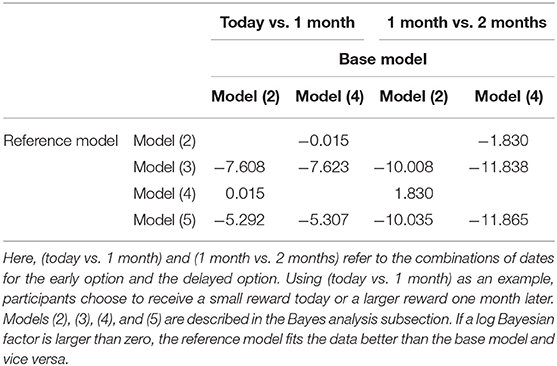
where X is design matrix, and ′, which is a vector of coefficients. In Models (3), (4), and (5), the vector of coefficients is ′, where R is 1 in Model (3), 2 in Model (4), and 3 in Model (5). Next, we calculate the Bayes factors. The Bayes factors compute the relative probabilities of how well each model fits the data, as compared with the base model. We report the log Bayesian factors. If a log Bayesian factor is larger than zero, the reference model fits the data better than the base model and vice versa. We calculate two cases, namely, where the base model is Model (2) and the base model is Model (4). We use the Metropolis-Hastings method. All statistical analyses are performed using STATA 14.0.
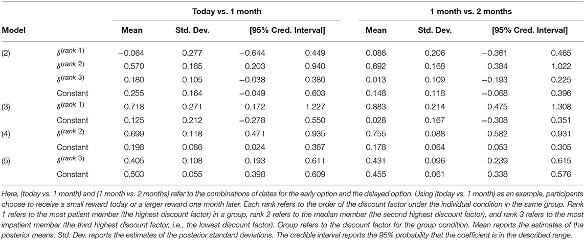
Table 4 shows the results of Bayesian linear regression. The mean reports the estimates of posterior means, which are the means of the marginal posterior distributions of the parameters. Std. Dev. reports the estimates of the posterior standard deviations, which are the standard deviations of the marginal posterior distributions. The credible interval reports the 95% probability that the coefficient is in the described range. In the case of Model (2), only rank 2 has a lower bound of the 95% credible interval that is positive for both combinations of dates for the early option and the delayed option. Therefore, we surmise that rank 2 has a strong influence on group choices. Table 5 shows the log Bayes factors. The first and third columns report the log Bayes factors using Model (2) as a base model. As shown, the value of the log Bayes factor is positive when the reference model is Model (4) for both combinations of dates. Thus, Model (4) fits the data better than Model (2). In other words, the model that includes only the constant and rank 2 is better than the model that includes all of the coefficients. The second and fourth columns report the log Bayes factors using Model (4) as a base model. As shown, the value of the log Bayes factor is negative when the reference model is Model (3) for both combinations of dates. Thus, Model (4) fits the data better than Model (3). In other words, the model that includes the constant and rank 2 is better than the model that includes the constant and rank 1. From these results, we conclude that the median voter hypothesis is supported.
Chat Analysis
We reject the multilateral bargaining model using a regression analysis and a post-estimation analysis in section Regression Analysis and Post-estimation Analysis. In addition, we discover that the median voter hypothesis is supported using a Bayesian analysis in section Bayesian Analysis. In this subsection, we investigate why the median voter hypothesis is supported by analyzing the text data from the group chats.
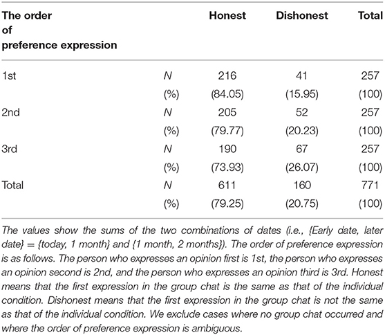
Why does the median patient member have a strong impact on group choices, even though the experimental setting uses the unanimity rule? Here, we focus on the order of preference expression, which we label as follows. The person who expresses an opinion first is 1st, the person who expresses an opinion second is 2nd, and the person who expresses an opinion third is 3rd.
When people express an opinion, this opinion is considered to be closest to their own preferences7. They can discuss whether their opinions differ from those of the other group members. Here, we refer to the choices in the individual condition as a member's own preferences. However, the proportion (the number expressing the opinion closest to own preference) ÷ (the number of all expressions) is only 80%8. In other words, 20% of those expressing an opinion fail to express their individual conditions. Are the proportions of each order of preference expression the same? Table 6 shows the results9. The data in Table 6 show the sum of the two combinations of dates (i.e., {Early date, later date} = {today, 1 month} and {1 month, 2 months}). The proportion of expressions closer to the own preferences declines from 1st to 3rd (i.e., 84.05% in 1st, 79.77% in 2nd, 73.93% in 3rd). The proportions in each order of preference expressions are statistically different [ = 8.0602, p = 0.018]. Multiple comparisons show that the proportion between 1st and 3rd is significantly different (p = 0.014, Bonferroni test), and the proportion between 2nd and 3rd is not significantly different (p = 0.306, Bonferroni test). Thus, those who express their own opinion third fail to express own preferences less often than those who do so first.
Why do people who express 3rd fail to express their own preferences? There are two situations in which “3rd” express their own opinion. First, the first person and the second person express the same opinion. Second, the first person and the second person express different opinions10. If the first person and the second person express the same opinion, the third person's preference differs from theirs, but the third person follows the first two. We call this “dishonesty due to conformity with majority.” For example, 1st chooses the early option and 2nd chooses the early option. Consequently, although 3rd prefers the delayed option, s/he chooses the early option. We call this “conformity with majority.” In the chat data, the total number of dishonest choices by 3rd is 67, as shown in Table 6. Out of these, the number of “dishonesty due to conformity with the majority” is 63. Therefore, there might be a tendency for people to follow the majority, even though they have their own opinions.
We guess that this tendency affected our main findings that the median patient member has the greatest impact on group choices. The “dishonesty due to conformity with majority” works to the median member's advantage, as follows. For example, suppose we have two options, A and B, and three members (x, y, z) who have single-peaked preferences; in this situation, there are four patterns of members' preferences (i.e., {x, y, z} = {A, A, A}, {A, A, B}, {A, B, B}, {B, B, B}). Taking {x, y, z} = {A, A, B} as an example, the number of combinations of the order of preference expressions and own opinions is six (i.e., {1st, 2nd, 3rd} = {Ax, Ay, Bz}, {Ay, Ax, Bz}, {Bz, Ax, Ay}, {Bz, Ay, Ax}, {Ax, Bz, Ay}, and {Ay, Bz, Ax}). Here, Ax indicates that person x chooses option A. It is possible that “dishonesty due to conformity with the majority” occurs when {1st, 2nd, 3rd} = {Ax, Ay, Bz} and {Ay, Ax, Bz}. When the third person z fails to express his/her own opinion B, but instead expresses A to follow the majority, “dishonesty due to conformity with the majority” occurs. Consequently, all three members choose option A. Thus, alternative A (i.e., median person y's preference) is selected as the group choice. We reach the same conclusion for {x, y, z} = {A, B, B}. These cases might increase the significance of the median patient member's effect on group choices.
As discussed above, we guess that the median patient members have a significant impact on group choices, partially because there are many cases of “dishonesty due to conformity with the majority.” Naturally, there might be other reasons why median patient members have an effect on group choices. This is left for future research.
Conclusion
This study investigates how individual intertemporal preferences are aggregated in groups through deliberation, by clarifying who has a significant effect on group choices. We formulated two hypotheses. First, the multilateral bargaining hypothesis is based on the multilateral bargaining model, which predicts that the most patient member in a group has the greatest impact on group choices. Second, the median voter hypothesis is based on the median voter model, which predicts that the median patient member in a group has the greatest impact on group choices. We found that the median patient member has a substantial impact on group choices; that is, the median voter hypothesis is supported. Moreover, we examined the text data from the group chats to investigate why the median voter hypothesis is supported. According to the chat analysis, people who express their own opinion third (i.e., last) tend to follow the majority opinion. This may be one reason for our result (i.e., the median member has the greatest impact on group choices), even though the experimental setting is a free discussion and uses the unanimity rule.
Our results indicate that a median patient member in a group has the greatest impact on group intertemporal choices, even while using a free discussion and the unanimity rule. When workers make investment decisions under these conditions in a meeting, the median patient opinion might be accepted. This finding is surprising because many economists assume that the most patient member has the strongest bargaining power in group choices.
In our experiment, the groups are small and contain an odd number of members (i.e., three). Thus, we cannot generalize our results for an even number of members or for large groups. For an even number of members, we cannot determine whether the more patient median member or the less patient median member has a greater impact. Furthermore, median patient's power may decrease in large groups when compared with small groups. Median member becomes a pivotal member in group decision less often in a large group than in a small group. Thus, the answer to how much impact which median member has in a large group is unknown. Resolving these issues is left to future research.
Data Availability Statement
The raw data supporting the conclusions of this manuscript will be made available by the authors, without undue reservation, to any qualified researcher.
Author Contributions
MT developed the study concept and the experimental paradigm and conducted the experiment. MT performed the data analysis and interpretation under the supervision of KI. MT and KI drafted the manuscript. Both authors contributed to the discussion section of the manuscript and approved the work for publication.
Funding
This work was supported by the Japan Society for the Promotion of Science Grant-in-Aid for Scientific Research JP17H04780 JP 15K13007 for KI and 15H05728 for Yoshiyasu Ono, the Top-Setting Program to Advance Cutting-Edge Humanities and Social Sciences Research, and the Joint Usage/Research Center at ISER, Osaka University.
Conflict of Interest Statement
The authors declare that the research was conducted in the absence of any commercial or financial relationships that could be construed as a potential conflict of interest.
Acknowledgments
We thank the faculty and staff of the Center for Behavioral Economics at ISER, Osaka University, who kindly allowed us to use their laboratory resources.
Supplementary Material
The Supplementary Material for this article can be found online at: https://www.frontiersin.org/articles/10.3389/fams.2018.00043/full#supplementary-material
Footnotes
1. ^Bixter et al. [1] also studied group and individual time preferences. They investigated whether individual choices after group decisions are affected by group agreement.
2. ^Of course, there are cases where all the members' individual discount factors are same or two of the three members' individual discount factors are same. We explain how we handled these cases in section Regression Analysis and Post Estimation (Regression analysis and post estimation).
3. ^We do not include the “for another” condition in our analysis because we are not interested in this category in this study. See Tsuruta [16] for a discussion of this condition. Thus, we analyze only the group and individual conditions.
4. ^The instruction is written in Japanese.
5. ^In their experimental setting, Ambrus et al. [6] employed the unanimity rule, as we did. However, they built their hypothesis using both the unanimity rule and the majority rule.
6. ^We explain how to calculate discount factor (i.e., time preferences) in section Methods.
7. ^For example, the person who prefers D in Figure 1 is considered to choose the early option for the first question (JPY 1,750 at an early date or JPY 2,000 at a later date).
8. ^We check whether people's opinions are the same as those of the individual conditions. We do not count opinions that change during the discussion and count only the first expression in each question. There is one expression per person in each question. As mentioned in the Method section, there are four expressions for one combination of dates for the early option and the delayed option, there are two combinations of dates (i.e., {today, 1 month} and {1 month, 2 months}), and there are 105 participants. Therefore, the number of all first expressions is 840 (4 × 2 × 105 = 840). Out of these, the number of first expressions not close to the own preferences is 168. Therefore, (the number choosing an option NOT closer to own preference) ÷ (the number of all expressions) = 168/840 = 0.2.
9. ^We exclude cases where no chat occurred or where the order of preference expression is ambiguous in Table 6. Therefore, the final sample is 771.
10. ^As mentioned in the Method section, participants always face a choice between two options.
References
1. Bixter MT, Trimber EM, Luhmann CC. Are intertemporal preferences contagious? Evidence from collaborative decision making. Mem Cogn. (2017) 45:837. doi: 10.3758/s13421-017-0698-z
2. Yang X, Carlsson F. Influence and choice shifts in households: an experimental investigation. J Econ Psychol. (2016) 53:54–66. doi: 10.1016/j.joep.2015.11.002
3. Carlsson F, He H, Martinsson P, Qin P, Sutter M. Household decision making in rural china: Using experiments to estimate the influences of spouses. J Econ Behav Organ. (2012) 84:525–36. doi: 10.1016/j.jebo.2012.08.010
4. Charness G, Sutter M. Groups make better self-interested decisions. J Econ Perspect. (2012) 26:157–76. doi: 10.1257/jep.26.3.157
5. He H, Villeval MC. Are group members less inequality averse than individual decision makers? J Econ Behav Organ. (2017) 138:111–24. doi: 10.1016/j.jebo.2017.04.004
6. Ambrus A, Greiner B, Pathak P. How individual preferences are aggregated in groups: an experimental study. J Public Econ. (2015) 129:1–13. doi: 10.1016/j.jpubeco.2015.05.008
7. Shupp RS, Williams AW. Risk preference differentials of small groups and individuals. Econ J. (2008) 18:258–83. doi: 10.1111/j.1468-0297.2007.02112.x
8. Harrison GW, Lau MI, Rutström EE, Tarazona-Gómez M. Preferences over social risk. Oxford Econ Pap. (2013) 65:25–46. doi: 10.1093/oep/gps021
9. Baker RJ II, Laury SK, Williams AW. Comparing small-group and individual behavior in lottery-choice experiments. South Econ J. (2008) 75:367–382.
10. Bone J, Hey J, Suckling J. Are groups more (or less) consistent than individuals? J Risk Uncertain. (1999) 18:63–81. doi: 10.1023/A:1007764411446
11. Masclet D, Colombier N, Denant-Boemont L, Lohéac Y. Group and individual risk preferences: a lottery-choice experiment with self-employed and salaried workers. J Econ Behav Organ. (2009) 70:470–84. doi: 10.1016/j.jebo.2007.11.002
12. Bateman I, Munro A. An experiment on risky choice amongst households. Econ J. (2005) 115:C176–89. doi: 10.1111/j.0013-0133.2005.00986.x
13. Gallistel CR. The importance of proving the null. Psychol Rev. (2009) 116:439–453. doi: 10.1037/a0015251
14. Fischbacher U. z-Tree: Zurich toolbox for ready-made economic experiments. Exp Econ. (2007) 10:171. doi: 10.1007/s10683-006-9159-4
15. Read D. Is time-discounting hyperbolic or subadditive? J Risk Uncertain. (2001) 23:5. doi: 10.1023/A:1011198414683
16. Truruta M. Group and individual Time Preferences in Laboratory Experiments. In: Discussion Papers in Economics and Business (Osaka University) (2016) 16:11.
17. Rubinstein A. Perfect Equilibrium in a Bargaining Model. Econometrica (1982) 50:1. doi: 10.2307/1912531
18. Baron D, Ferejohn J. Bargaining in legislatures. Am Polit Sci Rev. (1989) 83:1181. doi: 10.2307/1961664
19. Banks J, Duggan J. A bargaining model of collective choice. Am Polit Sci Rev. (2000) 94:73–88. doi: 10.2307/2586381
20. Merlo A, Wilson C. Efficient delays in a stochastic model of bargaining. Econ Theory (1998) 11:39. doi: 10.1007/s001990050177
21. Cardona D, Rubí-Barceló A. Time-preference heterogeneity and multiplicity of Equilibria in two-group bargaining. Games (2016) 7:2. doi: 10.3390/g7020012
22. Kawamori T. Players' Patience and Equilibrium Payoffs in the Baron–Ferejohn Model. Econ Bull. (2005) 3:1–5.
23. Yildirim H. Proposal power and majority rule in multilateral bargaining with costly recognition. J Econ Theory (2007) 136:167–96. doi: 10.1016/j.jet.2006.07.008
24. Congleton RD. the median voter model. In: Rowley CK, Schneider F, editors. The Encyclopedia of Public Choice. Boston, MA: Springer (2004), p. 707–12. doi: 10.1007/978-0-306-47828-4_142
25. Black D. On the rationale of group decision-making. J Polit Econ. (1948) 56:23–34. doi: 10.1086/256633
Keywords: intertemporal choice, impatience, group decision-making, multilateral bargaining, median voter model, laboratory experiment, chatting, conformity with majority
Citation: Tsuruta M and Inukai K (2018) How Are Individual Time Preferences Aggregated in Groups? A Laboratory Experiment on Intertemporal Group Decision-Making. Front. Appl. Math. Stat. 4:43. doi: 10.3389/fams.2018.00043
Received: 20 April 2018; Accepted: 23 August 2018;
Published: 02 October 2018.
Edited by:
Taiki Takahashi, Hokkaido University, JapanReviewed by:
Barret Pengyuan Shao, Independent Researcher, Washington, DC, United StatesFuat Balci, Koç University, Turkey
Naoshi Tsuchida, Bank of Japan, Japan
Copyright © 2018 Tsuruta and Inukai. This is an open-access article distributed under the terms of the Creative Commons Attribution License (CC BY). The use, distribution or reproduction in other forums is permitted, provided the original author(s) and the copyright owner(s) are credited and that the original publication in this journal is cited, in accordance with accepted academic practice. No use, distribution or reproduction is permitted which does not comply with these terms.
*Correspondence: Manami Tsuruta, dHN1cnV0YWJvbm9AZ21haWwuY29t
 Manami Tsuruta
 Keigo Inukai