Assessing future changes in hydroclimatic processes in the Metropolitan Region of Belo Horizonte, Brazil, with the expanded Bluecat framework

General circulation models (GCM) have comprised ubiquitous tools for supporting water resources planning and decision-making under changing climate conditions. However, GCMs are often highly biased, which may limit their utilization for representing future trajectories of the hydroclimatic processes of interest. In addition, assessing the predictive uncertainty of climate models, which is paramount for simulation purposes, is not straightforward. For tackling these problems, in this paper we resort to the expanded Bluecat framework, which utilizes empirical conditional distributions for providing a complete stochastic representation of GCM outputs simultaneously to bias correction. The stochastic model was employed for assessing future trajectories of monthly rainfall and temperatures, under three Shared Socioeconomic Pathways, namely, SSP1-2.6, SSP2-4.5, and SSP5-8.5, in the Metropolitan Region of Belo Horizonte, Brazil. Our results indicated that e-Bluecat properly corrected bias for both variables and provided coverage probabilities close to the theoretical ones. Nonetheless, the resulting uncertainty, as materialized by confidence intervals, was deemed too large, which implicitly reflects the inability of the GCMs in describing the observed processes. In addition, in median terms, the bias-corrected estimates suggest considerably smaller increases in temperatures (~1°C), as compared to the climate models (up to 5°C), in all future scenarios. These findings suggest that deterministic outputs of GCMs may present limitations in effectively informing adaptation strategies, necessitating complementary approaches. Moreover, in view of the large uncertainty levels for the projected climate dynamics, simulating critical trajectories from the stochastic model is paramount for optimizing the allocation of financial resources over time in the study area.

1 Introduction

Anthropogenic climate change (ACC) has become a matter of paramount importance for both social and environmental sustainability (Sarker, 2022; Gabric, 2023). In effect, according to the Intergovernmental Panel on Climate Change (IPCC), ACC is expected to alter the patterns of variability of hydroclimatic processes due to global warming (Sarker, 2022), which has led to growing concerns on the intensification of extreme meteorological and hydrological events (IPCC, 2023; Malede et al., 2024). In particular, many regions of the world may experience prolonged dry spells and more severe drought events, which would pose significant challenges for the management of water resources systems (Malede et al., 2024; Tegegne and Melesse, 2020). As a result, recent literature has focused on investigating future changes in the spatiotemporal distribution of water (mainly its occurrence as precipitation) and in temperatures—arguably the main drivers of meteorological droughts—as a response to ACC.

The future dynamics of hydroclimatic processes is frequently inferred from climate models [or Global Circulation Models (GCM)], which are forced under distinct scenarios of greenhouse gases concentrations (GGC) and economic development intended to translate the impacts of anthropogenic activities on the global climate patterns (Brêda et al., 2020; IPCC, 2023). Information from climate models has underpinned most of the discussion on potential effects and adaptation strategies to climate change (Chiew et al., 2022). However, such models are rarely able to capture the actual evolution of climate-related variables, irrespective of the considered emission scenario and the initial/boundary conditions (Muerth et al., 2013; Koutsoyiannis and Montanari, 2022b). In fact, incomplete knowledge on natural systems—and therefore their imperfect representation in model structures—may introduce high levels of bias to model predictions (Rajulapati and Papalexiou, 2023). As climate models' components are frequently nonlinear, this bias may be greatly amplified as the prediction errors propagate over time (e.g., Koutsoyiannis, 2010; Montanari and Koutsoyiannis, 2014), possibly leading to physically unrealistic trajectories for the modeled processes (Chiew et al., 2022; Tegegne et al., 2019; Tegegne and Melesse, 2020). Furthermore, climate models depend on a very large number of (interrelated) parameters, which may hinder the quantification of the epistemic and the predictive uncertainties (Bastola et al., 2011; Wang et al., 2020). Consequently, climate models raw outputs may not be useful for decision-making in many situations (Koutsoyiannis and Montanari, 2022b), despite their widespread utilization in water sciences and other fields.

For tackling these problems, several techniques for bias correction have been explored in previous research. These techniques may simply involve the scaling of low order moments, such as the mean and the variance, or the matching of the entire distributions under variants of a general class of methods termed quantile mapping—which may encompass parametric, semiparametric or machine learning models (Bastola et al., 2011; Rajulapati and Papalexiou, 2023; Sa'adi et al., 2024; Wang et al., 2020). To different extents, these approaches may remove systematic bias and improve the information that stems from raw climate model outputs. However, they are not effective for summarizing the inherent variability of the observed realizations of the hydroclimatic processes of interest with respect to the climate model outputs (i.e., the conditional distributions), which, in turn, limits their utilization for simulation purposes (Koutsoyiannis and Montanari, 2022a,b).

Based on this gap, Koutsoyiannis and Montanari (2022a,b) have recently discussed a simple modeling framework, termed expanded “Brisk local uncertainty estimator for generic simulations and predictions” (hereafter denoted e-Bluecat for simplicity), that simultaneously corrects bias and derives the empirical distribution functions of the observations conditioned on the raw climate model outputs. This framework provides a complete stochastic description of climate projections, which is interesting for tracking critical trajectories of processes that are not described by the bias-corrected deterministic model. Also, it may provide multiple inputs for hydrological modeling, which are frequently required for water resources management and risk assessment. e-Bluecat was applied for bias correction of precipitation and temperature over the entire territory of Italy, which is a relatively large area with no prominent seasonal climate characteristics—climate models are usually more accurate in these cases (Koutsoyiannis and Montanari, 2022b). Results demonstrated that e-Bluecat was able to remove bias and reproduce “observed trends” in distinct ranges of the hydroclimatic variables. Furthermore, it provided appropriate coverage probabilities throughout the historical period of simulation.

In this paper, we further explore the e-Bluecat framework for simulating historical and future dynamics of precipitation and temperature in the Metropolitan Region of Belo Horizonte (MRBH). Given the region's reliance on reservoirs for water supply, the study's findings may contribute to the understanding of potential vulnerabilities to increases in temperature and long dry spells. The main distinction of this study, with respect to the paper of Koutsoyiannis and Montanari (2022b), is that the MRBH is a somewhat small area (~10, 000 km²), with marked seasonality in the rainfall regime. In effect, it has been widely acknowledged that, for fine spatial scales, uncertainty of climate models may be too high because of downscaling (Bastola et al., 2011; Wang et al., 2020). Moreover, assessing e-Bluecat in regions with complex climate regimes and very distinct precipitation generation mechanisms, such as the MRBH, is yet to be tackled. Hence, this application may provide additional insights on the performance of e-Bluecat in more challenging conditions for bias-correction and uncertainty estimation. The remainder of this paper is organized as follows. In Section 2, the study area is presented and details on the expanded Bluecat framework are provided. Section 3 describes the main results of the study along with a comprehensive discussion of advantages and limitations of the proposed approach. Finally, In Section 4, the concluding remarks and envisaged research development are addressed.

2 Materials and methods

2.1 Study area and data

The MRBH is located in the Brazilian state of Minas Gerais, in the southeastern region of the country. The MRBH is a densely populated area, which encompasses 26 municipalities and covers 9, 441km² (Figure 1). A diversity of economic activities, which have required increasing amounts of water, are developed in the region—these include mining, agriculture, industry and services. Water supply in the MRBH strongly relies on three reservoirs: Rio Manso, Serra Azul, and Vargem das Flores. This dependence makes the region highly vulnerable to droughts, as demonstrated by some severe and extreme events in the last decade (Rodrigues et al., 2019). In this sense, stochastic simulation of rainfall and temperature might comprise an effective approach to assess critical situations, such as future drought scenarios, in the study area. This could be helpful for decision makers in developing strategies for adaptation to the effects of climate change in water availability and for increasing resilience to rainfall shortages in the MRBH.

Figure 1

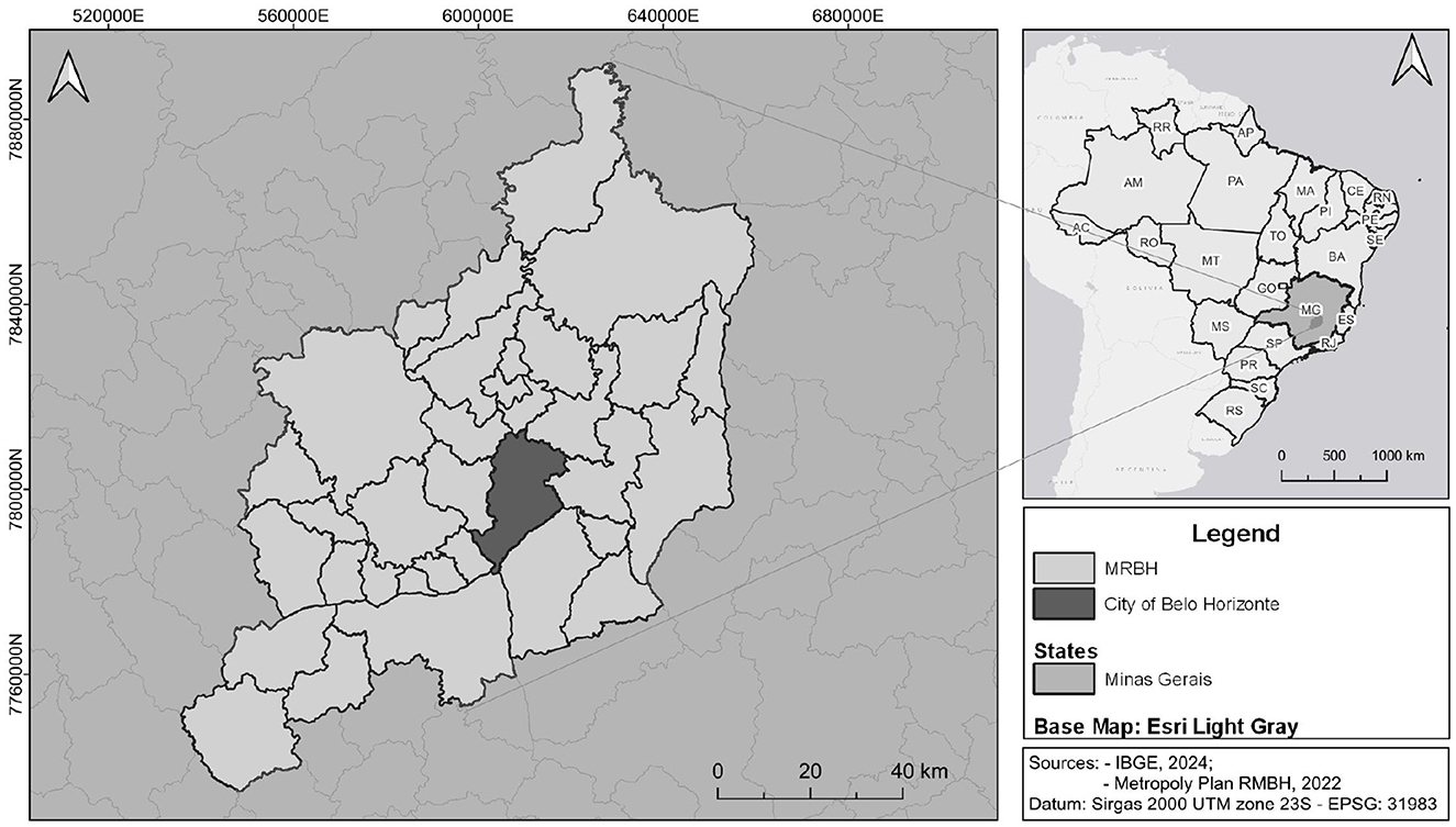
Figure 1. Location of MRBH and highlighting the city of Belo Horizonte.

Climate in the MRBH is predominantly tropical and presents a marked seasonality, with a wet season spanning from October to March, and a dry counterpart from April to September. The average rainfall amounts vary between 200mm to 350mm in the wet months—which amount for ~85% of the mean annual rainfall, and from 0 to 20mm during the dry season. Average monthly temperatures, in turn, range from 22 to 24°C in the wet season, and 18–20° in the dry months. Finally, annual evaporative demands amount ~1, 000mm.

In this paper, the monthly time scale is utilized for assessing the descriptive and predictive abilities of e-Bluecat—despite not being suitable for modeling extreme flooding events, this resolution is appropriate for dealing with droughts, which have become a major concern in the Brazilian southeastern region since the extreme event that occurred in 2013/2014 (Rodrigues et al., 2019)—rainfall amounts were 40% below average during this period. Monthly rainfall data, from 1961 to 2021, were obtained from the digital platform of the Brazilian Agency of Water and Sanitation (ANA, 2024) and from the National Meteorology Institute (INMET) database (INMET, 2024). The selected rainfall gauging stations are shown in Figure 2. Among these, only stations 1943023, 1944004, and 83587 have no missing data during the period-of-record. For the remaining ones, the daily missing values were filled through multiple linear regression using the R package “hyfo” (Xu, 2015). Rainfall data were spatialized over the study area with the Thiessen polygons method.

Figure 2

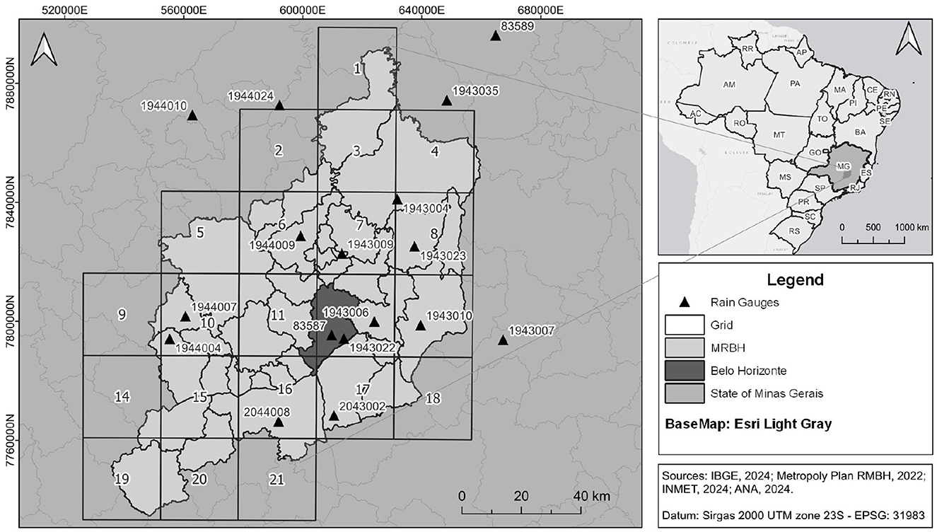
Figure 2. Spatial distribution of grids and rain gauges applied.

As for temperature, we utilized the gridded reanalysis dataset from the European Center for Medium-Range Weather Forecasts (ECMWF) Re-Analysis (ERA5) (Hersbach et al., 2020), in view of the limited availability of climatological stations in the region. Average monthly temperature data were obtained as a raster matrix layer by using the “download_ERA()” tool from R Studio (Kusch and Davy, 2022). Again, the period-of-record for calibrating and validating e-Bluecat ranged from 1961 to 2021.

Finally, gridded estimates for the historical and projection periods, with spatial resolution of 27.8km×27.8km, were obtained, at the daily time scale, from the NASA Earth Exchange Global Daily Downscaled Projections, derived from the Coupled Model Intercomparison Project Phase 6 GCMs (NEX-GDDP-CMIP6) (Rama Nemani, 2021; Thrasher et al., 2022). This dataset is obtained by applying the Bias-Correction Spatial Disaggregation method discussed in Wood et al. (2004) to the Global Meteorological Forcing Dataset (GMFD), at the 0.25° resolution. The downscaling procedure, which is intended to provide more detailed information on the processes at the regional scale, is as follows. First, the GMFD is resampled to the resolution of the original GCM. Then, a quantile mapping procedure is utilized for “scaling” the raw GCM outputs according to the resampled observations (Xu and Wang, 2019). Finally, the corrected GCM output is interpolated, based on the “scaling factor” estimated in the previous step, at resolution of the original observational dataset (Thrasher et al., 2022).

Information for 35 GCMs is available in NEX-GDDP-CMIP6 from 1950-01-01 to 2100-12-31 (Thrasher et al., 2022) for the climate change scenarios utilized in this study, namely, SSP1-2.6, which is an optimistic scenario in which the emissions steadily decline from 2020 to 2100, when it reaches zero; SSP2-4.5, which is a baseline scenario in which emissions increase up to 2040 and then decline; and SSP5-8.5, which is a pessimistic scenario in which emissions steadily increase until 2100 (IPCC, 2023). For averaging the hydroclimatic variables across the study region, 21 grids were defined, as shown in Figure 2—each grid has a “weight” proportional to the overlapping areas among the pixels and the boundaries of the MRBH. After spatial averaging, we build the “ensemble” by simply computing the arithmetic means of the 35 GCM estimates at each month, as usual (e.g., Koutsoyiannis and Montanari, 2022b). We note that more effective approaches for building the ensemble have been reported in recent literature (e.g., Sa'adi et al., 2024 and references therein), but unless some of the GCM components are able to reproduce higher order moments of the observed processes, these techniques are not expected to improve the performance of e-Bluecat.

Figure 3 depicts the annual rainfall amounts, as obtained from the GCM ensemble in the MRBH—here, we consider both the historical (1950–2014) and the projection (2015–2100) periods, the latter for scenarios SSP1-2.6, SSP2-4.5 and SSP5-8.5. One may notice that the SSP1-2.6 scenario suggests a positive “jump” in the average rainfall amounts from 2015 to 2100, as opposed to the remaining ones, for which slight to moderate reductions in such variable are expected. Moreover, no noticeable trends for precipitation are observed for any of the scenarios during the projection period. Similarly, Figure 4 illustrates the trajectories for annual mean temperatures, under the same scenarios. For this variable, however, upward trends are already perceived during the historical period (starting in the 1990s) and the three scenarios indicate increases for the projection counterpart. The SSP1-2.6 scenario presents an upward trend until the mid-2050s, but this trend apparently vanishes from point onwards. In the SSP2-4.5 scenario, a more pronounced increase in annual temperature is observed between 2015 and 2055, and then a less steep rise stems up to 2100. For the SSP5-8.5 scenario projections, a very sharp rise throughout the period from 2015 to 2100 is verified.

Figure 3

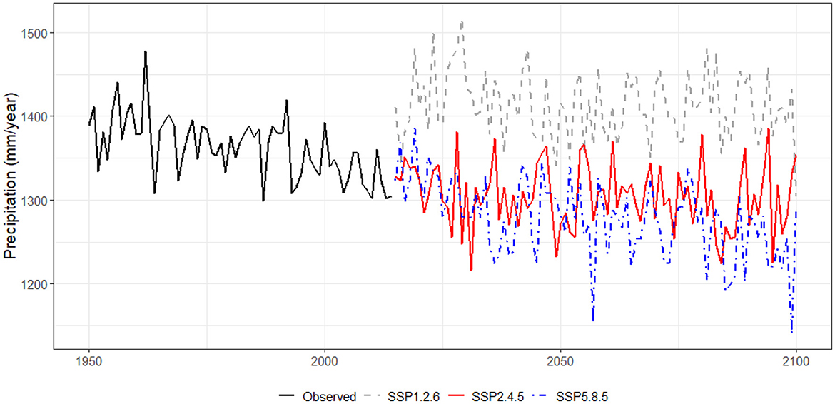
Figure 3. Trajectories for annual mean rainfall amounts under scenarios SSP1-2.6, SSP2-4.5, and SSP5-8.5.

Figure 4

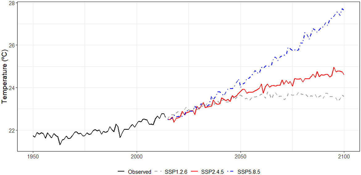
Figure 4. Trajectories for annual mean temperatures under scenarios SSP1-2.6, SSP2-4.5, and SSP5-8.5.

2.2 The expanded Bluecat (e-Bluecat) framework

For deriving the stochastic model, let us assume that q comprises a hydroclimatic stochastic process (e.g., rainfall or temperature), with distribution function F_q(q) and probability density function f_q(q). Also, let Q be an estimator for process q (e.g., climate model outputs), with distribution function F_Q(Q) and probability density function f_Q(Q) (note that, following Koutsoyiannis and Montanari, 2022a,b, underlined symbols comprise stochastic variables and processes, whereas non-underlined ones are related to regular counterparts). Finally, suppose that q and Q are sampled concurrently at discrete times t. The reasoning behind eBlucat is converting the deterministic climate model into a stochastic one through the following conditional distribution

$\begin{array}{ll}{F}_{q|Q}\left(q|Q\right)={\displaystyle {\int }_{-\infty }^q{f}_{q|Q}}\left(q|Q\right)dq=\mathrm{Pr}\left\{\underset{\_}{q}<q|\underset{\_}{Q}=Q\right\}& (1)\end{array}$

which should obey the obvious constraints ${\int }_{-\infty }^{\infty }{f}_{q|Q}(q|Q)dq=1$, ${\int }_0^1{f}_{q|Q}(q|F_Q^{-1}(z))dz=f_q(q)$ and ${\int }_0^1{F}_{q|Q}(q|F_Q^{-1}(z))dz=F_q(q)$ (by definition, z = F_Q(Q) and dz = f_Q(Q)dQ). Equation 1 inherently acknowledges the inability of the climate model in fully representing the observed realizations of q, provided that the distribution is not degenerated. In effect, the variance of the conditional distribution accounts for the proportion of the observed variability that cannot be accounted for by the climate model. Hence, if the climate model provides a suitable representation of the observed process, the variance should be small. Otherwise, the dispersion around q becomes large.

Although some parametric form may be specified for the marginal distribution functions of q and Q, such measures may be also approximated by empirical plotting positions, which makes calculations easier. Here, following (Koutsoyiannis and Montanari, 2022b), we utilize the unbiased estimator of the quantity −ln(F/(1−F)), termed excess return period (in log scale), for this purpose, but other plotting positions could be used as well. The empirical cumulative frequencies are then expressed as

$\begin{array}{ll}{F}_q\left(q_{(i,N)}\right)\approx \frac{i-0.439}{N+0.123}& (2)\end{array}$

$\begin{array}{ll}{F}_Q\left(Q_{(j,N)}\right)\approx \frac{j-0.439}{N+0.123}& (3)\end{array}$

in which q_(i:N) and Q_(j:N) are, respectively, the ith and jth order statistics of the observed samples of q and Q, both of which with size N.

On the other hand, deriving the conditional distribution F_q|Q(q|Q) solely based on data is not straightforward. In fact, both q and Q are continuous random variables, for which each realization is not expected to be observed more than once in a particular time series. Hence, it would not be feasible to empirically estimate the distribution for a given Q, as only the concurrent observation of q (at time τ) would be included in the sample (Koutsoyiannis and Montanari, 2022a). For circumventing this problem with no strong assumptions on the functional form of the joint distribution F_{q, Q}(q, Q) (e.g., copulas or multivariate distributions), Koutsoyiannis and Montanari (2022a) suggested building the q-sample from a set of neighbors of each Q. Formally

$\begin{array}{ll}\begin{array}{r}\hfill F_{q|Q}\left(q|Q\right)\approx \text{Pr}\left\{\underset{\_}{q}<q|Q-\Delta Q\le \underset{\_}{Q}\le Q+\Delta Q\right\}\\ \hfill =\text{Pr}\left\{\underset{\_}{q}<q|F_Q\left(Q\right)-\Delta F\le F_Q\left(Q\right)\le F_Q\left(Q\right)+\Delta F\right\}\end{array}& (4)\end{array}$

in which ΔF (or ΔQ) should allow aggregating a suitable number of realizations of q for reliably estimating the conditional distribution and, at the same time, be as small as possible so that F_Q(Q)±ΔF does not deviate much from F_Q(Q). A simple alternative for defining the increment in the non-exceedance probability is setting ΔF = m/N, in which m denotes the number of Q-neighbors to be included in the sample—this results in 2m+1 values of q for each Q. The empirical conditional distribution may thus be written as

$\begin{array}{ll}{F}_{q(i:2m+1)|Q}\left(q|Q\right)=\frac{i-0.439}{2m+1+0.123}& (5)\end{array}$

This approach, however, renders estimating the empirical distribution for Q<Q_(m+1:N) and Q>Q_(N−m:N) unfeasible. For these cases, one may specify parameters c_l≠1 and c_u≠1 so that Q_(m+1:N) ≤ c_lQ_l and Q_(N−m:N)≥c_uQ_u, in which l refers to lower bound and u refers to upper bound. This allows building “synthetic” samples of q for the lower and upper order statistics of Q, and even extrapolate for unobserved values of the hydroclimatic process of interest. The conditional distribution functions for the extrapolation ranges may be approximated as

$\begin{array}{ll}{F}_{q|Q}\left(q|Q\right)\approx F_{q|Q}\left[q+a_l\left(1-\frac{1}{c_l}\right)c_{l}Q|c_{l}Q\right],forQ<Q_{(m+1:N)}& (6)\end{array}$

and

$\begin{array}{r}{F}_{q|Q}\left(q|Q\right)\approx F_{q|Q}\left[q+a_u\left(1-\frac{1}{c_u}\right)c_{u}Q|c_{u}Q\right],for\\ Q>Q_{(N-m:N)}& (7)\end{array}$

in which a_. denotes the slopes of a linear regression model for the lower (a_l) and upper (a_u) portions of the scatterplot between q and Q (Figure 5). One may notice that extrapolation of the real process is a function of the estimates of the climate model, which, depending on the climate change scenario, may suggest increases (or reductions) of the hydroclimatic processes well beyond (or below) the observed ranges (e.g., Figures 3, 4). Hence, for building samples with size 2m+1 for the entire projection period—usually 2015 to 2100–, one may assume that c_lQ_l = Q_(m+1:N) and c_uQ_u = Q_(N−m:N), in which Q_l and Q_u are, respectively, the smallest and the largest values of Q in the extrapolation range; this allows estimating c_l and c_u.

Figure 5

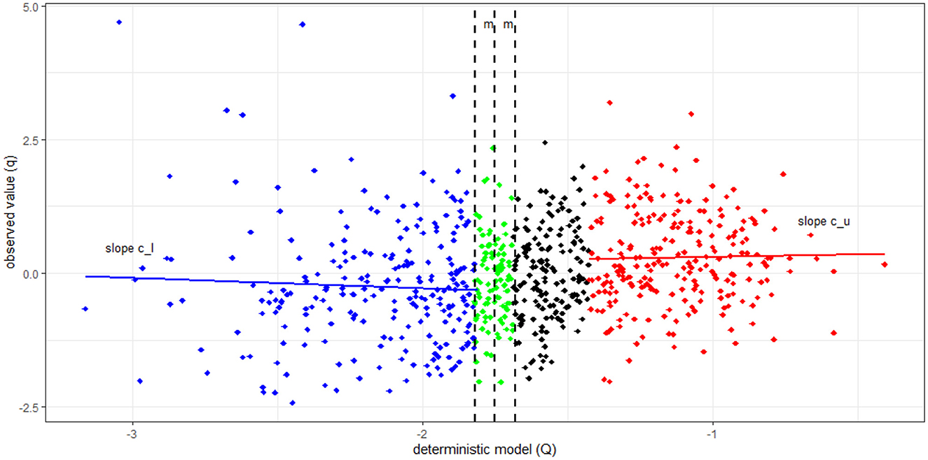
Figure 5. Scatterplot between q and Q (distance between vertical dashed lines is given by 2m + 1).

The approximations in Equations 6, 7 are precise for Gaussian processes; for non-Gaussian counterparts, we utilize the following transformation (Koutsoyiannis and Montanari, 2022a)

$\begin{array}{ll}{q}^{\prime }=\alpha ln\left(1+\frac{q}{\alpha }\right)& (8)\end{array}$

in which α is a parameter estimated by minimizing the quadratic differences among the empirical frequencies, as obtained by the Blom plotting position (which is unbiased for quantiles of the Gaussian distribution; see Naghettini, 2017), and the theoretical probabilities derived from the fitted Gaussian model after the transformation. We note that Equation 8 maps to the logarithmic function as α → 0 and to the identity function as α → ∞. Besides, the transformation maps zero to itself (Koutsoyiannis and Montanari, 2022a).

For bypassing the effects of seasonality in model identification (e.g., cyclostationarity), we linearly transform the original variables by subtracting the long-term monthly averages prior to the application of e-Bluecat. This preserves as much information as possible, in terms of Q-neighbors, for building the conditional empirical conditional distributions (Koutsoyiannis and Montanari, 2022b). Figure 6 provides an example of such distribution, for Q = 1.75 and m = 50 after removing seasonal effects. The e-Bluecat framework is summarized in Figure 7.

Figure 6

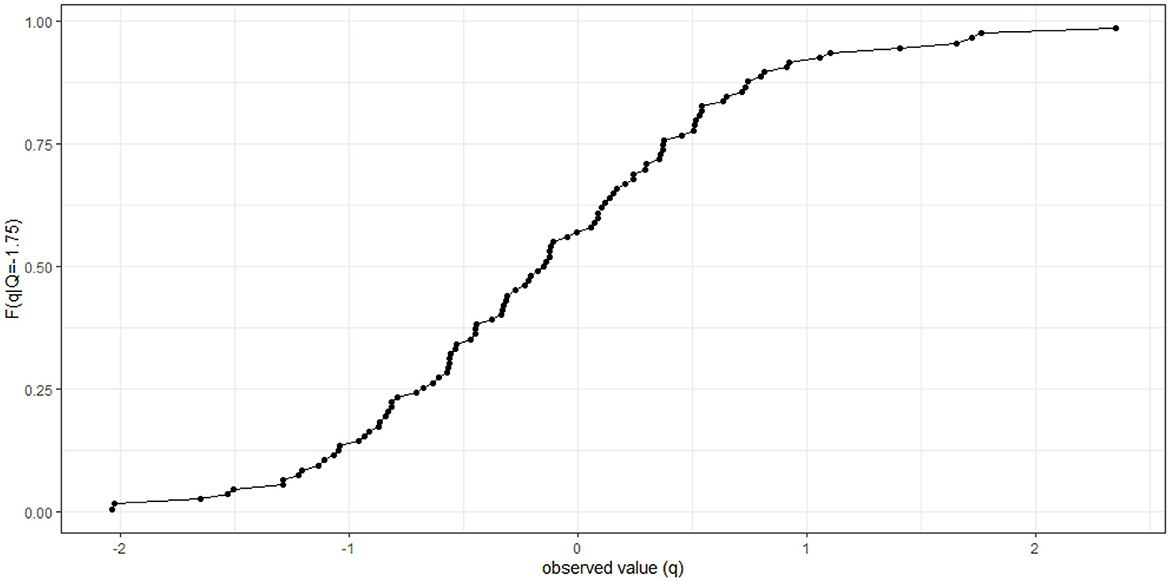
Figure 6. Conditional empirical conditional distribution, for Q = 1.75 and m = 50 after removing seasonal effects.

Figure 7

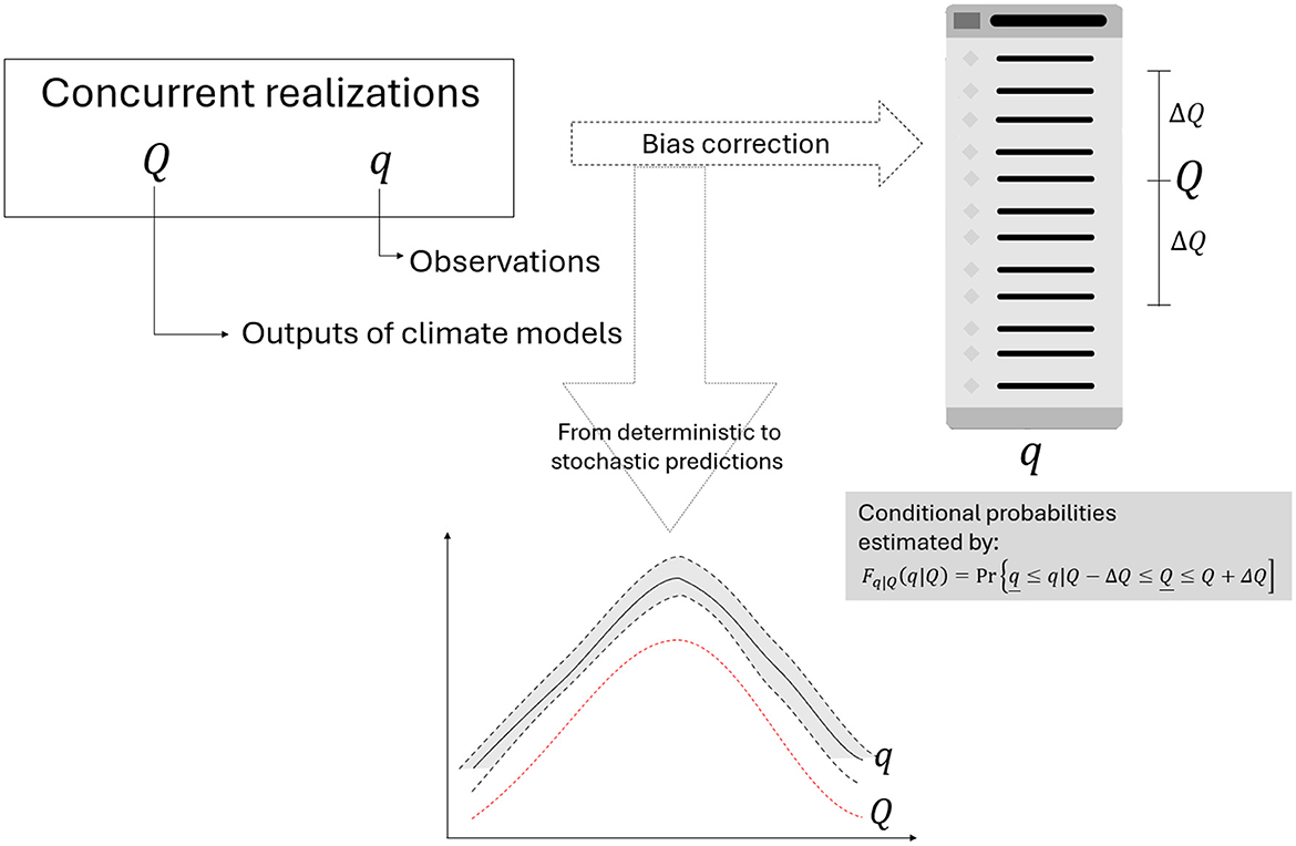
Figure 7. Flowcharf of e-Bluecat.

As concurrent observations of q and Q are available from 1961 to 2021, we have split the sample for performing an ad hoc validation of the model: the first 50 years of the period-of-record were utilized for deriving the conditional distributions in Equation 1, whereas the subsequent period would provide testing conditions (i.e., prediction). As e-Bluecat is fully stochastic, we assess its predictive abilities by comparing the theoretical coverage probability—here defined as 90%-, and the actual ones. Moreover, for obtaining further insights on the effects of each climate change scenario on the conditional distributions, i.e., the prediction uncertainty, we also estimate the average width of the 90% confidence intervals; these should be wider for worst performing climate models (note that the confidence intervals are built with respect to the observed values and not the climate model estimates).

As compared to other well-established bias-correction techniques (see, for instance, Dinh and Aires, 2023, and references therein), e-Bluecat provides a formal probabilistic account of the processes' variability with respect to the observations, not GCM estimates—previous research has indicated that even sophisticated deterministic bias-correction techniques may be unable to reproduce the variances of the observed processes (Maraun et al., 2017). Moreover, the conditional representation of the processes, to a great extent, avoids implausible changes in the climate signals after deterministic bias-correction (Maurer and Pierce, 2014; Maraun, 2016; Maraun et al., 2017), which could result in ill-posed adaptation strategies for water resources management. Finally, as e-Bluecat may be applied for simulation (Koutsoyiannis and Montanari, 2022b), the efficiency of distinct adaptation measures could be tested on a probability-consequence basis. This could be useful for optimizing the allocation of financial resources or devising insurance-based strategies for dealing with potential economic impacts on water systems stemming from climate change (Gesualdo et al., 2024).

3 Results

Before utilizing e-Bluecat, we briefly assessed the goodness-of-fit of the climate models during the period 1961–2021. For this purpose, concurrent realizations of variables q (observed values) and Q (GCM ensemble) for monthly rainfall and temperature are provided in Figures 8, 9, respectively. For the former, some level of systematic bias is perceived, as the climate model consistently underestimates the observed rainfall amounts. Also, the ensemble largely misrepresents the variability of the observed process—note that the climate model is unable to reproduce the higher rainfall amounts along the entire period, which may be a result of the very distinct spatial scale across which (regular) variables q and Q are averaged over, the averaging process over models for building the ensemble, or the very structures of the GCM's, which may not fully represent the meteorological processes. On the other hand, no noticeable “trends” are verified for both time series. For monthly temperatures, model outputs are already relatively larger than observations (in average terms) throughout the historical period, and a steep increasing “trend” can be visualized for the ensemble during projections—this behavior, termed the hot model problem, has been reported for several models in CMIP6, for which the future dynamics may be deemed physically unrealistic (Hausfather et al., 2022). Moreover, the climate model is again unable to reproduce the variance of the of q. In other words, the GCM outputs do not provide an appropriate description of the observed phenomena and, as a result, their ability to summarize future climate conditions in the MRBH is disputable. In addition, while scaling the two first moments appear to be sufficient for bias correction of precipitation amounts, larger levels of extrapolation would be necessary for matching the distributions of monthly temperatures.

Figure 8

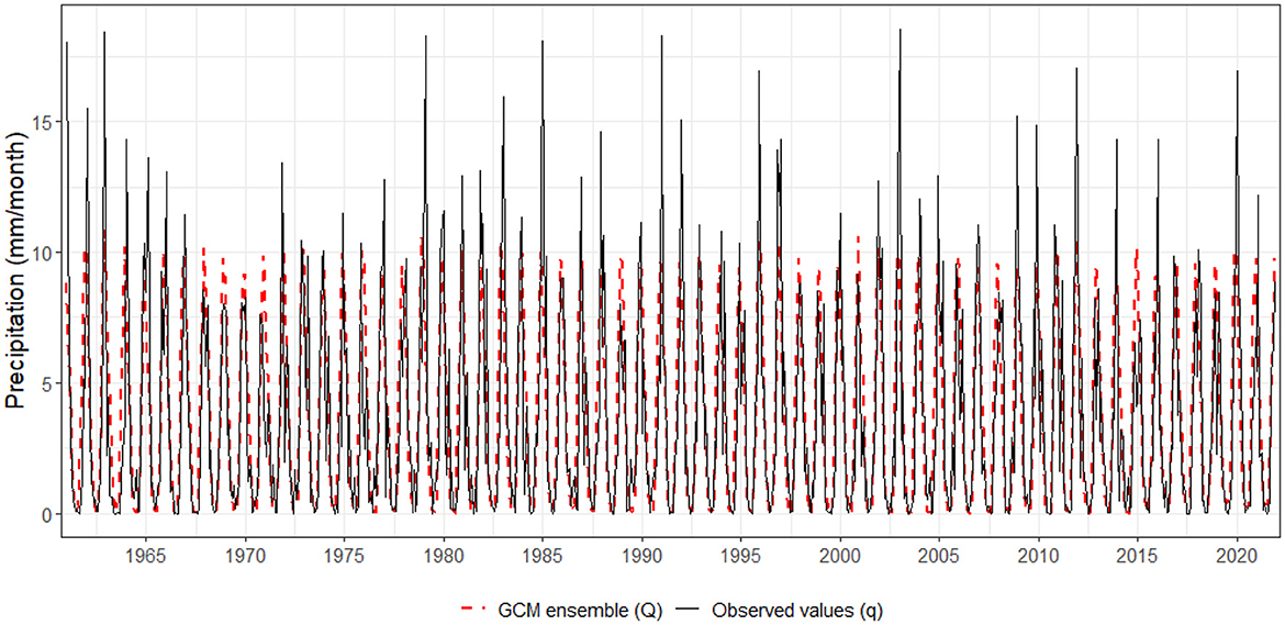
Figure 8. Realizations of variables q and Q for monthly rainfall.

Figure 9

Figure 9. Realizations of variables q and Q for monthly average temperature °C.

Next, we derived the empirical conditional distributions in Equation 5 for the period 1961–2011, after removing seasonal effects and transforming the original variables (Equation 8)—the estimated values of α are 21.07mm and 10.96°C for rainfall and temperature, respectively. Results are summarized in Figures 10, 11. For monthly rainfall, e-Bluecat was able to reproduce the local averages throughout the entire period. In fact, the model median estimates are in close agreement with those of the observed time series and are slightly larger than those of the GCM ensemble. In addition, apart from the largest rainfall amounts, the conditional distributions properly described the variability of the process—the empirical coverage probability is 86.8%, which is close to the theoretical one (90%). This suggests that e-Bluecat properly corrected the bias in the first moment of the ensemble and provided reasonable estimates of the conditional variances of rainfall amounts in the MRBH. However, the model is unable to simulate very wet conditions, which are important for replenishing soil moisture in agricultural areas within the MRBH and for providing water to the water supply systems reservoirs. Finally, the average width of the confidence intervals during the calibration stage amounts 6.47mm/day (after the backwards transformation with the inverse of Equation 8). Although this quantity is deemed too large, since we are dealing with a smoothed process (monthly time scale) which filters out the effects of extreme events, it will provide a baseline for assessing model performance in validation and extrapolation.

Figure 10

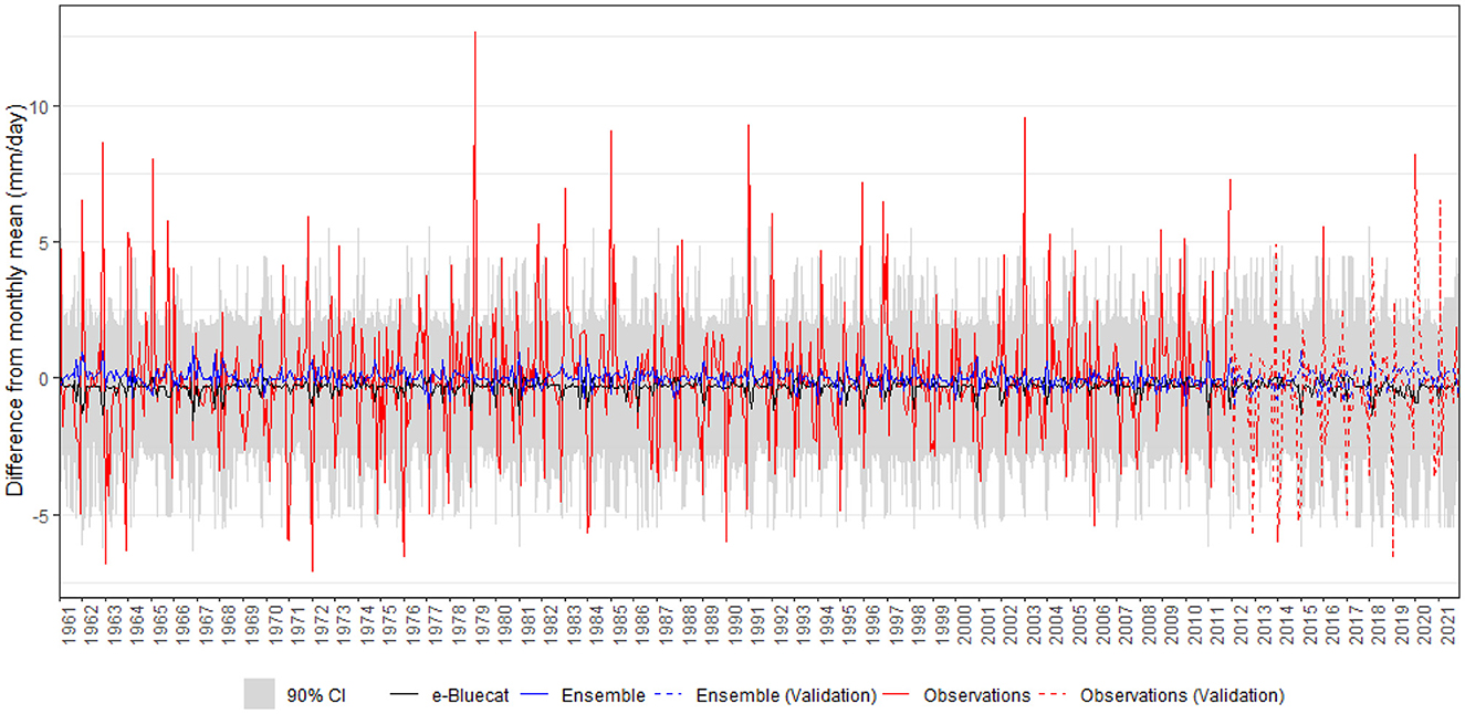
Figure 10. Comparation between GCM's ensemble and e-Bluecat realizations for rainfall.

Figure 11

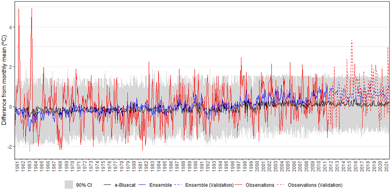
Figure 11. Comparation between GCM's ensemble and e-Bluecat realizations for temperature.

For monthly temperatures, the ensemble more strongly disagrees with the observed process, but, to some extent, e-Bluecat is able to approximate the local averages and reproduce the observed “trend,” particularly for the period after the year 2000, in which a more pronounced increasing trend is verified for the GCM estimates. The empirical coverage probability is 87.8%, which is slightly higher than that obtained for rainfall, but the model again could not reproduce the larger observed temperatures. The average width of the confidence intervals interval is 2.81°C (after the backwards transformation with the inverse of Equation 8), but the upper limits of the confidence intervals become more similar as the model more strongly departs from observations. This may be a direct result of the hot model problem (Hausfather et al., 2022)—the higher observed order statistics are similar for a wide range of increasing values of Q, which leads to similar conditional distributions (or at least the upper tails) during extrapolation. We also note that the lower limits of the confidence intervals move upwards for most of the period between 2000 and 2011 as a result of the extrapolation procedure, but there is much more variability in the 5th percentiles than in the 95th counterparts. A similar behavior was observed by Koutsoyiannis and Montanari (2022b) when applying e-Bluecat over the Italian territory.

We then proceeded to model validation in the period 2012–2021—note that the levels of extrapolation for the lower and higher order statistics (i.e., Q<Q_(m+1:N) and Q>Q_(N−m:N)) are similar to those in the calibration stage, which, to a great extent, preserves the parameter estimates obtained during model training. We again refer to Figures 10, 11 for discussing the results for rainfall and temperature, respectively. The empirical coverage probability for the former variable is 85.8%, which is slightly lower than in calibration, but the model is again able to reproduce the local averages. Also, the average width of the confidence intervals is only slightly wider in testing conditions, amounting 6.93mm/day (after the backwards transformation with the inverse of Equation 8). Overall, e-Bluecat appears to reliably extrapolate rainfall amounts in future scenarios in the MRBH, albeit the model could not properly reproduce the rainfall amounts in a few of the drier months after 2012—which was a very dry period in the Brazilian southeastern region.

For temperatures, e-Bluecat could not properly describe the local averages, more likely due to “opposite” behaviors between observations and GCM estimates during the testing stage. In effect, for many cases, high observed temperatures are associated with concurrent low estimates from the ensemble. This fact clearly indicates the limited ability of the climate projections in describing the actual evolution of the climate system in the RMBH and highlights the potential problems of utilizing deterministic bias-corrected estimates for decision-making, even under complex bias-correction techniques [see the discussion in Maraun et al. (2017)]—critical scenarios may not be disclosed because of the limited predictive abilities of the ensemble. On the other hand, the empirical coverage probability obtained with e-Bluecat, 85.8%, is still acceptable, which suggests that the process variability is reasonably accounted for by the model. In other words, although the bias in the first moment could not be entirely removed, the stochastic description offered by e-Bluecat circumvents the poor representation of the observed process through GCM point estimates and allows simulating more extreme events and observed “trends” almost irrespective of the behavior of the conditioning variable. At last, the average width of the confidence intervals during prediction, 2.71°C (after the backwards transformation with the inverse of Equation 8), is narrower than that obtained in model training. This may be again ascribed to the extrapolation procedure, which, as compared to the calibration stage, entailed relatively larger values for the 5th percentiles but very similar estimates for the 95th ones.

Finally, we calibrated the parameters of e-Bluecat considering the projection period (here assumed as 2022–2100), under the three climate change scenarios. Results are summarized in Table 1. One may notice that, for rainfall, the slopes a_l are positive and relatively close to 1 for all climate change scenarios, which indicates reasonable agreements among observations and ensemble estimates in the lower portions of the scatterplots. Parameters a_u are also positive for this variable, but the slopes approach zero for SSP2-4.5 and SSP5-8.5, which highlights the mismatches between the time series as Q increases. As a result, the conditional distributions become flatter for the larger rainfall amounts due to the limited explanatory ability of the climate model. We also note that the lower bound Q_l is considerably higher for SSP2-4.5, which suggests that, under this scenario, smaller deviations with respect to the mean values (i.e., less severe drought episodes, in terms of intensity) are expected during the projection period. On the other hand, the values of Q_u were similar for all scenarios, with a slightly larger estimate for the optimistic climate change scenario. This fact suggests that, at least at the monthly scale, the differences among emission scenarios are more strongly perceived during droughts in the MRBH.

Table 1

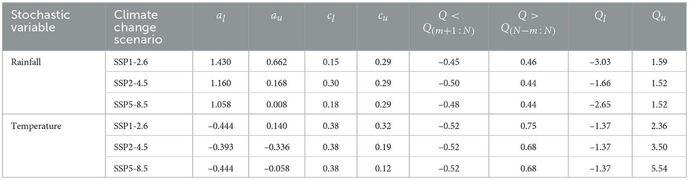
Table 1. Parameters of the e-Bluecat model and the corresponding ranges for extrapolation in the period 1961–2100.

For temperatures, slopes a_l and a_u are either negative (SSP2-4.5 and SSP5-8.5) or very close to zero (SSP1-2.6), which indicates that the ensemble cannot provide useful information for deriving the empirical conditional distributions in the extrapolation ranges—model estimates and observations follow opposite “trends.” We also note that, while the values of Q_l are similar for all climate change scenarios, the value of Q_u for SSP5-8.5 is more than twice that for SSP1-2.6 and roughly 1.5 times larger than that for SSP2-4.5. Hence, differences on GGC would imply a much stronger effect on temperatures than on rainfall amounts in the MRBH—depending on the trajectory of the process, as materialized by distinct climate change scenarios, the vulnerability of the water supply system to meteorological droughts may be greatly enhanced by the increased evaporation in the reservoirs. On the other hand, the extent to which these very distinct temporal dynamics are affected by the “hot model” problem (Hausfather et al., 2022) is not clear. As a result, some of these trajectories might be physically implausible, in view of the current empirical knowledge on climate dynamics—this further complicates developing strategies for drought mitigation in the study area.

Finally, Figure 12 illustrates the bias-corrected rainfall estimates during the projection period for the three climate change scenarios. Overall, the processes dynamics do not differ much from those of the historical time span—irrespective of the future GGC, no trends or variance changes are perceived, which suggests that the asymptotic behavior of the conditional distributions was fully captured during model calibration. However, the variability informed by the stochastic model is much larger than that predicted by the GCM ensemble, which could make the actual alternation between very dry and very wet years much more pronounced than anticipated by the climate models, further complicating future drought mitigation. As compared to the previous e-Bluecat runs, the average width of the confidence intervals is slightly larger for SSP1-2.6 (7.81mm/day) and SSP2-4.5 (7.22mm/day), but virtually the same for SSP5-8.5 (6.94mm/day)—these large ranges again translate the high levels of uncertainty associated with the climate models and highlight the difficulties for informing adaptation strategies, even after bias correction (Maraun et al., 2017). To sum up, based on results obtained with e-Bluecat, no marked changes in monthly rainfall patterns are expected in the MRBH. Nonetheless, it is possible to note physically implausible values for rainfall amounts in all scenarios, which indicates that the model misrepresents the probability dry and, as a result, the simulation of long dry spells may be hindered. This is surely a limitation of the proposed approach in regions with strong seasonal characteristics, such as the MRBH. However, adapting model structures for encompassing mixed discrete-continuous distributions would require alternative approaches for addressing seasonality (cyclostationarity) and autocorrelation, which could severely reduce the number of sample points for deriving the conditional distributions.

Figure 12

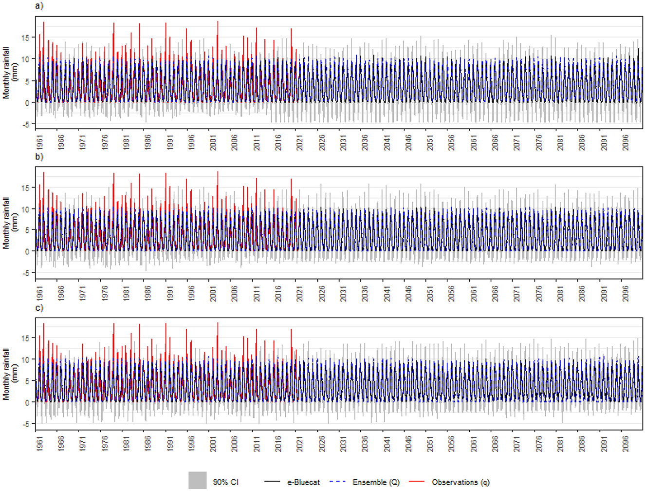
Figure 12. Bluecat results—monthly mean of rainfall (A) for scenario SSP1-2.6. (B) For scenario SSP2-4.5. (C) For scenario SSP5-8.5.

For monthly temperatures (Figure 13), on the other hand, increasing “trends” are verified in the bias-corrected projections, at least for some periods in the future, for all climate change scenarios. For SSP1-2.6, median temperatures are expected to increase up to the 2050s and then stabilize. It is worth noting, however, that, while the ensemble predicts an average increase of ~2°C, e-Bluecat estimates suggest this quantity would not surpass 0.5°C at the end of the projection period. For SSP2-4.5, the median temperature estimates steadily increase throughout the projection period, albeit at a much lower rate than that predicted by the ensemble—the former amounts an increase of < 1°C in 2100 whereas the latter indicates almost 4°C. Finally, for SSP5-8.5, which also increases during the entire projection period, but much more steeply than in the baseline scenario, the climate model suggests an average increase of more than 5°C in 2100; e-Bluecat, in turn, again points to < 1°C. On the other hand, the variability inferred by e-Bluecat is again much larger than that predicted by the climate models, which may complicate the mechanisms of water transport to the atmosphere and the water budget in the water supply system reservoirs. Finally, for all scenarios, the average width of the confidence intervals is 2.8°C, which suggests that the asymptotic behavior of the conditional distributions is also captured for temperatures during calibration, despite the larger disagreement among observations and climate model estimates for this variable in the historical period.

Figure 13

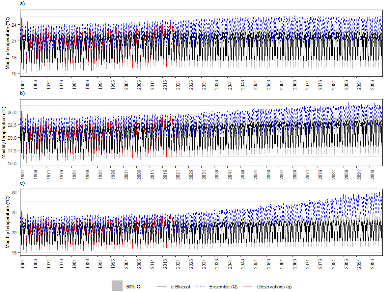
Figure 13. Bluecat results—monthly mean of temperature (A) for scenario SSP1-2.6. (B) For scenario SSP2-4.5. (C) For scenario SSP5-8.5.

Based on our results, the main difficulty for future drought mitigation and adaptation in the MRBH would not be related to changes in the processes' averages, which are expected to vary smoothly over time, but rather to the much higher variability predicted by the stochastic model as compared to GCM projections. Increased variability, along with the processes' persistence, might lead to longer periods with very low rainfall amounts and very high temperatures, worsening drought conditions and impacting the region's economy and environment. This fact highlights the importance of simulation, which is possible with the e-Bluecat framework, for tracking critical yet physically plausible trajectories for the processes and for defining more effective adaptation strategies in the study area. Moreover, the high uncertainty levels in future projections, as translated by the large variances of the conditional distributions for both stochastic variables, suggests that deterministic bias-correction only may hinder risk assessment and communication and misinform decision-making.

4 Discussion

Climate projections predict diminishing precipitation and rising temperatures in the following decades in several areas across the world, (IPCC, 2023), with potential increases in the frequencies of drought events, as well as in their durations and severities. Prolonged drought conditions, in turn, may strongly affect rainfall-runoff relationships (e.g., Deb et al., 2019), which would impose additional challenges for water resources management under changing climate and more intricate drought dynamics. This situation is critical in urban and periurban areas, such as the MRBH, due to their high demands for water (Nobre et al., 2016) and their usual dependence on reservoirs for multiple water uses. On the other hand, climate projections, as obtained from GCMs, are acknowledged biased and uncertain (Koutsoyiannis and Montanari, 2022b), particularly for small areas with marked seasonality in hydroclimatic processes. As a result, effective bias-correction techniques, preferably with formal mechanisms for uncertainty estimation, become necessary for devising strategies for future drought mitigation and adaptation in such areas.

This study was built upon the drawbacks of using deterministic GCM-based forecasts to establish management plans for water resources in the MRBH. Possible effects of wrongful projections of rainfall and temperature may lead to important implications for watersheds. Among them, one may cite the inaccurate predictions of surface water supply (Liu et al., 2021), unreliable assessment of impacts on ecosystems' stability and water availability due to the rainfall-related reorganization of river network reorganization (Abed-Elmdoust et al., 2016), and poor representation of nutrient load dynamics in water supply reservoirs (Miralha et al., 2021). To some extent, the stochastic representation provided by e-Bluecat in our application circumvents these problems, as it allows simulating distinct trajectories of the processes of interest and testing alternatives on a probability-consequence basis.

Our results suggested that, on average terms and irrespective of the considered climate change scenario, no significant changes would be observed in monthly rainfall amounts and only small increases (~1°C) would be verified in monthly temperatures. To a great extent, these results contrast with deterministic approaches for bias-correction, which mostly indicate more pronounced increases in temperatures and more noticeable variations in rainfall in other parts of the world (e.g., Deb et al., 2018; Dai et al., 2022), as well as a stronger influence of the radiative forcing levels on the future trajectories of the processes (e.g., Bukovsky et al., 2021; Dinh and Aires, 2023). On the other hand, the stochastic bias-correction approach utilized in this study suggested a much larger variability for both future temperature and rainfall, which might reflect the long-range persistence associated with these processes (Koutsoyiannis, 2023) and may enhance the likelihood of severe and extreme drought events in the future. This fact highlights the limited predictive abilities of deterministically bias-corrected climate projections (Maraun et al., 2017) and their potentially small effectiveness for decision-making (Koutsoyiannis and Montanari, 2022b). Also, properly accounting for uncertainty in climate projections comprises a key step for modeling possible changes in the mechanisms of water transferring through atmosphere, soils, streams and aquifers during severe multiyear droughts (Deb et al., 2019, 2022).

On the other hand, the marked seasonal characteristics of climate in the MRBH entailed physically inconsistent estimates when bias-correcting rainfall amounts, even for a relatively coarse temporal resolution (monthly) for rainfall aggregation. Such a limitation has not been reported in previous research with e-Bluecat (Koutsoyiannis and Montanari, 2022b) and suggests that, under some circumstances, devising cyclostationary models might be unavoidable. It should also be noted that e-Bluecat was unable to reproduce very large rainfall amounts and temperatures—which is an obvious result of its essentially empirical nature. However, deterministic bias correction techniques often cannot also map high GCM quantiles in a physically meaningful way (Maraun, 2016), and this remains an unresolved issue in the literature (e.g., Dinh and Aires, 2023). Based on these arguments, utilizing e-Bluecat in other areas, with distinct climate characteristics, is feasible, albeit the model appears to perform better when seasonality is less pronounced [see the discussion in Koutsoyiannis and Montanari (2022b)].

Finally, from a practical perspective, our results might be useful to strengthen the MRBH's water supply system by implementing early drought warning systems using e-Bluecat's probabilistic analyses, and developing robust contingency plans that account for climate projection uncertainties (Di Baldassarre et al., 2018). At the same time, adaptive water management in the MRBH must consider both anthropogenic climate change and land use changes [current limitations on this are discussed in Deb et al. (2018)]. For instance, Magaña et al. (2021) pointed out that expanding metropolitan areas need integrated approaches combining technical and socioeconomic aspects of drought management. Furthermore, to enhance the adaptive management of the study area in response to climate change, selecting appropriate locations for hydrologic monitoring is paramount (Singhal et al., 2024). At last, to maintain the long-term environmental integrity of river basins, Gao et al. (2022) also stress the necessity of assessing dam development and water infrastructure design in light of unknown climate dynamics.

5 Conclusions

The findings of this study highlight both the limitations and potential of the e-Bluecat model for bias correction and uncertainty quantification in climate projections in small areas with marked seasonality. The stochastic representation of precipitation and temperature in the MRBH revealed the following key points:

• Global climate models (GCM) demonstrated notable limitations in reproducing observed processes. For precipitation, there was a systematic underestimation of maximum monthly amounts and an inadequate representation of its variability. Regarding temperature, the “hot model” problem emerged, with future projections showing physically disputable upward trends. Also, the variance was again misrepresented for this variable;

• The e-Bluecat model effectively corrected bias of the first moment (mean) for precipitation, and provided empirical coverage close to theoretical levels (86.8%–87.8%). However, the confidence intervals for both precipitation and temperature revealed large uncertainty, especially under extrapolation conditions. Additionally, e-Bluecat struggled to fully reproduce observed extreme values, reflecting the inherent limitations from GCMs;

• Across the three climate change scenarios (SSP1-2.6, SSP2-4.5, and SSP5-8.5), e-Bluecat captured, to a great extent, the asymptotic behavior of the conditional distributions for precipitation in the study area. No significant shifts in monthly precipitation patterns were observed, even under the most extreme scenarios. In contrast, temperature projections indicated progressive increases, albeit at much smaller rates than those predicted by GCMs. This highlights e-Bluecat's potential to temper exaggerated predictions in the most pessimistic scenarios;

• e-Bluecat's stochastic structure proved an useful tool for capturing climate variability and simulating extreme events, despite the frequent disagreement among GCM outputs and observations. In fact, these discrepancies indicate the need for caution when applying deterministic bias-corrected estimates in strategic decisions, particularly in sensitive contexts such as water resource management and drought mitigation in the MRBH;

• Despite e-Bluecat's relative success, uncertainties remain regarding the physical plausibility of certain projected trajectories, particularly for temperature. The challenges of extrapolation and inconsistencies between climate scenarios call for continuous efforts to improve climate model representativeness and develop more advanced bias correction techniques.

On the other hand, the stochastic representation provided by e-Bluecat has still some limitations. First, the essentially empirical approach for estimating the conditional distributions hinders extrapolation to very extreme levels of the modeled processes. In the context of future drought assessment in the MRBH, this might conceal the effects of very high temperatures in evaporation and, accordingly, in water availability in the water supply reservoirs. Moreover, the simplified approach for dealing with seasonality implied physically implausible values for monthly precipitation amounts. This would call for a more structured model for dealing with the probability dry during the dry seasons in the study area. However, inference would be affected by loss of information as the cyclostationarity of the processes is formally accounted for. Finally, the use of a simple averaging over models for building the GCM ensemble might have led to oversmoothed trajectories for the climate projections. The use of alternative approaches for selecting more influential members among the available climate models (e.g., Sa'adi et al., 2024) could improve the representativeness of the ensemble with respect to the observed processes.

The application of e-Bluecat for bias correction of temperature and precipitation in a small area with a complex climate, such as the RMBH, demonstrated its predictive skills and generalization abilities, and highlighted some limitations. More importantly, however, is that our results indicate that climate-related planning strategies must necessarily account for the high levels of uncertainty related to GCM outputs for defining critical trajectories of hydroclimatic processes and, accordingly, optimizing the allocation of financial resources for drought adaptation and mitigation.

Data availability statement

The raw data supporting the conclusions of this article will be made available by the authors, without undue reservation.

Author contributions

LS: Conceptualization, Formal analysis, Investigation, Methodology, Software, Writing – original draft, Writing – review & editing. AB: Formal analysis, Investigation, Visualization, Writing – original draft, Writing – review & editing. CL: Investigation, Visualization, Writing – original draft. GS: Investigation, Visualization, Writing – original draft. EM: Funding acquisition, Investigation, Visualization, Writing – original draft. VC: Conceptualization, Formal analysis, Funding acquisition, Investigation, Methodology, Resources, Supervision, Visualization, Writing – original draft, Writing – review & editing.

Funding

The author(s) declare that financial support was received for the research and/or publication of this article. This paper was funded by CNPq (grant number: 440013/2024-0) and FAPESP (grant number: 2022/08468-0).

Acknowledgments

We express our gratitude to Professor Demetris Koutsoyiannis for the helpful interaction during the early stages of our research. We also acknowledge the support to this research from Conselho Nacional de Desenvolvimento Científico e Tecnológico (CNPq), Coordenação de Aperfeiçoamento de Pessoal de Nível Superior (CAPES), Fundação de Amparo à Pesquisa do Estado de Minas Gerais (FAPEMIG), and Fundação de Amparo à Pesquisa do Estado de São Paulo (FAPESP). We also wish to acknowledge the reviewers and editors for the valuable comments and suggestions, which greatly helped improve the paper.

Conflict of interest

The authors declare that the research was conducted in the absence of any commercial or financial relationships that could be construed as a potential conflict of interest.

Generative AI statement

The author(s) declare that no Gen AI was used in the creation of this manuscript.

Publisher's note

All claims expressed in this article are solely those of the authors and do not necessarily represent those of their affiliated organizations, or those of the publisher, the editors and the reviewers. Any product that may be evaluated in this article, or claim that may be made by its manufacturer, is not guaranteed or endorsed by the publisher.

References

Abed-Elmdoust, A., Miri, M., and Singh, A. (2016). Reorganization of river networks under changing spatiotemporal precipitation patterns: an optimal channel network approach. Water Resour. Res. 52, 8845–8860. doi: 10.1002/2015WR018391

Crossref Full Text | Google Scholar

ANA (2024). Hidroweb - sistema de informações hidrológicas (Brasília).

Google Scholar

Bastola, S., Murphy, C., and Sweeney, J. (2011). The role of hydrological modelling uncertainties in climate change impact assessments of Irish river catchments. Adv. Water Resour. 34, 562–576. doi: 10.1016/j.advwatres.2011.01.008

Crossref Full Text | Google Scholar

Brêda, J. P. L. F., De Paiva, R. C. D., Collischon, W., Bravo, J. M., Siqueira, V. A., and Steinke, E. B. (2020). Climate change impacts on south American water balance from a continental-scale hydrological model driven by CMIP5 projections. Clim. Change 159, 503–522. doi: 10.1007/s10584-020-02667-9

Crossref Full Text | Google Scholar

Bukovsky, M. S., Gao, J., Mearns, L. O., and O'Neill, B. C. (2021). SSP–based land-use change scenarios: a critical uncertainty in future regional climate change projections. Earths Future 9:e2020EF001782. doi: 10.1029/2020EF001782

Crossref Full Text | Google Scholar

Chiew, F. H. S., Zheng, H., Potter, N. J., Charles, S. P., Thatcher, M., Ji, F., et al. (2022). Different hydroclimate modelling approaches can lead to a large range of streamflow projections under climate change: Implications for water resources management. Water 14:2730. doi: 10.3390/w14172730

Crossref Full Text | Google Scholar

Dai, C., Qin, X., Zhang, X., and Liu, B. (2022). Study of climate change impact on hydro-climatic extremes in the Hanjiang river basin, China, using Cordex-EAS data. Weather Clim. Extrem. 38:100509. doi: 10.1016/j.wace.2022.100509

Crossref Full Text | Google Scholar

Deb, P., Babel, M. S., and Denis, A. F. (2018). Multi-GCMS approach for assessing climate change impact on water resources in Thailand. Model. Earth Syst. Environ. 4, 825–839. doi: 10.1007/s40808-018-0428-y

Crossref Full Text | Google Scholar

Deb, P., Kiem, A. S., and Willgoose, G. (2019). Mechanisms influencing non-stationarity in rainfall-runoff relationships in southeast Australia. J. Hydrol. 571, 749–764. doi: 10.1016/j.jhydrol.2019.02.025

Crossref Full Text | Google Scholar

Deb, P., Moradkhani, H., Han, X., Abbaszadeh, P., and Xu, L. (2022). Assessing irrigation mitigating drought impacts on crop yields with an integrated modeling framework. J. Hydrol. 609, 127760. doi: 10.1016/j.jhydrol.2022.127760

Crossref Full Text | Google Scholar

Di Baldassarre, G., Wanders, N., AghaKouchak, A., Kuil, L., Rangecroft, S., Veldkamp, T. I. E., et al. (2018). Water shortages worsened by reservoir effects. Nat. Sustain. 1, 617–622. doi: 10.1038/s41893-018-0159-0

PubMed Abstract | Crossref Full Text | Google Scholar

Dinh, T. L. A., and Aires, F. (2023). Revisiting the bias correction of climate models for impact studies. Clim. Change 176:140. doi: 10.1007/s10584-023-03597-y

Crossref Full Text | Google Scholar

Gabric, A. J. (2023). The climate change crisis: a review of its causes and possible responses. Atmosphere 14:1081. doi: 10.3390/atmos14071081

Crossref Full Text | Google Scholar

Gao, Y., Sarker, S., Sarker, T., and Leta, O. T. (2022). Analyzing the critical locations in response of constructed and planned dams on the Mekong river basin for environmental integrity. Environ. Res. Commun. 4:101001. doi: 10.1088/2515-7620/ac9459

Crossref Full Text | Google Scholar

Gesualdo, G. C., Benso, M. R., Sass, K. S., and Mendiondo, E. M. (2024). Index-based insurance to mitigate current and future extreme events financial losses for water utilities. Int. J. Disaster Risk Reduct. 100:104218. doi: 10.1016/j.ijdrr.2023.104218

Crossref Full Text | Google Scholar

Hausfather, Z., Marvel, K., Schmidt, G. A., Nielsen-Gammon, J. W., and Zelinka, M. (2022). Climate simulations: recognize the ‘hot model' problem. Nature 605, 26–29. doi: 10.1038/d41586-022-01192-2

PubMed Abstract | Crossref Full Text | Google Scholar

Hersbach, H., Bell, B., Berrisford, P., Hirahara, S., Horányi, A., Muñoz-Sabater, J., et al. (2020). The era5 global reanalysis. Q. J. R. Meteorol. Soc. 146, 1999–2049. doi: 10.1002/qj.3803

Crossref Full Text | Google Scholar

INMET (2024). Banco de dados meteorológicos (Brasília).

Google Scholar

IPCC (2023). Climate Change 2023: Synthesis Report. Geneva: Intergovernmental Panel on Climate Change.

Google Scholar

Koutsoyiannis, D. (2010). Hess opinions “a random walk on water”. Hydrol. Earth Syst. Sci. 14, 585–601. doi: 10.5194/hess-14-585-2010

Crossref Full Text | Google Scholar

Koutsoyiannis, D. (2023). Stochastics of Hydroclimatic Extremes - A Cool Look at Risk, 3rd Edn. Athens: Kallipos, Open Academic Editions.

Google Scholar

Koutsoyiannis, D., and Montanari, A. (2022a). Bluecat: a local uncertainty estimator for deterministic simulations and predictions. Water Resour. Res. 58:e2021WR031215. doi: 10.1029/2021WR031215

Crossref Full Text | Google Scholar

Koutsoyiannis, D., and Montanari, A. (2022b). Climate extrapolations in hydrology: the expanded bluecat methodology. Hydrology 9:86. doi: 10.3390/hydrology9050086

Crossref Full Text | Google Scholar

Kusch, E., and Davy, R. (2022). Krigr—a tool for downloading and statistically downscaling climate reanalysis data. Environ. Res. Lett. 17:024005. doi: 10.1088/1748-9326/ac48b3

Crossref Full Text | Google Scholar

Liu, Z., Herman, J. D., Huang, G., Kadir, T., and Dahlke, H. E. (2021). Identifying climate change impacts on surface water supply in the Southern Central Valley, California. Sci. Total Environ. 759:143429. doi: 10.1016/j.scitotenv.2020.143429

PubMed Abstract | Crossref Full Text | Google Scholar

Magaña, V., Herrera, E., Ábrego Góngora, C. J., and Ávalos, J. A. (2021). Socioeconomic drought in a mexican semi-arid city: monterrey metropolitan area, a case study. Front. Water 3:579564. doi: 10.3389/frwa.2021.579564

Crossref Full Text | Google Scholar

Malede, D. A., Andualem, T. G., Yibeltal, M., Alamirew, T., Kassie, A. E., Demeke, G. G., et al. (2024). Climate change impacts on hydroclimatic variables over a wash basin, Ethiopia: a systematic review. Disc. Appl. Sci. 6. doi: 10.1007/s42452-024-05640-8

Crossref Full Text | Google Scholar

Maraun, D. (2016). Bias correcting climate change simulations - a critical review. Curr. Clim. Change Rep. 2, 211–220. doi: 10.1007/s40641-016-0050-x

PubMed Abstract | Crossref Full Text | Google Scholar

Maraun, D., Shepherd, T. G., Widmann, M., Zappa, G., Walton, D., Gutiérrez, J. M., et al. (2017). Towards process-informed bias correction of climate change simulations. Nat. Clim. Change 7, 764–773. doi: 10.1038/nclimate3418

Crossref Full Text | Google Scholar

Maurer, E. P., and Pierce, D. W. (2014). Bias correction can modify climate model simulated precipitation changes without adverse effect on the ensemble mean. Hydrol. Earth Syst. Sci. 18, 915–925. doi: 10.5194/hess-18-915-2014

Crossref Full Text | Google Scholar

Miralha, L., Muenich, R. L., Scavia, D., Wells, K., Steiner, A. L., Kalcic, M., et al. (2021). Bias correction of climate model outputs influences watershed model nutrient load predictions. Sci. Total Environ. 759:143039. doi: 10.1016/j.scitotenv.2020.143039

PubMed Abstract | Crossref Full Text | Google Scholar

Montanari, A., and Koutsoyiannis, D. (2014). Modeling and mitigating natural hazards: stationarity is immortal! Water Resour. Res. 50, 9748–9756. doi: 10.1002/2014WR016092

Crossref Full Text | Google Scholar

Muerth, M. J., Gauvin St-Denis, B., Ricard, S., Velázquez, J. A., Schmid, J., Minville, M., et al. (2013). On the need for bias correction in regional climate scenarios to assess climate change impacts on river runoff. Hydrol. Earth Syst. Sci. 17, 1189–1204. doi: 10.5194/hess-17-1189-2013

Crossref Full Text | Google Scholar

Naghettini, M. (Ed.). (2017). Fundamentals of Statistical Hydrology. Cham: Springer International Publishing. doi: 10.1007/978-3-319-43561-9

Crossref Full Text | Google Scholar

Nobre, C. A., Marengo, J. A., Seluchi, M. E., Cuartas, L. A., and Alves, L. M. (2016). Some characteristics and impacts of the drought and water crisis in southeastern brazil during 2014 and 2015. J. Water Resour. Protect. 08, 252–262. doi: 10.4236/jwarp.2016.82022

Crossref Full Text | Google Scholar

Rajulapati, C. R., and Papalexiou, S. M. (2023). Precipitation bias correction: a novel semi-parametric quantile mapping method. Earth Space Sci. 10:e2023EA002823. doi: 10.1029/2023EA002823

Crossref Full Text | Google Scholar

Rama Nemani, N. (2021). NASA earth exchange global daily downscaled projections - CMIP6. doi: 10.7917/OFSG3345

Crossref Full Text | Google Scholar

Rodrigues, R. R., Taschetto, A. S., Sen Gupta, A., and Foltz, G. R. (2019). Common cause for severe droughts in south America and marine heatwaves in the south Atlantic. Nat. Geosci. 12, 620–626. doi: 10.1038/s41561-019-0393-8

Crossref Full Text | Google Scholar

Sa'adi, Z., Alias, N. E., Yusop, Z., Iqbal, Z., Houmsi, M. R., Houmsi, L. N., et al. (2024). Application of relative importance metrics for CMIP6 models selection in projecting basin-scale rainfall over johor river basin, malaysia. Sci Total Environ. 912:169187. doi: 10.1016/j.scitotenv.2023.169187

PubMed Abstract | Crossref Full Text | Google Scholar

Sarker, S. (2022). Fundamentals of climatology for engineers: lecture note. Eng, 3, 573–595. doi: 10.3390/eng3040040

Crossref Full Text | Google Scholar

Singhal, A., Jaseem, M., Divya Sarker, S., Prajapati, P., Singh, A., and Jha, S. K. (2024). Identifying potential locations of hydrologic monitoring stations based on topographical and hydrological information. Water Resour. Manag. 38, 369–384. doi: 10.1007/s11269-023-03675-x

Crossref Full Text | Google Scholar

Tegegne, G., Kim, Y., and Lee, J. (2019). Spatiotemporal reliability ensemble averaging of multimodel simulations. Geophys. Res. Lett. 46, 12321–12330. doi: 10.1029/2019GL083053

PubMed Abstract | Crossref Full Text | Google Scholar

Tegegne, G., and Melesse, A. M. (2020). Multimodel ensemble projection of hydro-climatic extremes for climate change impact assessment on water resources. Water Resour. Manag. 34, 3019–3035. doi: 10.1007/s11269-020-02601-9

Crossref Full Text | Google Scholar

Thrasher, B., Wang, W., Michaelis, A., Melton, F., Lee, T., Nemani, R., et al. (2022). Nasa global daily downscaled projections, cmip6. Sci. Data 9:262. doi: 10.1038/s41597-022-01393-4

PubMed Abstract | Crossref Full Text | Google Scholar

Wang, H., Chen, J., Xu, C., Zhang, J., and Chen, H. (2020). A framework to quantify the uncertainty contribution of GCMs over multiple sources in hydrological impacts of climate change. Earth Future 8:e2020EF001602. doi: 10.1029/2020EF001602

Crossref Full Text | Google Scholar

Wood, A. W., Leung, L. R., Sridhar, V., and Lettenmaier, D. P. (2004). Hydrologic implications of dynamical and statistical approaches to downscaling climate model outputs. Clim. Change 62, 189–216. doi: 10.1023/B:CLIM.0000013685.99609.9e

Crossref Full Text | Google Scholar

Xu, L., and Wang, A. (2019). Application of the bias correction and spatial downscaling algorithm on the temperature extremes from CMIP5 multimodel ensembles in China. Earth Space Sci. 6, 2508–2524. doi: 10.1029/2019EA000995

Crossref Full Text | Google Scholar

Xu, Y. (2015). hyfo: Hydrology and Climate Forecasting. Comprehensive R Archive Network. doi: 10.32614/CRAN.package.hyfo

Crossref Full Text | Google Scholar