The optimal location of tanks in water distribution networks using failure tolerance

The location of tanks impacts the optimal design and reliability of water distribution networks. However, contention exists in the literature regarding the best location for tanks. The aim of this study was therefore to develop a tool to compute failure tolerance when pipe failure occurs in a water distribution network, and as a consequence, to determine the optimal location of a tank(s). To achieve this, five optimal designs of the Anytown Network (ATN), which is a benchmark water distribution network in the literature, were selected. These designs, which recommended additional tanks at different locations of the network, were hydraulically simulated using pressure driven analysis in EPANET 2.2, and these results validated. To compute failure tolerance, a Microsoft Excel^® tool was developed, validated and applied to the hydraulically simulated results of the optimal ATN designs. The comparison of the failure tolerance values generated revealed the influence of tank location on the ATN reliability during pipe failure i.e., while each optimal ATN design generated a failure tolerance > 0.68 (a less vulnerable network), the best location for an additional tank(s) was downstream of the demand center. Incidentally, this design emerged as the cheapest and therefore points to the fact that a higher network reliability need not be a more expensive network.

1 Introduction

The location of tanks is integral to the optimal design and reliability of water distribution networks (WDNs) (Abunada et al., 2014; Curtin, 2024) and can significantly impact capital and recurrent costs (Walski et al., 1987; Murphy et al., 1994; Marlim and Kang, 2023). A large number of studies addressing the optimal design of WDNs have however focused on pumps, valves, and the sizing of pipes and tanks (Siew et al., 2016). Some of these studies include Saldarriaga et al. (2019), who considered the optimal design of WDNs while focused on the location of valves; Singh and Kekatos (2019) who considered pump sizing and operation; Ilemobade and Stephenson (2006) and van Dijk et al. (2008) who considered the optimal design of pipes; and van Zyl et al. (2008) who considered tank sizing. The implication of the limited research and guidelines into the optimal location of tanks within WDNs means that designers tend to rely on engineering judgement and experience to select the best location for tanks (Ajitha and Viji, 2023; Torkomany et al., 2020; Walski et al., 1987).

Research on tank design and location was pioneered by several researchers including Walters et al. (1999); Farmani et al. (2005); Vamvakeridou-Lyroudia et al. (2007); Basile et al. (2008); Prasad (2010); van Zyl (2014), and Mabrok et al. (2022). The below guidelines ensued from these studies:

a. Tank dimensioning is often specified by standards, with each country specifying its own tank size requirements, which often depend on the amount of water required for equalization, fire protection and non-fire emergencies (van Zyl, 2014).

b. Tank locations can be selected manually. However, it should be on higher ground in order to provide adequate pressure to the network (van Zyl, 2014; Mabrok et al., 2022). This guideline, however, leaves room for the ill-placement of tanks, and according to Abunada et al. (2014), an ill-placed tank can increase the total cost of a WDN while decreasing reliability.

c. Similar to (b), some studies recommend locating tanks upstream of the demand center and at the WDN's highest elevation (Darweesh, 2021). This view is echoed in the studies by Spedaletti et al. (2021) and Mabrok et al. (2022) who argue that, in practice, the best location of tanks is usually obvious and is well-known to be the highest elevation point in the WDN.

d. Tanks can be located at the demand center, typically found at the central section of a community (Singh and Kekatos, 2019). This is because the demand center, which represents the major demand area, generally experiences the highest demand for water. However, Seyoum et al. (2014) noted that although this approach to selecting the tank location may be conservative, it may lead to an infeasible solution since the demand center may not always have the desired conditions that will ensure minimum pressures are met throughout the WDN. Similar studies in this respect (e.g., Murphy et al., 1994; Vamvakeridou-Lyroudia et al., 2007; Basile et al., 2008) have concurred with this view.

e. Tanks can be located upstream and/or downstream of the demand center (Walters et al., 1999; Farmani et al., 2005; Prasad, 2010; Siew et al., 2016). These researchers found that the key benefit of placing tanks at these locations is that it improves network reliability in the event of transmission mains pipe breakdown.

Using the Anytown Network (ATN) as an example, Figure 1 shows the recommended locations of tanks by Murphy et al. (1994) (M), Walters et al. (1999) (W), Farmani et al. (2005) (F), Vamvakeridou-Lyroudia et al. (2007) (V), Basile et al. (2008) (B), Prasad (2010) (P), Siew et al. (2016) Design 1 (S1), Siew et al. (2016) Design 2 (S2), and Darweesh (2021) (D).

Figure 1

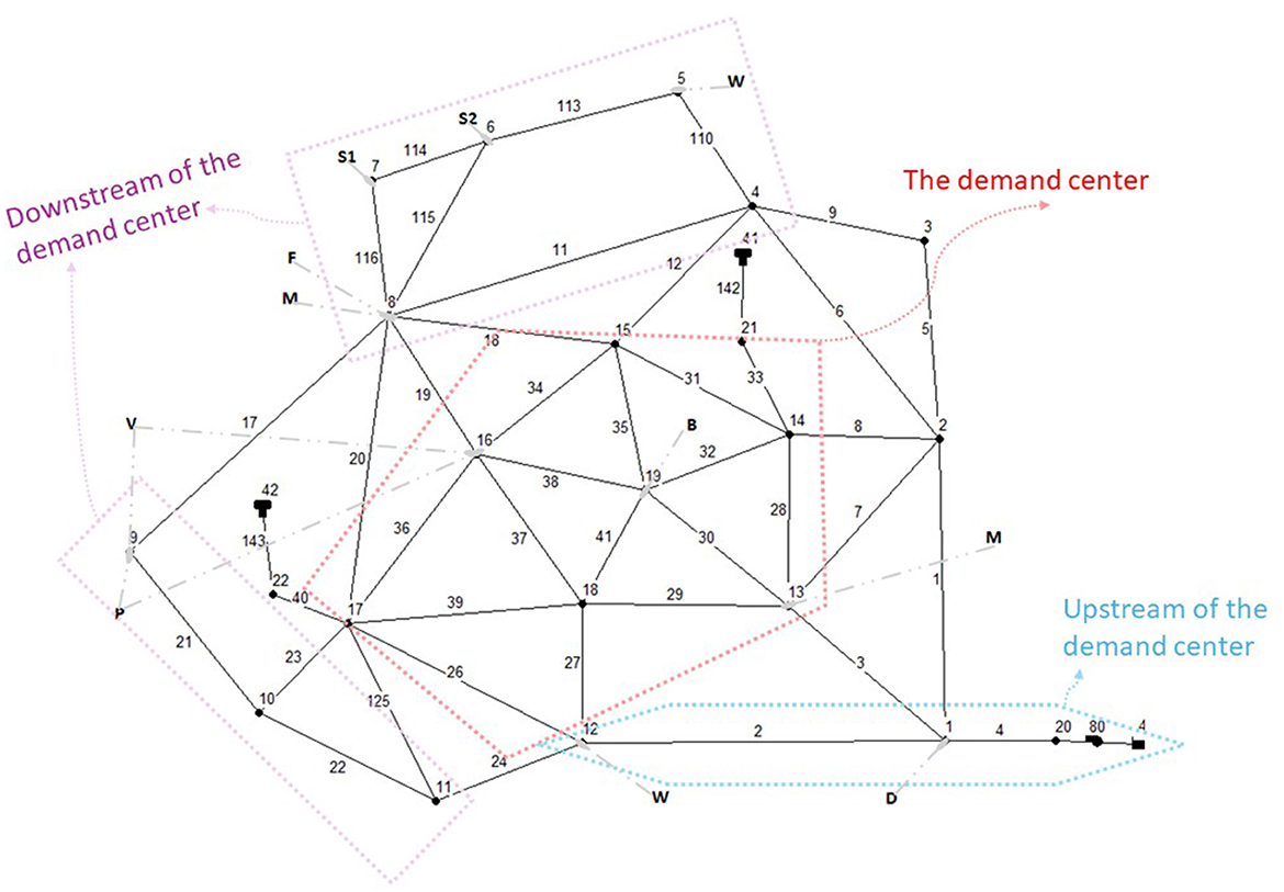
Figure 1. The ATN with tank locations from different studies (adapted from Walski et al., 1987).

The above guidelines show that the optimal location for tanks within WDNs is inconclusive. This study was therefore aimed at developing a tool to compute hydraulic reliability and failure tolerance of WDNs when a specific pipe fails, and as a consequence, to determine the optimal location of tanks within WDNs. The development and validation of this tool is explained in detail below.

2 Methodology

To address the aim of this study, the below methodology, consisting of four phases, was employed:

Phase (i) —the first phase of this study involved developing an algorithm. After development, the algorithm was employed to determine from literature, a benchmark WDN that has several optimal designs with tanks at different locations within the network.

Phase (ii) —The second phase involved employing EPANET 2.2 (Rossman, 2000) to hydraulically simulate the different optimal designs for the benchmark WDN obtained in phase (i) and comparing the simulated results with those published in the literature. Phase (ii) is important because hydraulic balancing of the selected benchmark WDN designs is a pre-requisite for computing hydraulic reliability and failure tolerance.

Phase (iii) —Using the reliability equations developed by Tanyimboh (1993) and Cullinane et al. (1992), phase (iii) involved developing a decision support tool (using Microsoft Excel^®) for computing the hydraulic reliability and failure tolerance of WDNs. This tool was validated by comparing the values it generated for certain Simple Network, SN (Figure 2) designs with the values generated by Tanyimboh and Setiadi (2008) for the same SN designs.

Phase (iv) —After conclusion of phases (i), (ii) and (iii), phase (iv) involved applying the developed Microsoft Excel^® tool to compute the hydraulic reliability and failure tolerance of the different optimal designs for the generic WDN obtained in phase (i). The results obtained in this phase, addressed the aim of this study i.e., to determine the optimal location of tanks in WDNs.

Figure 2

Figure 2. The Simple Network with nodal demands (l/s) (Tanyimboh and Templeman, 2000).

2.1 Phase (i)

As mentioned, phase (i) involved the development of an algorithm that determined from literature, a benchmark WDN that has several optimal designs with tanks at different locations within the network.

The ATN (Figure 1) is a hypothetical WDN situated in the Anytown community, USA and was selected as the benchmark WDN to be employed in phases (i), (ii), and (iv). Its details were retrieved from Walski et al. (1987).

Several ATN designs exist in the literature (Siew et al., 2016). The algorithm shown in Figure 3 was developed and employed to determine ATN designs that were hydraulically balanced and optimal, with tanks at different locations within the network. “Hydraulically balanced” refers to designs that satisfied the conservation of mass and energy, and met the minimum pressure threshold for the loading conditions outlined in the Battle of the Network Models: Epilog (Walski et al., 1987). “Optimal” refers to designs that cost ≤ $11 million. The ceiling of $11 million was selected because, while the least cost optimal ATN design published in Walski et al. (1987) was > $11 million, other optimal designs that cost < $11 m have since emerged in the literature.

Figure 3

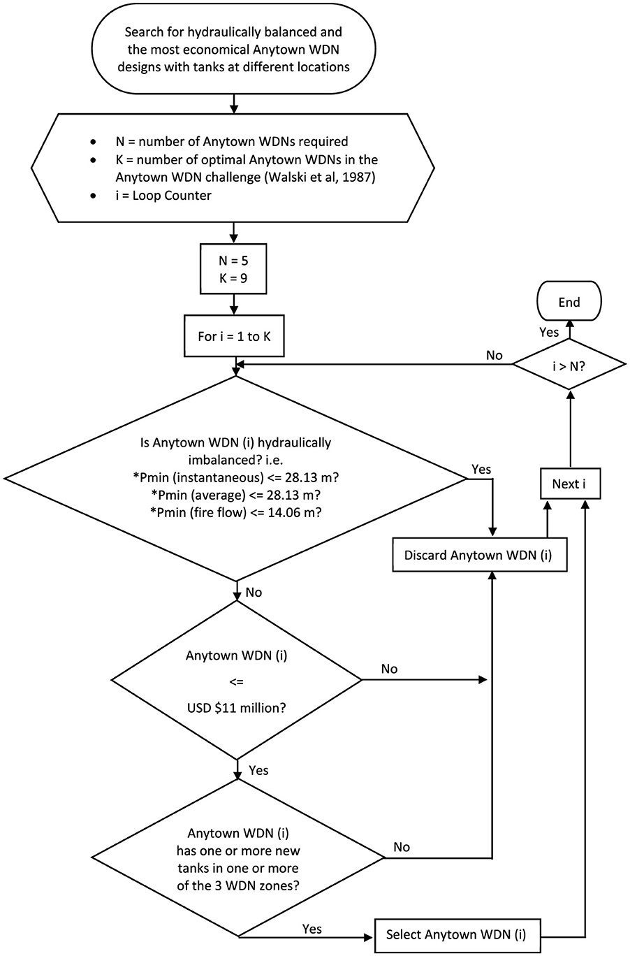
Figure 3. Algorithm for determining optimal ATN designs with tanks at different locations.

Prior to the “Battle”, the ATN had 2 tanks—the 1st was located at node 41 and the 2nd was located at node 42. These tanks were inadequate for the anticipated growth in the Anytown community and additional tanks were recommended during the “Battle” to cater for future demands (Walski et al., 1987).

Some of the optimal ATN designs that satisfied the conditions for hydraulic balance and cost ≤ $11 million were Walters et al. (1999) Design 1, Vamvakeridou-Lyroudia et al. (2007); Prasad (2010) Case 2 Design, Siew et al. (2016) Design 1, and Siew et al. (2016) Design 2. These designs, which were employed in phases (ii) and (iv), are described in summary below and recommend additional tanks at nodes shown on Figure 1.

• The Walters et al. (1999) Design 1 (W) cost $10.91 million and recommended 2 additional tanks—the 1st was located at node 5 and the 2nd was located at node 12.

• The Vamvakeridou-Lyroudia et al. (2007) Design (V) cost $10.74 million and recommended 2 additional tanks—the 1st was located at node 9 and the 2nd was located at node 16.

• The Prasad (2010) Case 2 Design (P) cost $10.59 million and recommended 2 additional tanks—the 1st was located at node 9 and the 2nd was located at node 16.

• The Siew et al. (2016) Design 1 (S1) cost $10.31 million and recommended 1 additional tank to be located at node 7.

• The Siew et al. (2016) Design 2 (S2) cost $10.41 million and recommended 1 additional tank to be located at node 6.

2.2 Phase (ii) and phase (iii)

To undertake a reliability assessment of a WDN, that WDN must first be hydraulically balanced. In phase (ii), EPANET 2.2 (Rossman, 2000) was employed to hydraulically simulate, using pressure driven analysis, the five optimal ATN designs obtained in phase (i). Validation of the simulation results obtained was achieved when these results were compared with the results published in the literature for each ATN design.

Simulation results generated by EPANET were then input into the Microsoft Excel^® tool that was developed in phase (iii) to generate hydraulic reliability and failure tolerance values based on the methodology employed in Tanyimboh's (1993) PRAAWDS tool. PRAAWDS is abbreviation for: Programme for the Realistic Analysis of the Availability of Water in Distribution Systems. PRAAWDS was applied to the SN. Validation of the Microsoft Excel^® tool was achieved by comparing the hydraulic reliability and failure tolerance values calculated for designs 1, 3, and 12 of the SN (Tanyimboh and Templeman, 2000; Tanyimboh and Setiadi, 2008) with the results obtained by the Microsoft Excel^® tool for the same SN designs. The SN designs (1, 3, and 12) were selected because their reliability values were sensitive to layout changes and this was ideal for this study since any layout changes to a network (i.e., different tank locations) should reflect the extent to which reliability is affected.

Well-known techniques for assessing the reliability of WDNs include robust techniques (Tanyimboh, 1993), surrogate techniques (Tanyimboh and Templeman, 1995) and probabilistic techniques (Wagner et al., 1988). Surrogate techniques are empirical equations that can be used to assess the performance of WDNs. However, they are not as sturdy as robust techniques, which are the basis for pressure driven analysis (Tanyimboh and Templeman, 1995). Probabilistic techniques are generally more accurate than surrogate and robust techniques since they account for the random behavior of WDNs. However, they can be time-consuming since they require historical data, which may not always be available. In this study, robust techniques (specifically hydraulic reliability equations) were employed.

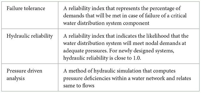
According to Tanyimboh (1993), hydraulic reliability, R (Equation 1) deals with the state of a system. For instance, a system with more pipe loops, tanks or pumps would have a higher hydraulic reliability (close to unity) than a system that does not have these.

$\begin{array}{l}\text{R}=\frac{1}{\text{T}}\left(\text{p}(0)\text{T}(0)+{\displaystyle \sum _{\text{m}=1}^{\text{M}}}\text{p}(\text{m})\text{T}(\text{m})+{\displaystyle \sum _{\begin{array}{c}m=1\\ \forall \text{n}>m\\ \end{array}}^{\text{M}-1}}\text{p}(\text{m},\text{n})\text{T}(\text{m},\text{n})+\dots \right)\\ +\frac{1}{2}\left(1-\text{p}(0)-{\displaystyle \sum _{\text{m}=1}^{\text{M}}}\text{p}(\text{m})-{\displaystyle \sum _{\begin{array}{c}m=1\\ \forall \text{n}>m\\ \end{array}}^{\text{M}-1}}\text{p}(\text{m},\text{n})-\dots \right)& (1)\end{array}$

Similarly, failure tolerance, FT (Equation 2; Tanyimboh, 1993) measures a system's performance when one or more of the WDN's components (pipe loops, tanks or pumps) are unavailable or non-functional. Thus, failure tolerance estimates the portion of total demand that will be met when one or more system components are unavailable. Networks with failure tolerance values between 0.60 and 1.00 are considered less vulnerable (Tanyimboh et al., 2016).

$\begin{array}{ll}\text{F}\text{T}=\frac{\text{R}-\frac{\text{p}(0)\text{T}(0)}{\text{T}}}{1-\text{p}(0)}& (2)\end{array}$

Equations 3–6 (Tanyimboh, 1993) and Equation 7 (the mechanical availability equation by Cullinane et al., 1992) are employed in the computation of Equations 1 and 2:

$\begin{array}{ll}\text{p}(0)={\displaystyle \prod _{\text{m}=1}^{\text{M}}}{\text{a}}_{\text{m}}={\text{a}}_1\times {\text{a}}_2\times {\text{a}}_3\times \dots & (3)\end{array}$

$\begin{array}{ll}{\text{u}}_{\text{m}}=1-{\text{a}}_{\text{m}}& (4)\end{array}$

$\begin{array}{ll}\text{p}(\text{m})=\text{p}(0)(\frac{{\text{u}}_{\text{m}}}{{\text{a}}_{\text{m}}}),\text{f}\text{o}\text{r}\text{a}\text{s}\text{i}\text{n}\text{g}\text{l}\text{e}\text{p}\text{i}\text{p}\text{e}\text{f}\text{a}\text{i}\text{l}\text{u}\text{r}\text{e}& (5)\end{array}$

$\begin{array}{ll}\text{p}(\text{m},\text{n})=\text{p}(0)\left(\frac{{\text{u}}_{\text{m}}}{{\text{a}}_{\text{m}}}\right)\times (\frac{{\text{u}}_{\text{n}}}{{\text{a}}_{\text{n}}}),\text{f}\text{o}\text{r}\text{t}\text{w}\text{o}\text{p}\text{i}\text{p}\text{e}\text{s}\text{f}\text{a}\text{i}\text{l}\text{u}\text{r}\text{e}& (6)\end{array}$

$\begin{array}{ll}{\text{a}}_{\text{m}}=\frac{0.21218{\text{d}}^{1.462131}}{0.00074{\text{d}}^{0.285}+0.21218{\text{d}}^{1.462131}}& (7)\end{array}$

where:

• R is hydraulic reliability with values between 0 and 1.

• M is number of links (pipes, pumps, and valves).

• p(0) is probability that all pipes are operational.

• a_m is the probability that pipe m is operational.

• p(m) is the probability that only pipe m is not operational.

• u_m is a probability that pipe m is not operational.

• P(m, n) is the probability that only pipes m and n are not operational.

• T(0) is the total flow (l/s) supplied at adequate pressure when all pipes are operational.

• T(m) is the total flow (l/s) supplied when only pipe m is not operational.

• T(m, n) is the total flow (l/s) supplied when only pipes m and n are not operational.

• T is the sum of the nodal demands in l/s.

• FT is failure tolerance with values between 0 and 1.

• d is pipe diameter (mm).

2.3 Phase (iv)

Phase (iv) involved computing the hydraulic reliabilities and failure tolerances of the different optimal ATN designs obtained in phase (i). As shown in Figure 1, there are three zones where tanks may be located during WDN design i.e.,: upstream of the demand center (the zone where the booster station is typically located), the demand center and downstream of the demand center.

To simulate pipe failure, certain functional pipes were closed during hydraulic simulation. The selection of pipe for failure was based on the risk of failure, which was obtained using Equation 5. Tanyimboh and Templeman (1995) recommended that several scenarios, which may give rise to unreliability, should be considered to accurately compare designs in terms of failure tolerance. In phase (iv), three scenarios were compared i.e., failure of any pipe; failure of the transmission mains pipe between the source node and node 1 (see Figure 2); and failure of pipes with the smallest diameters and therefore, the highest failure probabilities. The 3rd scenario was the most realistic and therefore, the single pipes that were closed during failure tolerance analysis were smaller diameter pipes. It is uncommon in the operation of WDNs that two or more pipes or components fail at the same time (Shuang et al., 2014).

Hydraulic reliability and failure tolerance analysis were conducted under steady-state conditions, which is best suited for speedily analyzing networks under the worst-case operational scenario (i.e., peak demand). This approach was similarly employed in previous reliability assessment studies (Tanyimboh and Templeman, 2000; Tanyimboh, 2003 and Tanyimboh and Setiadi, 2008).

3 Results and discussion

3.1 Comparison of phase (ii) results for the optimal ATN designs selected in phase (i)

Table 1 presents the results of the EPANET 2.2 hydraulic simulation of the optimal ATN designs identified in phase (i), alongside the results published by the various authors. The table shows that the EPANET 2.2 results are identical to the published results for each of the designs. Similar to the comparison of node pressures in Table 1, the variation in tank water levels were compared. For example, the extended period simulation of tank water levels in the old tanks at nodes 41 and 42 of Figure 4B (this study) correspond to water levels in the same tanks at nodes 65 and 165 in Figure 4A (Vamvakeridou-Lyroudia et al., 2007) respectively.

Table 1

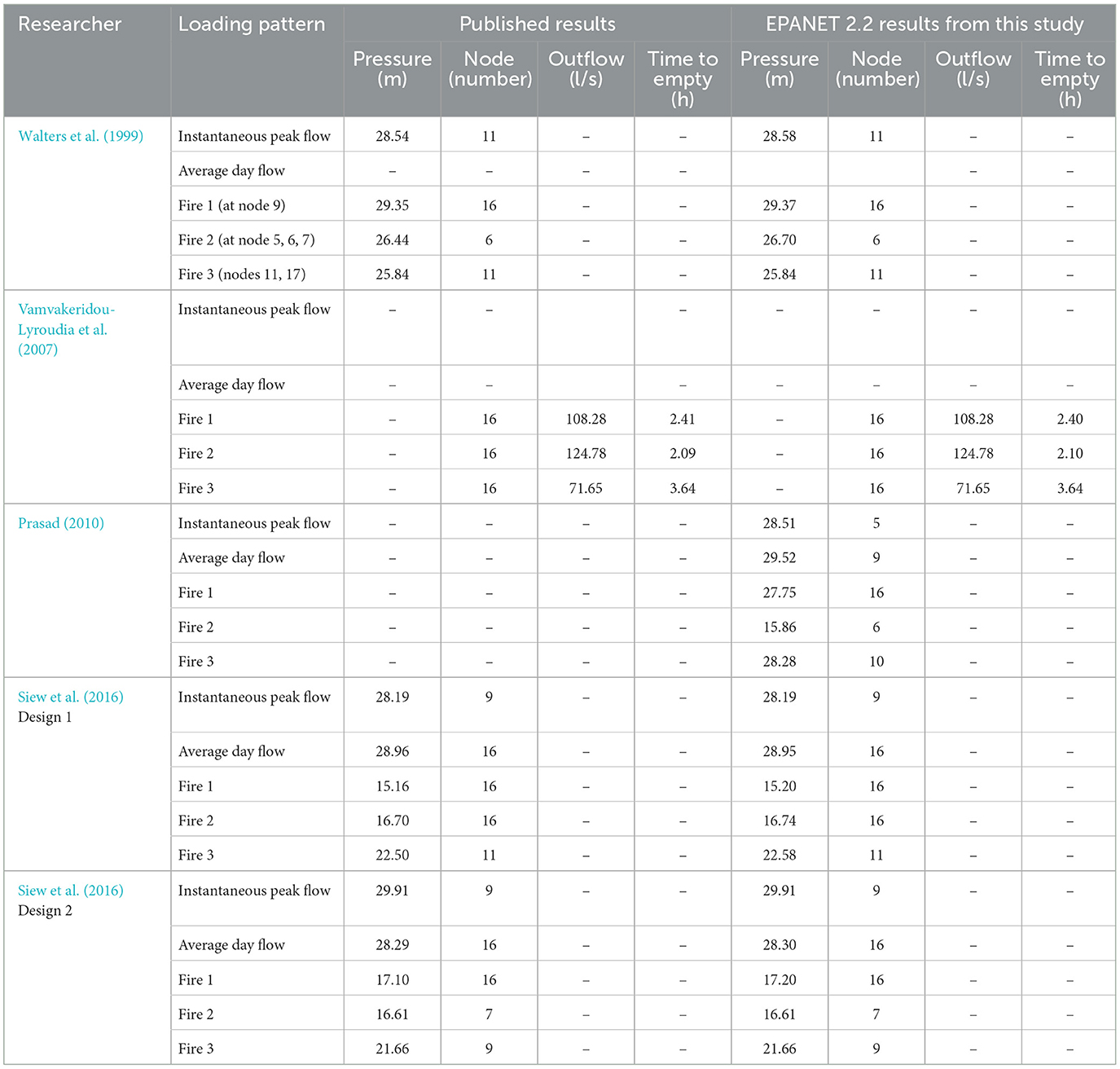
Table 1. Comparison of hydraulic simulated results for the optimal ATN designs.

Figure 4

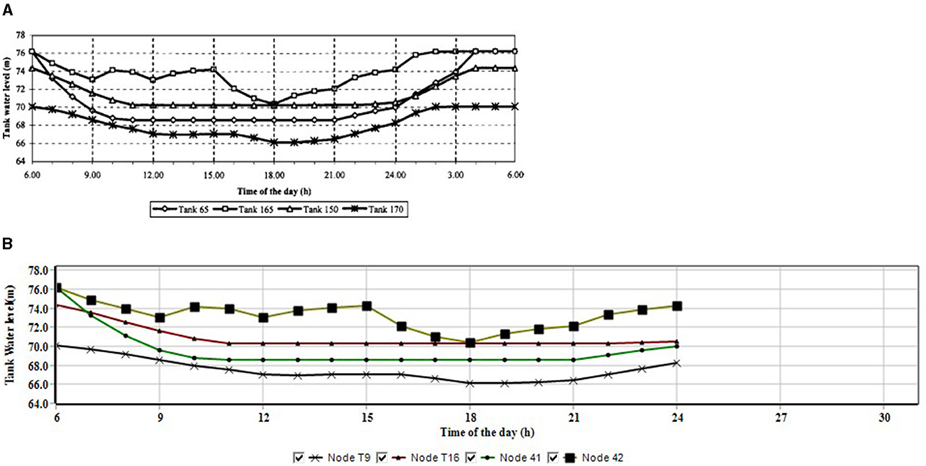
Figure 4. (A) Variation of tank water levels in the ATN (Vamvakeridou-Lyroudia et al., 2007). (B) Variation of tank water levels in the ATN (this study).

3.2 Validation of the Microsoft Excel^® tool developed in phase (iii)

Table 2 compares the hydraulic reliability (Equation 1) and failure tolerance (Equation 2) results calculated by Tanyimboh and Setiadi (2008) for the SN with those calculated using the MS Excel^® tool developed in phase (iii).

Table 2

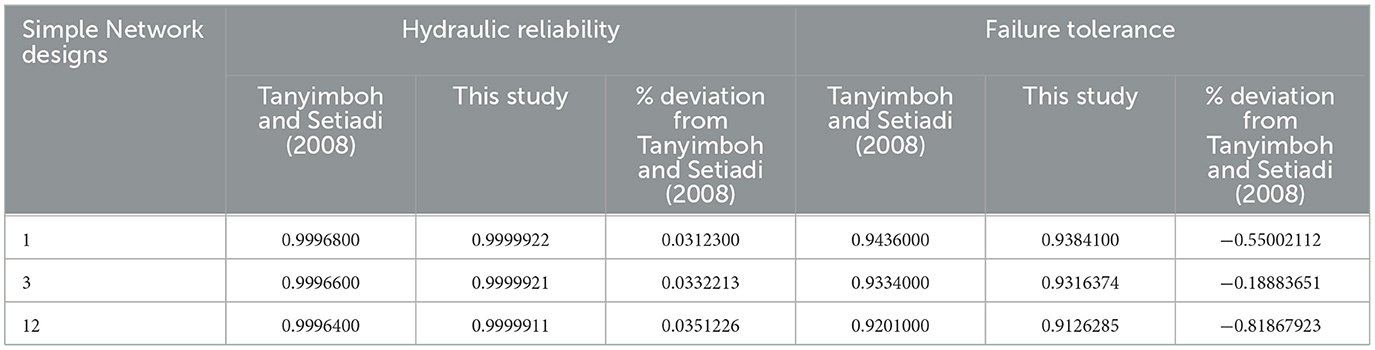
Table 2. Comparison of hydraulic reliability and failure tolerance results for the Simple Network.

As can be seen, there are insignificant differences (< ±1%) between the hydraulic reliability and failure tolerance results obtained by Tanyimboh and Setiadi (2008) and those obtained in phase (iv). The differences are likely because the two studies selected different pipes for closure during failure simulations—Tanyimboh and Setiadi (2008) did not specify the pipes they employed in their failure analysis and whether single or multiple pipes were closed during analysis. The results for hydraulic reliability and failure tolerance generated in phase (iv) were therefore ~99% similar to the results obtained by Tanyimboh and Setiadi (2008) and therefore validate the developed Microsoft Excel^® tool's capability to calculate hydraulic reliability and failure tolerance.

3.3 Calculation of hydraulic reliabilities and failure tolerances for the optimal ATN designs (phase iv)

Table 3 presents the hydraulic reliability and failure tolerance results for the optimal ATN designs using the Microsoft Excel^® tool developed in phase (iii). All the optimal ATN designs obtained hydraulic reliabilities close to 1.0—this result was expected since each ATN design was optimal (Tanyimboh and Templeman, 1995).

Table 3

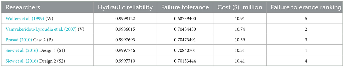
Table 3. Hydraulic reliability and failure tolerance results for the optimal ATN designs.

The best location for the additional tank(s) that each optimal ATN design proposed was thereafter assessed using failure tolerance. The different locations of the tanks were expected to influence each designs' response to pipe failure and therefore, generate different failure tolerance values. The highest failure tolerance value represents the best location. The list below summarizes results from this phase (see Table 3):

• All the optimal ATN designs generated a failure tolerance value higher than 0.68. The implication of this is that in the event of a distribution mains pipe failure, tanks in each design would ensure uninterrupted supply to more than 68% of consumers, at the specified design flows and pressures.

• The Walters et al. (1999) design, which recommended 2 additional tanks (the 1st was located downstream of the demand center and the 2nd was located upstream of the demand center) generated the least failure tolerance value of 0.6874 and was the most expensive of the designs.

• A failure tolerance of 0.7043 was calculated for the Vamvakeridou-Lyroudia et al. (2007) design, which recommended 2 additional tanks (the 1st was located downstream of the demand center and the 2nd was located at the demand center). When compared with the Walters et al. (1999) design, failure tolerance was improved because the 2nd tank was located at the demand center. The Prasad (2010) design also recommended 2 additional tanks at the same nodes as the Vamvakeridou-Lyroudia et al. (2007) design and not surprisingly, generated a similar failure tolerance value.

• The Siew et al. (2016) Design 1 generated the highest failure tolerance with one additional tank recommended for downstream of the demand center. The Siew et al. (2016) Design 1 was the cheapest design. This result therefore shows that a more reliable design need not be the most expensive design and that the best location for the additional tank(s) in the ATN is downstream of the demand center.

• It is immaterial that the failure tolerance values were closely clustered, ranging between 0.6874 and 0.7084, because the designs were optimal. In practice however, similar or different results may be obtained depending on the optimality of the WDN design. In terms of the best location for tanks in the WDN, what is material is identifying the design that produces the highest failure tolerance.

4 Conclusion

This study developed a tool in Microsoft Excel^® to compute failure tolerance when pipe failure occurs in a WDN, and as a consequence, determines the optimal location of a tank(s). The highest failure tolerance value among several designs of the WDN, with tanks at different locations, produces the best location. For the Anytown Network, the design with a tank located downstream of the demand center proved to be the best location. The incorporation of hydraulic reliability and failure tolerance calculations into EPANET (as well as other hydraulic simulation software) would certainly be beneficial for determining, during design, the best location(s) for tanks within networks and computationally, would be more efficient than was the case in this study.

Data availability statement

The original contributions presented in the study are included in the article/supplementary material, further inquiries can be directed to the corresponding author.

Author contributions

AK: Methodology, Formal analysis, Investigation, Software, Validation, Writing – original draft. AI: Methodology, Supervision, Writing – review & editing.

Funding

The author(s) declare that no financial support was received for the research, authorship, and/or publication of this article.

Acknowledgments

The authors would like to thank Professor Tiku Tanyimboh for inspiring this research project and his supervision efforts at the beginning.

Conflict of interest

The authors declare that the research was conducted in the absence of any commercial or financial relationships that could be construed as a potential conflict of interest.

Publisher's note

All claims expressed in this article are solely those of the authors and do not necessarily represent those of their affiliated organizations, or those of the publisher, the editors and the reviewers. Any product that may be evaluated in this article, or claim that may be made by its manufacturer, is not guaranteed or endorsed by the publisher.

References

Abunada, M., Trifunović, N., Kennedy, M., and Babel, M. (2014). Optimization and reliability assessment of water distribution networks incorporating demand balancing tanks. Proc. Eng. 70, 4–13. doi: 10.1016/j.proeng.2014.02.002

Crossref Full Text | Google Scholar

Ajitha, T. T., and Viji, R. (2023). Site suitability analysis of water tank in Athivilai village of India using an analytical hierarchy process and a geographical information system. Water Supply 23, 3805–3818. doi: 10.2166/ws.2023.222

Crossref Full Text | Google Scholar

Basile, N., Fuamba, M., and Barbeau, B. (2008). “Optimization of water tank design and location in water distribution systems,” in Proceedings of the 10th Annual Water Distribution Systems Analysis, eds. J. E. van Zyl, A. Ilemobade, and H. E. Jacob, 361–373. doi: 10.1061/41024(340)32

Crossref Full Text | Google Scholar

Cullinane, M. J., Lansey, K. E., and Mays, L. W. (1992). Optimization-availability-based design of water distribution networks. J. Hyd. Eng. 118, 420–441. doi: 10.1061/(ASCE)0733-9429(1992)118:3(420)

Crossref Full Text | Google Scholar

Curtin, B. (2024). Optimizing Storage Tank Design for Efficient Potable Water Supply (Doctoral dissertation). Worcester Polytechnic Institute. Available at: https://digital.wpi.edu/concern/student_works/gb19f972v?locale=pt-BR (accessed October 5, 2024).

Google Scholar

Darweesh, M. S. (2021). Elevated tanks effect on transient pressures: case study. J. Water Sanit. Hyg. Dev. 11, 629–637. doi: 10.2166/washdev.2021.022

Crossref Full Text | Google Scholar

Farmani, R., Walters, G. A., and Savic, D. A. (2005). Trade-off between total cost and reliability for Anytown water distribution network. J. Water Resour. Plann. Manag. 161–171. doi: 10.1061/(ASCE)0733-9496(2005)131:3(161)

Crossref Full Text | Google Scholar

Ilemobade, A. A., and Stephenson, D. (2006). Application of a constrained non-linear hydraulic gradient design tool to water reticulation network upgrade. Urban Water J. 3, 199–214. doi: 10.1080/15730620601060213

Crossref Full Text | Google Scholar

Mabrok, M. A., Saad, A., Ahmed, T., and Alsayab, H. (2022). Modeling and simulations of Water Network Distribution to Assess Water Quality: Kuwait as a case study. Alexand. Eng. J. 61, 11859–11877. doi: 10.1016/j.aej.2022.05.038

Crossref Full Text | Google Scholar

Marlim, M. S., and Kang, D. (2023). Energy intensity-based metric for optimal design of water distribution systems. Appl. Water Sci. 13:185. doi: 10.1007/s13201-023-01998-z

Crossref Full Text | Google Scholar

Murphy, L. J., Dandy, G. C., and Simpson, A. R. (1994). “Optimum design and operation of pumped water distribution systems,” in Conference on Hydraulics in Civil Engineering, 2–13. Available at: https://www.researchgate.net/profile/Angus-Simpson/publication/256097672_Optimum_Design_and_Operation_of_Pumped_Water_Distribution_Systems/links/02e7e521c1ed3a650a000000/Optimum-Design-and-Operation-of-Pumped-Water-Distribution-Systems.pdf

Google Scholar

Prasad, T. D. (2010). Design of pumped water distribution networks with storage. J. Water Resour. Plann. Manag. 136, 129–132. doi: 10.1061/(ASCE)0733-9496(2010)136:1(129)

Crossref Full Text | Google Scholar

Rossman, L. A. (2000). EPANET 2: User's Manual. Available at: https://www.microimages.com/documentation/tutorials/epanet2usermanual.pdf (accessed March 3, 2022).

Google Scholar

Saldarriaga, J., Bohorquez, J., Celeita, D., Vega, L., Paez, D., Savic, D., et al. (2019). Battle of the water networks district metered areas. J. Water Resour. Plann. Manag. 145:04019002. doi: 10.1061/(ASCE)WR.1943-5452.0001035

PubMed Abstract | Crossref Full Text | Google Scholar

Seyoum, A. G., Tanyimboh, T. T., and Siew, C. (2014). “Optimal tank design and operation strategy to enhance water quality in distribution systems,” in Proceedings: 11th International Conference on Hydroinformatics (New York, NY: City University of New York (CUNY) Academic Works), 1–14. Available at: https://academicworks.cuny.edu/cc_conf_hic/324Discoveradditionalworksat:https://academcworks.cuny.edu (accessed March 3, 2023).

Google Scholar

Shuang, Q., Zhang, M., and Yuan, Y. (2014). Performance and reliability analysis of water distribution systems under cascading failures and the identification of crucial pipes. PLoS ONE 9:e88445. doi: 10.1371/journal.pone.0088445

PubMed Abstract | Crossref Full Text | Google Scholar

Siew, C., Tanyimboh, T. T., and Seyoum, A. G. (2016). Penalty-free multi-objective evolutionary approach to optimization of anytown water distribution network. Water Resour. Manag. 30, 3671–3688. doi: 10.1007/s11269-016-1371-1

Crossref Full Text | Google Scholar

Singh, M. K., and Kekatos, V. (2019). Optimal scheduling of water distribution systems. IEEE Transact. Control Netw. Syst. 7, 711–723. doi: 10.1109/TCNS.2019.2939651

Crossref Full Text | Google Scholar

Spedaletti, S., Rossi, M., Comodi, G., Salvi, D., and Renzi, M. (2021). Energy recovery in gravity adduction pipelines of a water supply system (WSS) for urban areas using Pumps-as-Turbines (PaTs). Sustain. Energy Technol. Assess. 45:101040. doi: 10.1016/j.seta.2021.101040

Crossref Full Text | Google Scholar

Tanyimboh, T. (2003). “Reliability analysis of water distribution systems,” in Proceedings of the 30th IAHR Congress. Urban and Rural Water Systems for Sustainable Development, eds. J. Ganoulis, C. Maksimovic, and V. Kaleris (Thessaloniki: AuTH), 321–328. Available at: https://www.iahr.org/library/infor?pid=25334 (accessed February 8, 2023).

Google Scholar

Tanyimboh, T. T., and Templeman, A. B. (1995). “A new method for calculating the reliability of single-source networks,” in Developments in Computational Techniques for Civil Engineering, ed. B. H. V. Topping (Edinburgh: Civil-Comp Press), 1–9. doi: 10.4203/ccp.32.1.1

PubMed Abstract | Crossref Full Text | Google Scholar

Tanyimboh, T. T. (1993). An Entropy-Based Approach to the Optimum Design of Reliable Water Distribution Networks (Ph.D. thesis). University of Liverpool. doi: 10.17638/03175136

PubMed Abstract | Crossref Full Text | Google Scholar

Tanyimboh, T. T., and Setiadi, Y. (2008). Joint layout, pipe size and hydraulic reliability optimization of water distribution systems. Eng. Optimiz. 40, 729–747. doi: 10.1080/03052150802046353

Crossref Full Text | Google Scholar

Tanyimboh, T. T., Siew, C., Saleh, S., and Czajkowska, A. (2016). Comparison of surrogate measures for the reliability and redundancy of water distribution systems. Water Resour. Manag. 30, 3535–3552. doi: 10.1007/s11269-016-1369-8

Crossref Full Text | Google Scholar

Tanyimboh, T. T., and Templeman, A. B. (2000). Quantified assessment of the relationship between the reliability and entropy of water distribution systems. Eng. Optimiz. 33, 179–199. doi: 10.1080/03052150008940916

PubMed Abstract | Crossref Full Text | Google Scholar

Torkomany, M. R., Yusuf, M. M., Elkholy, M., Abdelrazek, A. M., and Fath, H. E. S. (2020). “Optimum reliable design of water distribution systems using particle swarm optimization considering pumping power and tank siting,” in 2020 Advances in Science and Engineering Technology International Conferences (ASET). doi: 10.1109/ASET48392.2020.9118336

Crossref Full Text | Google Scholar

Vamvakeridou-Lyroudia, L. S., Savic, D. A., and Walters, G. A. (2007). tank simulation for the optimization of water distribution networks. J. Hyd. Eng. 133, 625–636. doi: 10.1061/(ASCE)0733-9429(2007)133:6(625)

PubMed Abstract | Crossref Full Text | Google Scholar

van Dijk, M., van Vuuren, S. J., and van Zyl, J. E. (2008). Optimising water distribution systems using a weighted penalty in a genetic algorithm. Water SA 34:180651. doi: 10.4314/wsa.v34i5.180651

Crossref Full Text | Google Scholar

van Zyl, J. E. (2014). Introduction to Operation and Maintenance of Water Distribution Systems. Water Research Commission of South Africa. Available at: https://www.pseau.org/outils/ouvrages/wrc_introduction_to_operation_and_maintenance_of_water_distribution_systems_2014.pdf

Google Scholar

van Zyl, J. E., Asce, M., Piller, O., and le Gat, Y. (2008). Sizing municipal storage tanks based on reliability criteria. J. Water Resour. Plann. Manag. 134, 548–555. doi: 10.1061/(ASCE)0733-9496(2008)134:6(548)

Crossref Full Text | Google Scholar

Wagner, J. M., Shamir, U., and Marks, D. H. (1988). Water distribution reliability: analytical methods. J. Water Resour. Plann. Manage. 114, 253–275. doi: 10.1061/(ASCE)0733-9496(1988)114:3(253)

Crossref Full Text | Google Scholar

Walski, T. M., Downey Brill, E. Jr., Gessler, J., Goulter, I. C., Jeppson, R. M., et al. (1987). Battle of the network models: epilogue. J. Water Resour. Plann. Manag. 113, 191–203. doi: 10.1061/(ASCE)0733-9496(1987)113:2(191)

Crossref Full Text | Google Scholar

Walters, G. A., Halhal, D., Savic, D., and Ouazar, D. (1999). Improved design of “Anytown” distribution network using structured messy genetic algorithms. Urban Water 1, 23–38. doi: 10.1016/S1462-0758(99)00005-9

Crossref Full Text | Google Scholar

Glossary