Advancing non-optical water quality monitoring in Lake Tana, Ethiopia: insights from machine learning and remote sensing techniques

Water quality is deteriorating in the world's freshwater bodies, and Lake Tana in Ethiopia is becoming unpleasant to biodiversity. The objective of this study is to retrieve non-optical water quality data, specifically total nitrogen (TN) and total phosphorus (TP) concentrations, in Lake Tana using Machine Learning (ML) techniques applied to Landsat 8 OLI imagery. The ML methods employed include Artificial Neural Networks (ANN), Support Vector Regression (SVR), Random Forest Regression (RF), XGBoost Regression (XGB), AdaBoost Regression (AB), and Gradient Boosting Regression (GB). The XGB algorithm provided the best result for TN retrieval, with determination coefficient (R²), mean absolute error (MARE), relative mean square error (RMSE) and Nash Sutcliff (NS) values of 0.80, 0.043, 0.52, and 0.81 mg/L, respectively. The RF algorithm was most effective for TP retrieval, with R² of 0.73, MARE of 0.076, RMSE of 0.17 mg/L, and NS index of 0.74. These methods accurately predicted TN and TP spatial concentrations, identifying hotspots along river inlets and northeasters. The temporal patterns of TN, TP, and their ratios were also accurately represented by combining in-situ, RS and ML-based models. Our findings suggest that this approach can significantly improve the accuracy of water quality retrieval in large inland lakes and lead to the development of potential water quality digital services.

1 Introduction

Of the largest freshwater resources, the African continent hosts the Nile and the Congo River (Laraque et al., 2020) and three of the 10 largest freshwater lakes, namely Victoria, Tanganyika and Malawi lakes (Hastie et al., 2021). The 21st century's global challenge of ensuring water quality is escalating due to the growing global freshwater crisis. The combined effect of climate change, environmental alterations, and anthropogenic pressures has threatened freshwater availability in terms of quantity and quality in Africa. It has become one of the major concerns, yet it remains one of the least studied.

Eutrophication, mainly caused by anthropogenic activities of freshwater water ecosystems has consequences that include changes in phytoplankton species composition and increase in bio-volume that are accompanied by oxygen depletion, decreases in water transparency, and loss of biodiversity (Bunting et al., 2005). Phosphorus has long been identified as the ultimate limiting nutrient attributed as the main driver of eutrophication when received in excess within freshwater ecosystems. Most previous management strategies to reverse eutrophication have been based on asserting that P is the limiting nutrient in most freshwater ecosystems (Schindler, 2012). However, there is growing evidence of N limitation (Bunting et al., 2005) or NP co-limitation (Sterner, 2008) of primary production within various freshwater ecosystems. A similar phenomenon in Lake Tana, where the lake has been shifting from P-limited to N-limited, was observed (Dersseh et al., 2022). Consequently, the lake is at risk with strong evidence that its ecological health is highly toxic for invertebrates and fish from agricultural inputs (Sishu et al., 2022).

Thus, continuous monitoring of water bodies' nutrients and the nutrient-limited condition of the water bodies are essential to devising an appropriate management strategy for the protecting the lake and other water bodies in Africa. However, long-term continuous water quality monitoring in most African inland waterbodies is lacking due to limited monitoring infrastructure, financial constraints, and limited technical capacity. In these regards, it is crucial to look for an alternative approach for monitoring water quality parameters, such as non-optically active water quality parameters (TN and TP concentrations) of waterbodies. Remote Sensing (RS) based monitoring allows for the routing of broad regions in a short amount of time and on a representative basis and is a cost-effective method of water quality monitoring (Zhang H. et al., 2022).

Current methods for estimating water quality parameters from Remote Sensing (RS) mainly include physical and empirical models. However, these methods make it difficult to solve the complex non-linear relationship between the water quality parameters and the spectral indices of RS data (Lan et al., 2023). Machine learning (ML) algorithms on the contrary have become a best option for retrieving water quality parameters in the inland lake (Cao et al., 2020; Bygate and Ahmed, 2024; Tesfaye, 2024). The premises to retrieve TN and TP from RS images have been based on the strong correlation that these non-optical parameters have shown with optically active substances (Guo et al., 2020; Sagan et al., 2020). Moreover, studies indicated that RS integrated with Machine Learning (ML) has been used successfully to monitor these water quality parameters in various scales and areas.

A TP concentration prediction in a macrophytic lake with a spectral characteristic dominated by chlorophyll Lake Baiyangdian showed a high performance using the partial least square (PLS) regression model (Zhang L. et al., 2022). A similar study of ML models for TP and TN concentration inversion using measured data and satellite imagery band reflectance, in Dongting Lake, china, showed the established empirical model can accurately estimate TP (Zhang Y. et al., 2022). Guo et al. (2020) on the other hand developed an ML-based water-quality monitoring method for total phosphorous (TP), total nitrogen (TN), and chemical oxygen demand (COD) for small urban waterbodies from the recently launched Sentinel-2. The retrieval performances of these non-optically active parameters were significantly improved by the optimized machine-learning models and imagery band selections. The choice of the algorithms largely depends on the modeling capacity of the algorithm to capture complex phenomena of the water quality processes, the data availability, the spatio-temporal representation of the data used, the frequency of data and others (Guo et al., 2020; Zhang L. et al., 2022; Zhang Y. et al., 2022). Furthermore, the satellite satellite depends on the spatial and temporal resolution requirement, availability of extended data used for trend analysis, and the size of the water body under investigation.

There is an urgent need to monitor the nutrient status of the freshwater, and making it critical to evaluate the effectiveness of the methods for retrieval of non-optical water quality parameters such as TN and TP concentrations in Africa particularly in the study area. Recently, ML-based RS retrieval approach was applied for Lake Tana to retrieve an optically active water quality parameters: chlorophyll, turbidity, and transparency, and it had worked reasonably well (Leggesse et al., 2023). Accordingly, this study suggested Random Forest Regression (RF), Adaboost Regression (AB), Gradient boost regression (GB), support vector regression (SVR), Extreme gradient boosting regression (XGB) and ANN algorithms to retrieve non-optically active parameters from Landsat 8 OLI imagery for Lake Tana. Most suggested ML algorithms were ensemble learning algorithms that could not only obtain a better fitting search space, but also reduces the risk of overfitting (Sagi and Rokach, 2018; Leggesse et al., 2023).

The ML method to retrieve non-optically active parameters (TN and TP) from remotely sensed data was based on the correlation of in situ measurement of TN and TP concentrations with the bands available in the satellites and derived spectral indices. Point-based TN and TP concentrations measurements were used for some of the months between 2016–2022. Google Earth Engine (GEE), a cloud computing platform was used to extract the primary bands of Landsat 8 OLI for the corresponding sampling points. In addition, a large set of spectral indices were calculated to provide the ML algorithms and Recursive Feature Elimination with Cross Validation (RFECV) technique (Kim et al., 2014) was employed to select the optimum features. Due to the limited field-based water quality samples, k-fold cross validation approached was used to improve the ML algorithms performance (Wieczorek and Guerin, 2022).

The study further evaluated the spatiotemporal variations and influencing factors of TN and TP concentrations to provide scientific references for preventing the pollution and eutrophication of Lake Tana and other water bodies.

2 Materials and methods

2.1 Study area

Lake Tana is situated at an elevation of 1,786 m above sea level (Figure 1) and has a surface area of ~3,050 km² during the dry season and 3,600 km² toward the end of the rainy season. Its drainage basin covers an area of 15,054 km², lying between 10°56′ and 12°45′ north latitude and 36°44′ to 38°14′ east longitude. The Lake surface area accounts for 20% of the drainage area. The United Nations Educational, Scientific and Cultural Organization (UNESCO) has designated the lake as a biosphere reserve (Vijverberg et al., 2009). The climate around the lake is a warm-temperate tropical highland monsoon with high diurnal temperature variation between daytime extremes of 30°C and nighttime lows of 6°C, a mean temperature of 21.7°C, significant diurnal but small seasonal changes of 5°C, and two temperature peaks around May/June and October/November.

Figure 1

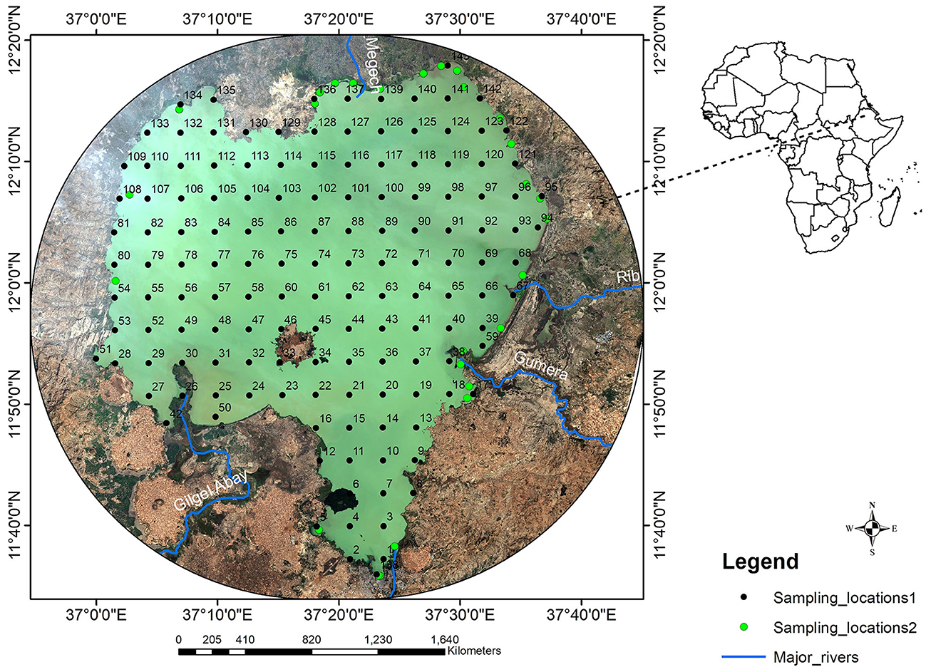
Figure 1. Study area and the sampling locations; sampling location 1 indicate the 143 sampling locations and sampling location 2 indicates the 27 sampling points.

It is a dry season between November and May, while between June and October, it is a distinct rainy season (kiremt) (Wondie and Mengistou, 2014). The average annual rainfall in the Lake is 1,355 mm. Over 60 rivers and streams feed Lake Tana. The main tributary rivers are Gilgel Abay, Gumera, Ribb, Gelda, Megech, and Dirma. According to Taye et al. (2021), the dominant land use of the basin was cultivated land which accounts for 67% of the drainage basin. The second dominant land cover was the lake surface area with coverage of 20.5%, and the third dominant is the forest area, which covers 4.8%. The remaining 7.3% of the drainage basin is covered by grassland, shrubs, built-up and bare land. The lake also receives urban runoff and domestic waste effluents from the three major cities of Bahir Dar, Gonder, and Debre Tabor (Abera et al., 2021).

2.2 Water samples collection and laboratory analysis

A monthly dataset of two non-optically active water quality parameters, TN and TP concentrations of the lake, was obtained both from Dersseh et al. (2019) for the years before 2020 and from primary data collection in the years 2021 and 2022. The dataset was collected from 170 sampling locations across the lake at a 5 km resolution from the top water surface at a depth of 50 cm in the months of August 2016, December 2016, March 2017 and from 143 sampling locations in the months of October 2021, April 2022 and October 2022 (Figure 1: sampling_locations1) and data collected from 27 sampling locations in June 2019, July 2019, August 2019, September 2019, December 2019, and March 2020 (Figure 1: sampling_locations2). For each of the two water quality variables, there were 1,101 data points during the seven years. The sampling dates for both TN and TP concentration were chosen to represent the primary rainy season (July–September), the dry season (December–April), and the pre-rainy season (May–June) to understand how seasonality influences the water quality parameters.

The water quality parameters were analyzed in the Bahir Dar Institute of Technology water quality laboratory. The TP concentration was determined based on ammonium molybdate spectrophotometry. The oxidant potassium persulfate was added to the water sample, and the phosphorus in the water sample was oxidized to orthophosphate at a temperature of 120°C. Then, sodium hydroxide solution was added to the cooled water sample to adjust it to neutrality, and finally, ascorbic acid and molybdic acid solution were added and mixed thoroughly. After the complete reaction, a blue complex was formed, and the absorbance was measured with a spectrophotometer at a 700 nm wave-length. The concentration of TP was calculated by comparing experiments with blank water samples.

The TN concentration was determined using an alkaline potassium persulfate digestion ultraviolet spectrophoto-metric method. First, sodium hydroxide was added to the water sample to adjust it to an alkaline environment and then the alkaline potassium persulfate was added. The nitrogen in the water sample was converted into nitrate at 120°C. Hydrochloric acid was added to adjust the water sample to acidity and measure the absorbance of the water sample at 220 nm and 275 nm in an ultraviolet spectrophotometer. Then, the concentration of TN was calculated by comparing experiments with blank water samples.

2.3 Landsat 8 OLI image acquisition and preprocessing

The Landsat-8 Operational Land Imager (OLI) was used in this investigation. On February 11, 2013, NASA successfully launched Landsat-8. While new sensors, such as the Landsat-8 Operational Land Imager (OLI), lack specific band centers that are useful for inland water remote sensing, they have improved signal-to-noise ratios, radiometric and temporal resolution, and aerosol-specific bands, making them better equipped to handle the size and complexity of inland waters (Liang et al., 2017). Landsat-8 OLI sensors are suited to provide remote sensing data for water quality monitoring because of their radiometric and temporal resolutions (Claverie et al., 2018). It has a sun-synchronous orbit, a 705 km orbital altitude, a 98.2 degree orbital inclination, and a time resolution of 16 days. Landsat 8's 11 spectral bands include the instruments OLI and Thermal Infrared Sensor. Bands 2–4 represent the visible spectrum of blue, green, and red, which ranges from 0.45 to 0.68 m. Bands 5–7, on the other hand, are infrared, near-infrared, and near-infrared spectrums with wavelengths spanning from 0.845 to 2.3 m. Band 8 is a full-color band with a spatial resolution of 15 m. The other bands have a spatial resolution of 30 m. The Landsat 8 photos were obtained from the Google Earth Engine (GEE) dataset “USGS Landsat 8 Surface Reflectance Tier 1” with a spatial resolution of 30 m. Tier 1 datasets were corrected for atmospheric and geometric errors (http://earthexplorer.usgs.gov).

With the help of GEE, the spectral band reflectance values were extracted at each sampling point for the sampling months of August 2016, December 2016, March 2017, June 2019, July 2019, August 2019, September 2019, December 2019, March 2020, October 2021, and March 2022. In addition to bands B1, B2, B3, B4, B5, B6, B7, B10 and B11, 74 spectral indices were created using various band combinations using 2D modeling spectral indices such as image differentiating (DI), ratio remote sensing index (RI), and various other types of normalized remote sensing indices (NDI), presented in Supplementary Table 1.

2.4 Data standardization and binning

A significant challenge in machine learning utilizing feature variables is that the range of variables may differ and do not equally contribute to ML model fitting. Using the original scale may place more emphasis on variables with a wide range. A feature rescaling technique that brings features to nearly the same scale should be applied to address the issue. A MinMax Scaling was employed in this study to rescale the data in a specified range of 0 and 1. The approach subtracts the feature's minimal value and divides it by the range. It keeps the original distribution's shape and does not affect the information encoded in the original data. Furthermore, in this work, a technique known as data binning was applied in the dataset to minimize the cardinality of continuous and discrete data. The technique splits data from numerical features into discrete intervals, with each data point assigned to a different bin. This study employed the equal width or bin size method, which entails dividing the variable's range into equal intervals of the same width. The technique is the most intuitive and simple to apply. It is implemented by obtaining the distribution's edges and then evenly dividing the distribution into N bins.

2.5 Model description and approach

This study selected six widely used machine learning algorithms: RF, AB, GB, XGB, SVR, and ANN. Figure 2 presents the general framework of the study. Before partitioning the data into train and test datasets, the August 2016, December 2016 and March 2017 data were excluded for validation of predicted TN and TP concentrations using the best developed ML algorithms for each parameter. Then, the data was divided into two categories: training (80%) and testing/validating (20%) datasets. A Recursive Feature Elimination with Cross Validation (RFECV) with a 10-fold CV for each ML algorithm (Kim et al., 2014) technique were then applied on 80% of the dataset in order to reduce the initially proposed features in to optimum number and determine the best hyperparameters applicable to each selected ML algorithms. The 20% dataset assessed utilized to assess each model's performance based on the tweaked hyperparameters and the features chosen. The hyperparameter of the base algorithms of the selected ML models was tuned using Grid search techniques with five cross-validation (CV) runs on the training dataset. The trained models were then validated based on different performance evaluation metrics. Lastly, using the best-trained model, the yearly average and monthly average reflectance values extracted for the months August 2016, December 2016 and March 2017 on 3,065 points with 1 km resolution, the yearly and monthly TN and TP concentrations of the Lake were predicted for comparison with previous works and observed data. The spatial mapping was conducted by interpolating the 3,065 predicted and the 170 observed water quality parameters using the inverse distance weightage method. The following section presents the description of the selected ML algorithms and performance evaluation metrics.

Figure 2

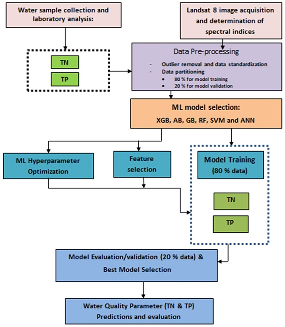
Figure 2. The overall study framework used in this study.

2.5.1 Adaboost regression

Adaboost regression (AB) is a typically boosting type ensemble ML algorithm introduced by Freund (2001). AdaBoost algorithm is a widely used iterative algorithm and a boosting algorithm with adaptive capabilities. It trains the weak learners and then integrates the trained weak learners to obtain a final model with enough strength level. After each iteration, the weights of the samples are adjusted, and the samples with more significant fitting errors will increase the corresponding weight values. The weak learner obtains a sequence of functions on the predicted values by iterative operations, and each prediction function is assigned a weight. The function with better prediction results has a larger corresponding weight, and, after several iterations, the final strong learner is obtained by weighing the weak learner function. The main idea is to integrate multiple weak learners to get the output of strong learners and make accurate predictions.

AB begins by fitting a regressor on the original dataset and then fits additional copies of the regressor on the same dataset but where the weights of instances are adjusted according to the error of the current prediction.

2.5.2 Random forest regression

Random forests are a nonparametric and tree-based ensemble technique proposed by Breiman et al. (2017). The random forest (RF) is a classification and regression system that uses many weak classifiers to classify and predict data. The developed classifiers are diverse and aggregated (Cutler et al., 2007). While continuing to select different training subsets, the RF selects the bagging method and produces associated decision trees at random. The RF algorithms use random attribute selection training techniques when picking the partition attribute of the node. With this quality, different data sets may be retrieved fast without repeating the process, which is preferable for data categorization. Finally, multiple decision trees are combined to form a random forest. Its final result is obtained by combining several weak classifiers by taking the mean. The error of the results depends on the classification ability of each tree and the correlation between them, which gives the results of the overall model have high accuracy and generalization performance. A decision tree used to solve regression problems is a regression tree divided by the minimal mean square deviation.

The predicted value of the dependent variable is obtained by averaging the predictions of all trees. The key to the algorithm is to determine the number of variables and the number of decision trees. The algorithm does not overfit as the number of trees increases, has good generalization performance, is more robust, and is suitable for dealing with high-dimensional, nonlinear complex problems.

2.5.3 Gradient boost regression

The Gradient boost regression (GB) is another popular machine learning algorithm that has the advantages of high accuracy, a fast training process, short prediction time, and a small memory footprint in various applications. GB gives a prediction model in the form of an ensemble of weak prediction models, which are typically decision trees. Like RF, the GB consists of an ensemble of decision trees, with a sequence of trees created, and each tree in the sequence focuses on the previous tree's prediction residuals. The innovation of the GB is its use of a nonparametric approach to estimating the basis function and using gradient descent to approximate the solution in function space. It is a powerful algorithm that can find any nonlinear relationship between the target variable and features. It has great usability and can deal with missing values, outliers, and high cardinality categorical values on data features (Friedman, 2002).

2.5.4 Support vector regression

Support vector regression (SVR) is a vector-based statistical learning technique that has proven good prediction. It is a regression variant of support vector machines. SVR is implemented using a kernel function, which is a nonlinear mapping function. The kernel function and a hyperplane linearly separate and transform the input data points into a high-dimensional space. As a result, the choice of kernel function significantly impacts model correctness. Commonly used kernel functions include linear, polynomial, Gaussian, sigmoid, spectral angle, and radial basis functions. An optimum solution can be found by iteratively adjusting hyperplanes based on the errors associated with them. The best way to choose the kernel function is to change the hyperplanes and reduce the errors associated with them iteratively (Mountrakis et al., 2011).

2.5.5 Extreme gradient boost regression

Extreme gradient boost regression (XGB), proposed by Chen and Guestrin (2016), is a scalable artificial intelligence algorithm for tree boosting. XGB is one of the implementations of this technique of GB which is one of the best-performing algorithms for supervised learning. XGB can be used to solve problems involving regression and classification. XGB improves prediction performance by reducing model bias and modifying the objective function of the GB algorithm. XGB is one of the implementations of GB, one of the best-performing algorithms for supervised learning. It can be used to solve problems involving regression and classification.

It is also an integrated learning method, a synthesis method that combines basis function and weight to form a good data-fitting effect. A gradient tree-based method that iteratively trains a series of weak learners (usually decision trees), each iteration attempting to correct the error of the previous iteration, and eventually combines these weak learners into a strong learner. Unlike traditional gradient-boosting decision trees, it adds regularization terms to the loss function and uses second-order Taylor expansion of the loss function as a fitting of the loss function, so it is more efficient when dealing with large data sets and complex models while preventing overfitting and improving generalization.

2.5.6 ANN

The ANN model is a type of nonlinear regression model that uses a set of feedforward neural networks to conduct an input-output mapping. It comprises three layers: an input layer, one or more hidden levels of computation nodes, and a computation node output layer. The highly linked framework of ANN models is recognized for transmitting information from the input layer through weighted connections and functional nodes known as transfer functions. These transfer functions make nonlinear data mapping to high-dimensional hyperplanes easier, allowing for the separation of data patterns and the formulation of a model output. ANN is fast and efficient used to handle a wide range of problems (Deo et al., 2017). We used one of the most common ANN structures utilized by many researchers is MLP architecture. MLP architecture has the advantage of being easy to use, and they can approximate any relationship between input and output through the typical three layers (Abiodun et al., 2018): the input layer, hidden layer and output layer. In this study, the most common transfer function called sigmoid transfer function, was used in the hidden layer, while a linear activation function was used at the input and output layers. In addition Adam optimization function and square error (MSE) loss were used.

2.6 Evaluation of model performance

This study evaluated the performances of ML algorithms by statistical metrics such as the determination coefficient (R²), Root Mean Square Error (RMSE) Nash-Sutcliff efficiency (NSE) and Mean Absolute Relative Error (MARE) (Niazkar et al., 2023).

$\begin{array}{ll}{R}^2=1-\frac{{\displaystyle {\sum }_{i=1}^n{\left(Y-y_i\right)}^2}}{\sqrt{{\displaystyle {\sum }_{i=1}^n{\left(y-y_i\right)}^2}}}& (1)\end{array}$

$\begin{array}{ll}RMSE=\sqrt{\frac{{\displaystyle {\sum }_{i=1}^n{\left(y_i-y\right)}^2}}{n}}& (2)\end{array}$

$\begin{array}{ll}MARE=\frac{1}{n}{\displaystyle \sum _{i=1}^n\left|\frac{y_i-y}{y_i}\right|}& (3)\end{array}$

$\begin{array}{ll}NSE=1-\frac{{\displaystyle {\sum }_{i=1}^n{\left(y_i-y\right)}^2}}{{\displaystyle {\sum }_{i=1}^n\left(y-\frac{{\displaystyle {\sum }_{i=1}^n{y}_i}}{n}\right)}}& (4)\end{array}$

where (Y, y_i, y, n) are mean true value, truth value, predicted value and number of data, respectively.

3 Results

3.1 Water quality of Lake Tana

Table 1 shows the water quality data used in the analysis. The maximum monthly average TN within the recording period was 2.95 mg/L in October 2016 at the end of rainy period, while the maximum monthly average observed TP was 1.75 mg/L observed in March 2021 during dry period. The seasonal variation of TN and TP are different. The data also showed that the TN concentration changes in Lake Tana between the minimum value of 0.1 mg/L during the dry period and the maximum value of 8.96 mg/L during the rainy period. For TP concentration, the range is between the minimum of 0.001 mg/L in December and 5.87 mg/L in October. Based on the TN and TP indicators, there is a potential risk of eutrophication incidence provided there is a coincidence of other relevant factors (temperature, chlorophyll, water transparency, oxygen level, etc.) (Yang et al., 2008; Li et al., 2015).

Table 1

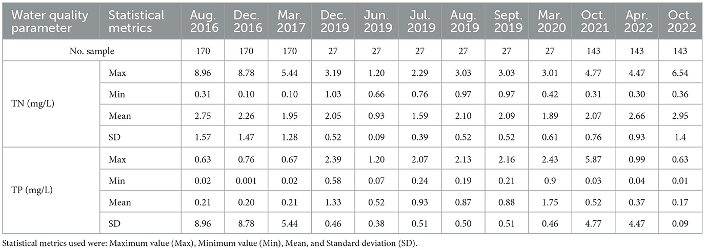
Table 1. Descriptive statistics of each water quality parameters for the month's data were collected.

3.2 Feature selection

Table 2 presents the best-selected features for each ML model for both considered water quality parameters. The analysis for the optimum number feature selection for TN and TP concentrations for other algorithms was shown in Supplementary Figures 1–10. It is evident from the result that the accuracy of most ML algorithms for both TN and TP concentrations increases from a minimum of five numbers of features to an optimum number of 10–13. A further increase in the number of features does not affect improving model accuracy except by significantly increasing calculation time. According to the results, the maximum number of features selected by AB and RF for TN concentration was 13. While SVR and XGB used 12 optimal features, GB used 10 features. The AB, RF, and SVR algorithms used 13 characteristics for TP concentration. GB and XGB, on the other hand, used only 12 of the best features. It is also worth noting that if a large number of features with comparable influence on a given dependent variable are provided to several ML models, it is less probable that all of the models will select the same features. As a result, the technique far outweighs prior approaches centered on offering a limited, smaller number of predetermined features.

Table 2

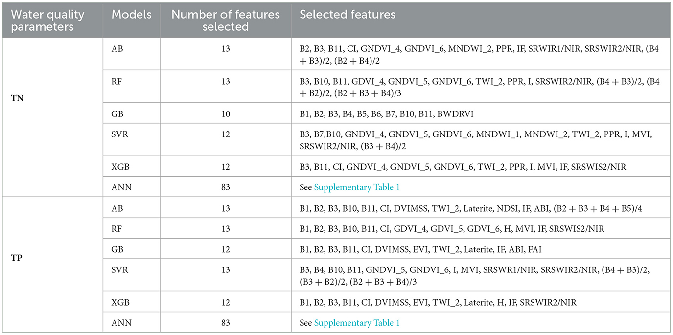
Table 2. Selected features for the different algorithms.

3.3 Evaluation of ML model's performance

Table 3 presents the results of the model performances analysis of the ML algorithms without binning technique applied to the dataset. The result indicated that ML algorithms have fairly good performances particularly of the ensemble algorithms. According to the result for TN retrieval modeling, the better performing models, XGB, GB, AB and RF algorithms had an R² of 0.69, 0.68, 0.67, 0.65 and NS index of 0.67, 0.69, 0.67, and 0.66, respectively. Similarly, for TP retrieval modeling, XGB, GB, AB and RF algorithms had an R² of 0.68, 0.67, 0.67, 0.68 and NS index of 0.66, 0.68, 0.69, 0.67, respectively. However, the study further tried to improve the performances of the ML algorithms to select the best-performing methods for TN and TP retrieval from RS imagery. In this study, the unsupervised data discretization method of equal width (Equal-W) binning in combination with Recursive Feature Elimination (REF) feature selection method were applied on the dataset. To search for an optimal bin number k for the discretization, we explored various bin sizes and chose the bin numbers of k = 10 for TN and k = 15 for TP as it consistently achieved good accuracies. The results of the performances of the ML algorithms after data binning technique was applied on the dataset are presented in Table 4. Also, Figure 3A shows the scatter plot between predicted and observed TN concentrations after data binning. The result indicated that the proposed ML algorithms caught the complex relationship between TN concentration and spectral indices of Landsat 8 OLI images with good performance of above 0.6 regression coefficients for most of the algorithms except ANN. However, XGB outscored all other algorithms with comparable performance metrics for TN concentration retrieval modeling with an R² of 0.80, NSE of 0.81, MARE of 0.043, and RMSE of 0.52 mg/L, while RF with an R² of 0.80, NSE of 0.79, MARE of 0.046, and RMSE of 0.52 mg/L took the second position with nearly the same values of performance metrics as XGB. AB and GB were found to perform next to XGB and RF. Comparing the performance of the ML models in terms of retrieval modeling of one parameter over the other, despite the fact that most models still performed well, the performance of ML algorithms for TN concentration was slightly superior than to that for TP concentration modeling (Table 4 and Figure 3B). The application of data binning significantly impacts the performance of ML algorithms. The technique could have been effective in reducing the impact of minor observation errors if models are not robust enough to tolerate over-fitting for a given dataset. In particular, for a small dataset, it may lower the chances of overfitting (Davaasambuu and Yu, 2015).

Table 3

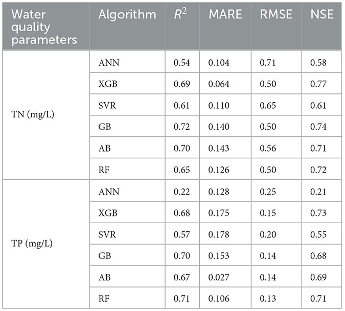
Table 3. The performance of six machine learning algorithms without binning applied on the dataset for predicting non-optical water quality parameters for both TN and TP using R², MARE, RMSE, and NSE.

Table 4

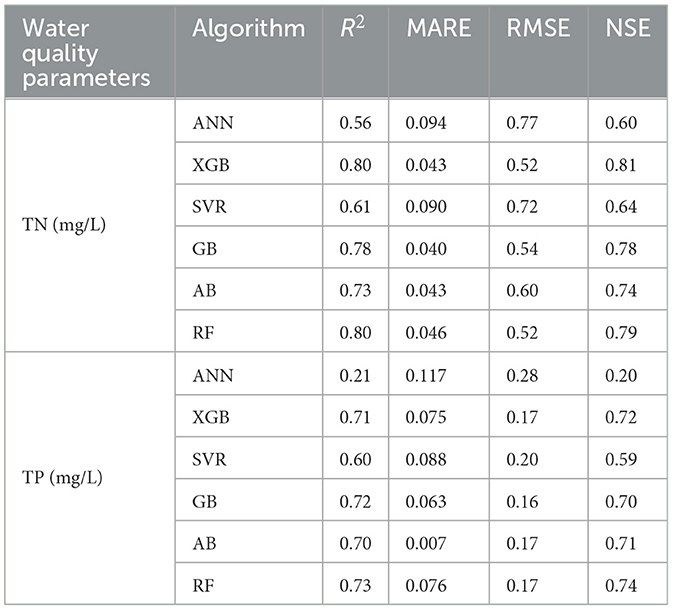
Table 4. The performance of six machine learning algorithms with binning applied on the dataset for predicting non-optical water quality parameters for both TN and TP using R², MARE, RMSE, and NSE.

Figure 3

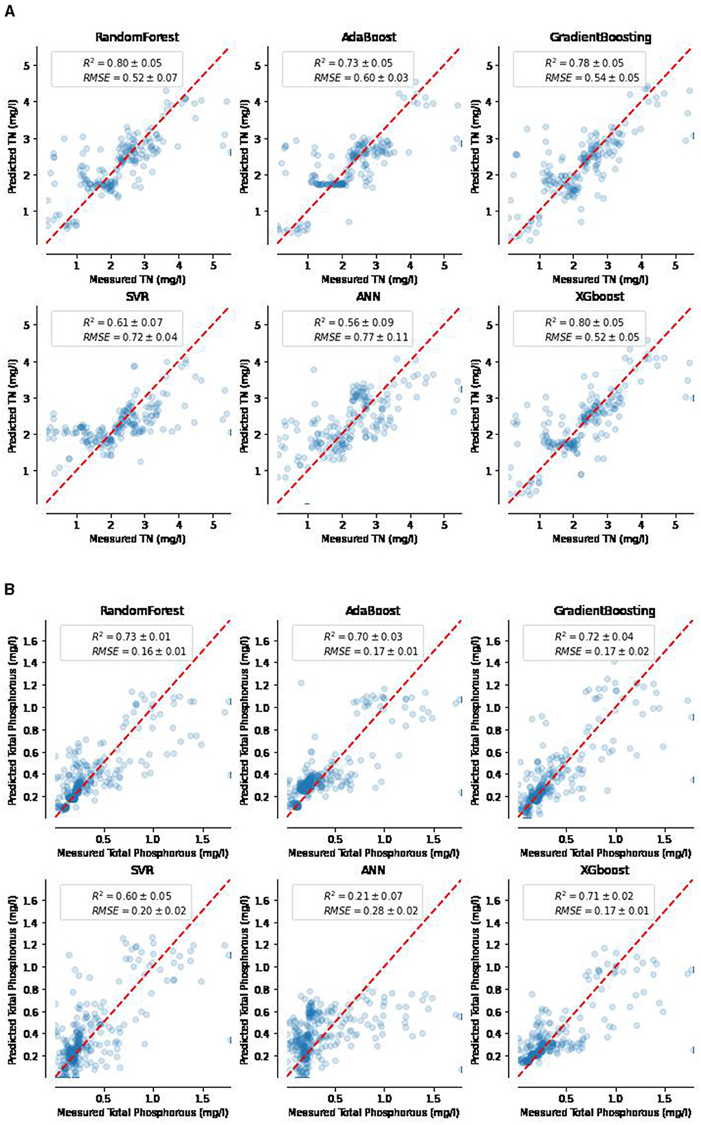
Figure 3. Scatter plot of observed vs. predicted Total Nitrogen (TN) mg/L using six different ML methods (A) and Total phosphorous (TP) in mg/L using six different ML methods (B).

Moreover, the correlation matrix results for the highest-performing algorithms were shown in Figure 4: XGB for TN concentration (left) and RF for TP concentration (right). The correlation matrix results for the other selected algorithms were presented in Supplementary Figures 11–20. Multiple band combinations were discovered to be the most important features in the retrieval of the two water quality parameters. Hence, two single-bands (B3 and B11) were found to be relevant features in determining TN using the XGB algorithm. In contrast, about five single-band features (B1, B2, B3, B10, and B11) were found to be important in features for building sound ML retrieval algorithm for TP concentration of the lake using RF algorithm. The XGB algorithm (Figure 4: left), show there were strong positive correlations between TN and B3, as well as SRSWIR2/NIR, with a correlation coefficient, r of around 0.45. Furthermore, TN had a substantial negative correlation with TWI_2, I, and IF, with r values around −0.42, respectively. TN also had a negative and substantial correlation with B3, CI, GNDVI_4, GNDVI_5, and GNDVI_6, with r ranging from −0.25 to −0.41. The best-performing algorithm for TP retrieval, the RF algorithm (Figure 4: right), the correlation between TP and B1, B2, and B3 was between −0.15 and −0.19. TP with B10, B11, and SRSWIR2/NIR had a positive correlation with r of 0.20, 0.26, and 0.4, respectively. There was a substantial negative association between TP and CI, GNDVI_4, GNDVI_5, GNDVI_6, and IF, with r-value ranging from −0.37 to −0.4. Overall ML models with selected features that highly positively or negatively correlated with the target variables (TN and TP concentrations) performed better. As a result, the correlation matrix result demonstrates that the selected features (Table 2) have the potential to be used to build a retrieval algorithms for TN and TP concentrations from Landsat 8 OLI images.

Figure 4

Figure 4. Correlation matrix of TN using XGB (A) and of TP using RF (B).

4 Discussion

4.1 Long-term temporal trend of TN, TP, and TN:TP ratio

To examine the model's effectiveness for long-term trend analysis, the yearly spatial average TN and TP concentrations from 2013 to 2021 were predicted using the best-performing algorithms, XGB and RF, respectively. The ratio of TN and TP was calculated using the derived TN and TP concentrations. The retrieved data were compared to TN, TP, and TN:TP ratio data published in the literatures. Wondie et al. (2007) in 2003 and 2004, Goshu and Aynalem (2017) in 2010, Ewnetu et al. (2014) in 2014, and Tibebe et al. (2019) in 2017 provided data on dissolved Nitrate. Dersseh et al. (2022) provided the TN and TP data, which was partly used in this study. Even though the retrieved average TN concentration over the lake varies less from year to year and is roughly equivalent to 0.8 mg/L (Figure 5), the same was observed in prior findings that Lake Tana's yearly spatial average TN concentration did not show a discernible trend from 2013 to 2021. Our predictions seem to underestimate the TN concentration when compared to Dersseh et al. (2022) (the green triangles) in which these data indicate specific values within particular months. The disparity could, therefore, be attributed to the use of yearly average reflectance data in this study unlike the monthly data in Dersseh et al. (2022).

Figure 5

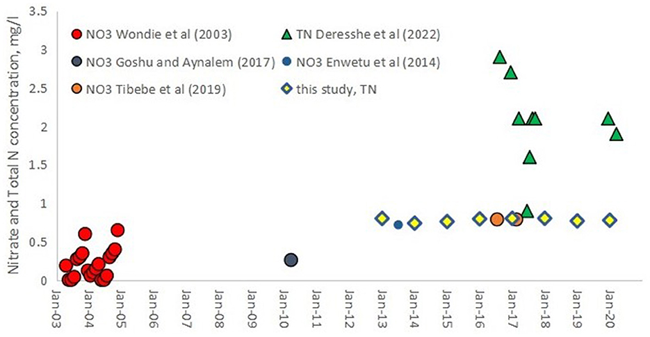
Figure 5. Available nitrate and total N concentrations in Lake Tana from 2003 to 2020 (Source: Dersseh et al., 2022) and TN trend in Lake Tana retrieved from Landsat OLI 8 using XGB from the year 2013–2020. The names in the legend refer to the first author of the publication in which the data are listed.

Unlike TN, the yearly spatial average of TP concentration in the lake has been increased since 2013, rising from 0.075 mg/L in 2013 to about 0.42 mg/L in 2021 (Figure 6). Similarly, the computed TN: TP ratios from this study were compared with those from Dersseh et al. (2022). As shown in Figure 7, the TN:TP trend followed an exponentially dropping trend from 10 in 2013 to a little < 2 in 2021, like the finding of Dersseh et al. (2022). Figure 8 informs that the lake is changing from the phosphorus limiting to nitrogen limiting based on the Redfield weight ratio (Redfield, 1958). This confirms that the coupled approach of ML with RS helps to assess the trend of non-optical water quality parameters in the absence of in-situ measurements.

Figure 6

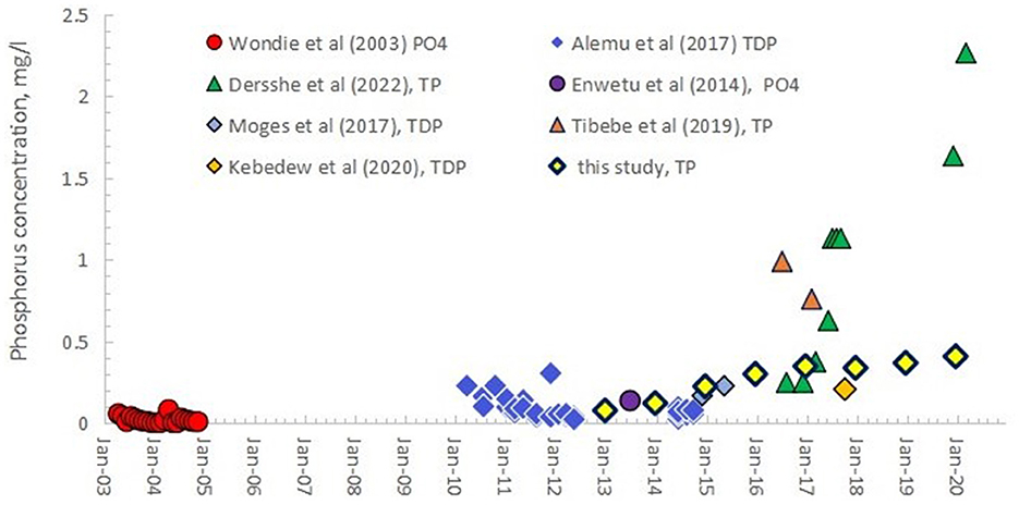
Figure 6. Published and observed concentrations of orthophosphate (PO4), soluble reactive phosphorus (SRP), total dissolved phosphorus (TDP) on filtered samples, and total phosphorus (TP) on unfiltered samples in lake Tana from 2003 to 2020 (Source: Dersseh et al., 2022) and TP trend in Lake Tana retrieved from Landsat OLI 8 using RF from the year 2013–2021. The names in the legend refer to the first author of the publication in which the data are listed.

Figure 7

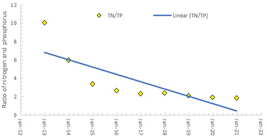
Figure 7. Calculated nitrogen phosphorus ratios on a weight basis in Lake Tana retrieved from Landsat 8 OLI image from 2013 to 2021.

Figure 8

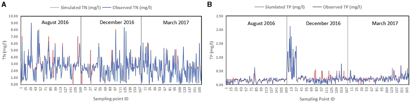
Figure 8. Observed vs. Predicted TN (A) and TP (B) in mg/l at the 170 sampling points (The sampling points are shown in Figure 1).

4.2 Spatial monthly TN and TP concentrations prediction

To assess the ability of the approach to capture the spatiotemporal patterns under different seasons, predictions were made for 3 months (August 2016, December 2016, and March 2017), during which in-situ observations were made in previous studies. The predictive power of the best-performing algorithms XGB for TN and RF for TN were presented in Figures 8A, B. The figure shows the observed vs. predicted TN and TP concentrations in mg/L at all sampling points shown in Figure 1. The plot showed a relatively a good match between the observed and the predicted water quality parameters, highlighting the effectiveness of ML models in predicting them. In addition, we did spatial-temporal map of observed and predicted TN and TP concentrations for August 2016, December 2016, and March 2017 in Figures 9, 10 using inverse distance weight approach.

Figure 9

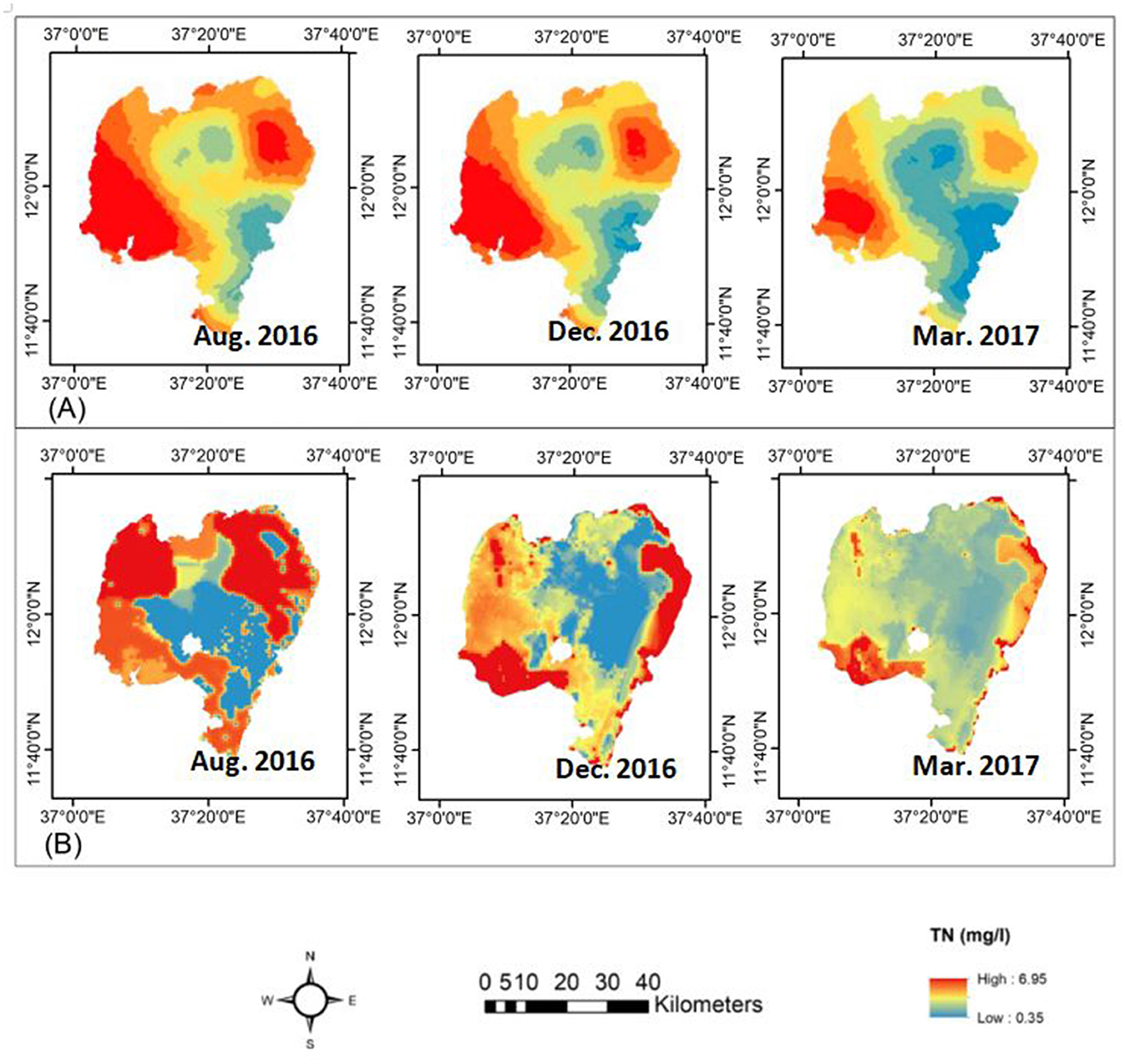
Figure 9. (A) Observed TN (mg/L) for August 2016, December 2016, and March 2017, and (B) Predicted TN for August 2016, December 2016, and March 2017 using the XGB algorithm.

Figure 10

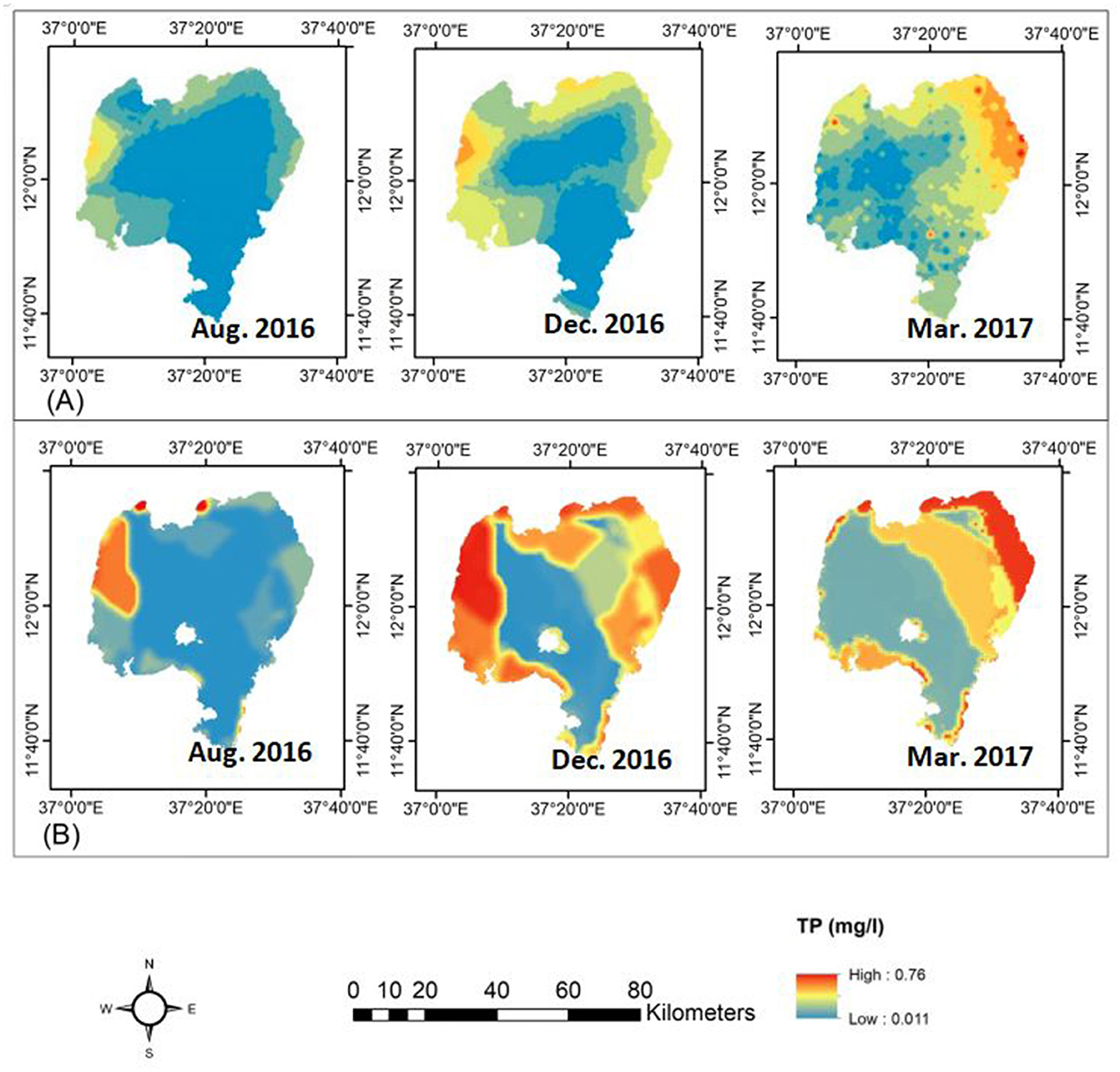
Figure 10. (A) Observed TP (mg/L) for August 2016, December 2016, and March 2017, and (B) Predicted TP for August 2016, December 2016, and March 2017 using the RF algorithm.

Figure 9B, shows the predicted TN concentrations variation over the lake using XGB algorithm for August 2016, December 2016, and March 2017. The spatial variations of TN concentrations showed a clear difference among the 3 months: higher in August, decreased in December, and lowest in March. Lake Tana water's lowest TN concentration level was predicted at 0.35 mg/L, higher than the observed minimum of 0.1 in December 2016 and March 2017 (Table 1). On the other hand, the maximum monthly predicted TN concentration was 6.95 mg/L in October which was lower than the 8.96 mg/L observed in August 2016 (Table 1). The result of this study showed the TN concentration of the lake has two distinct seasonal patterns, one in the southern part where Gilgel Abay River joins the lake, and one in the northeastern and eastern part, where Megech, Gumera and Rib Rivers join the lake. According to the spatial distributions of TN concentrations mapped by Dersseh et al. (2019) from observed data (Figure 9A), the western part and northeastern part of the lake had the highest concentration of TN in all the months with little or no difference from month to month while the predicted concentrations ranged from 0.51 to 5.8 mg/L. Our prediction showed similar results, though the minimum value seemed slightly overestimated compared to observations. Furthermore, the spatial seasonal pattern showed an agreement in all 3 months.

Similarly, the predicted TP concentrations using the RF algorithm for August 2016, December 2016, and March 2017 (Figure 10B) showed similar spatiotemporal patterns across the lake as shown in Figure 10A: the lake's southern, northeastern, and central regions of the lake. The spatial distribution of TP concentration revealed that TP concentration was lower in August and increased in December and March. On the other hand, the TP concentration in the lake's eastern section increased to the southeastern part in December before shifting to the northeastern part in March. For the most central or pelagic part, the TP concentration remained constant. Thus, the prediction of TP concentrations revealed that concentrations were higher in the western portion of the lake than in August, but they were higher in the northeastern section in March.

The lowest projected TP concentration level in Lake Tana water was 0.011 mg/L, which is higher than the measured level of 0.001 mg/L in December 2016. The maximum monthly average predicted TP concentration in March 2017 was 0.76 mg/L, which was slightly higher than the 0.67 mg/L recorded at the same time. Our findings closely matched the ranges and spatial distributions of TP concentrations (Figure 10A) found by Dersseh et al. (2019) and Kebedew et al. (2020). The spatiotemporal fluctuations in TN and TP concentrations could mainly relate to mixing by wind and lake depth (Kebedew et al., 2023).

4.3 Performance of ML Algorithms

The attempt to retrieve TN and TP concentrations from RS using six selected ML algorithms for Lake Tana water resources showed a reasonable accuracy with most of the ML algorithms particularly with the ensemble models. However, these water quality prediction models based on ML algorithms still have some issues arising from the lack of appropriate data representation and resolution for model training. And due to the “shallow” learning mechanism of these models, their ability to address input features and capture the long-term correlation of time series is very limited (Wang et al., 2021). Furthermore, the uncertainty of TN and TP concentration prediction in the rainy season could be affected by weather conditions, especially cloud cover. As such poor data quality affects mostly ANN and SVR models more than the ensemble ML types.

In general, the result indicated that boosting-based regressions were shown to have superior accuracy when compared to the performances of ANN and SVR for both water quality metrics, similar to the findings in Leggesse et al. (2023) and Gao et al. (2024). The out performances of the boosting-based algorithms RF, AB, GRB, and XGB was most likely owing to their ability to deal with intricate pathways and perform predictions without the need for regular huge datasets. ML-based solutions are determined by the nature and qualities of the data and the performance of the learning algorithms. If the data is unsuitable for learning, such as incompleteness or non-representativeness, inaccuracy, inconsistency, duplication, or insufficient amount for training, the machine learning models may become ineffective or generate incorrect results (Zhang Y. et al., 2022).

While ML algorithms do not explicitly consider physical processes, they often require large datasets to operate effectively (Noori et al., 2020). Our dataset, consisting of intermittent monthly data, could be categorized as low frequency compared to higher-frequency daily or hourly data. When compared to less frequent field sampling, the more frequent water quality monitoring allows for a more comprehensive understanding of water quality dynamics and extremes, potentially enhancing the accuracy of ML models (Chen et al., 2020).

Table 1 was gathered from 27 sampling points for certain months, and from 170 locations in others. This variability in data collection may not adequately represent yearly, seasonal, and monthly time scales, which are typically assumed to capture temporal variability at different sampling frequencies. We implemented a data binning technique to address potential issues related to data imbalance, ultimately enhancing the model's accuracy. This technique was employed to mitigate the impact of minor observation errors.

Future research should focusing on enhancing the accuracy of the ML algorithms, with a comprehensive in-situ data gathering and selection of other remote sensing products such as sentinel-2. As a result, current dynamics and future changes should be strategically captured in the in-situ data with less cost to improve spatial and temporal water quality dynamics of the lake of nutrients, which is strongly advised. In addition, the research should concentrate on the proper selection of ML algorithms with strong temporal predictive potential, such as LSTMs (Hochreiter and Schmidhuber, 1997). Because of their higher convergence speed and ability to capture long-term correlation of time series, such ML methods may even perform better. They are also more stable and accurate, providing ideas for future research on water quality prediction. Another alternative is a hybrid model, which has received a lot of interest from AI researchers. These models have the advantage of integrating various models via an effective combination. Data preparation, parameter selection and optimization are two commonly utilized methods (Bai et al., 2021) for integrating various ML models.

5 Conclusions

Based on remote sensing image from Landsat 8 OLI and the in-situ water quality data of Lake Tana, this study assessed six machine learning algorithms (AB, RF, GB, SVR, XGB, and ANN) for retrieval of two not-optically active water quality indicators, TN and TP concentrations. In conclusion, most algorithms performed reasonably well for TN prediction and only the ensemble type and SVR algorithms performed well for TP prediction. Despite some inconsistencies, the results show that the ML models seemed to capture the spatio-temporal variability of the TN and TP concentrations. This confirms that the data derived using ML from remote sensing can inform researchers and decision-makers about the status and behavior of the lakes.

This study also discovered the advantages of image enhancement. Most of the features selected by the feature selection method were derived from or enhanced indices from the primary bands (Band 1–Band 11) of the Landsat 8 imagery. These derived or enhanced indices exhibited a correlation with observed Total Nitrogen (TN) and Total Phosphorus (TP) concentrations, surpassing the predictive power of the primary bands alone.

Integrating in-situ data, remote sensing-based earth observation, and ML-based modeling data plays a pivotal role in deriving the most approximate and up-to-date baseline or prediction for Lake Tana water quality. This comprehensive approach combines real-time measurements from in-situ data with the wealth of information obtained through remote sensing technologies (especially with image enhancement) and ML modeling techniques. The ultimate goal is to provide a holistic and precise understanding of the Lake Tana's current state of water quality. Beyond this, it also fosters future active engagement with stakeholders to co-design demand-driven water quality services such as digital services for Lake Tana and beyond.

Data availability statement

The raw data supporting the conclusions of this article will be made available by the authors, without undue reservation.

Author contributions

ESL: Conceptualization, Data curation, Formal analysis, Funding acquisition, Investigation, Methodology, Resources, Validation, Writing – original draft, Writing – review & editing. FAZ: Conceptualization, Methodology, Supervision, Writing – review & editing. DS: Supervision, Writing – review & editing. TE: Supervision, Writing – review & editing. SAT: Conceptualization, Funding acquisition, Methodology, Supervision, Writing – review & editing.

Funding

The author(s) declare financial support was received for the research, authorship, and/or publication of this article. This research was funded by “the International Development Research Center (IDRC)” and “Swedish International Development Cooperation Agency (SIDA)” through Artificial Intelligence for Development – AI4D Africa scholarship (http://africa.ai4d.ai) program of African Center for Technology Studies to collect data after 2020 and support the ESL.

Acknowledgments

This research was made possible through initial support provided by the U.S. Agency for International Development under the Feed the Future Evaluation of the Relationship between Sustainably Intensified Production Systems and Farm Family Nutrition (SIPS-IN) project (AID-OAA-L-14-00006) with additional support from the Feed the Future Innovation Lab for Small Scale Irrigation (contract no. AID-OAA-A-13-0055) to collect data before 2020. This work was also supported by the CGIAR Initiative on West and Central African Food Systems Transformation, which is grateful for the support of CGIAR Trust Fund contributors (http://www.cgiar.org/funders). We would like to acknowledge the assistance of Minyechel Gitaw, Aron Ateka, Abiy Gebeyhu, and Work Abunu for their valuable help to collect the necessary data for this study.

Conflict of interest

The authors declare that the research was conducted without any commercial or financial relationships that could be construed as a potential conflict of interest.

The author(s) declared that they were an editorial board member of Frontiers, at the time of submission. This had no impact on the peer review process and the final decision.

Publisher's note

All claims expressed in this article are solely those of the authors and do not necessarily represent those of their affiliated organizations, or those of the publisher, the editors and the reviewers. Any product that may be evaluated in this article, or claim that may be made by its manufacturer, is not guaranteed or endorsed by the publisher.

Supplementary material

The Supplementary Material for this article can be found online at: https://www.frontiersin.org/articles/10.3389/frwa.2024.1432280/full#supplementary-material

References

Abera, A., Verhoest, N. E., Tilahun, S., Inyang, H., and Nyssen, J. (2021). Assessment of irrigation expansion and implications for water resources by using RS and GIS techniques in the Lake Tana Basin of Ethiopia. Environ. Monit. Assess. 193, 1–17. doi: 10.1007/s10661-020-08778-1

PubMed Abstract | Crossref Full Text | Google Scholar

Abiodun, O. I., Jantan, A., Omolara, A. E., Dada, K. V., Mohamed, N. A., Arshad, H., et al. (2018). State-of-the-art in artificial neural network applications: a survey. Heliyon 4:e00938. doi: 10.1016/j.heliyon.2018.e00938

PubMed Abstract | Crossref Full Text | Google Scholar

Bai, Y., Liu, M. D., Ding, L., and Ma, Y. J. (2021). Double-layer staged training echo-state networks for wind speed prediction using variational mode decomposition. Appl. Energy 301:117461. doi: 10.1016/j.apenergy.2021.117461

Crossref Full Text | Google Scholar

Breiman, L., Friedman, J. H., Olshen, R. A., and Stone, C. J. (2017). Classification and Regression Trees. London: Routledge. doi: 10.1201/9781315139470

Crossref Full Text | Google Scholar

Bunting, L., Leavitt, P. R., Hall, V., Gibson, C. E., and McGee, E. J. (2005). Nitrogen degradation of water quality in a phospho-rus-saturated catchment: the case of Lough Neagh, Northern Ireland. Verh. Internat. Verein Limnol. 29, 1005–1008. doi: 10.1080/03680770.2005.11902835

Crossref Full Text | Google Scholar

Bygate, M., and Ahmed, M. (2024). Monitoring water quality indicators over Matagorda Bay, Texas, using landsat-8. Remote Sens. 16:1120. doi: 10.3390/rs16071120

Crossref Full Text | Google Scholar

Cao, Z., Ma, R., Duan, H., Pahlevan, N., Melack, J., Shen, M., et al. (2020). A machine learning approach to estimate chlorophyll-a from Landsat-8 measurements in inland lakes. Remote Sens. Environ. 248:111974. doi: 10.1016/j.rse.2020.111974

Crossref Full Text | Google Scholar

Chen, K., Chen, H., Zhou, C., Huang., Y, Qi, X., and Shen, R. (2020) Comparative analysis of surface water quality prediction performance identification of key water parameters using different machine learning models based on big data. Water Res. 171:115454. doi: 10.1016/j.watres.2019.115454

PubMed Abstract | Crossref Full Text | Google Scholar

Chen, T., and Guestrin, C. (2016). “XGBoost: a scalable tree boosting system,” in KDD '16: Proceedings of the 22nd ACM SIGKDD International Conference on Knowledge Discovery and Data Mining (New York, NY: Association for Computing Machinery), 785–794. doi: 10.1145/2939672.2939785

Crossref Full Text | Google Scholar

Claverie, M., Ju, J., Masek, J. G., Dungan, J. L., Vermote, E. F., Roger, J.-C., et al. (2018). The Harmonized Landsat and Sentinel-2 surface reflectance data set. Remote Sens. Environ. 219, 145–161. doi: 10.1016/j.rse.2018.09.002

Crossref Full Text | Google Scholar

Cutler, D. R., Edwards, T. C., Beard, K. H., Cutler, A., Hess, K. T., Gibson, J. C., et al. (2007). Random forests for classification in ecology. Ecology 88, 2783–2792. doi: 10.1890/07-0539.1

PubMed Abstract | Crossref Full Text | Google Scholar

Davaasambuu, K. B., and Yu, T. S. (2015). Self-optimization of handover parameters for long-term evolution with dual wireless mobile relay nodes. Future Internet 7, 196–213. doi: 10.3390/fi7020196

Crossref Full Text | Google Scholar

Deo, R. K., Russell, M. B., Domke, G. M., Woodall, C. W., Falkowski, M. J., Cohen, W. B., et al. (2017). Using landsat time-series and LiDAR to inform aboveground forest biomass baselines in Northern Minnesota, USA. Can. J. Remote Sens. 43, 28–47. doi: 10.1080/07038992.2017.1259556

Crossref Full Text | Google Scholar

Dersseh, M. G., Kibret, A. A., Tilahun, S. A., Worqlul, A. W., Moges, M. A., et al. (2019). Potential of water hyacinth infestation on Lake Tana, Ethiopia: a prediction using a GIS-based multi-criteria technique. Water 11:1921. doi: 10.3390/w11091921

Crossref Full Text | Google Scholar

Dersseh, M. G., Steenhuis, T. S., Kiberet, A. A., Enyew, B. M., Kebedew, M. G., Zimale, F. A., et al. (2022). Water quality characteristics of a water hyacinth infected tropical highland lake: Lake Tana, Ethiopia. Front. Water 4:774710. doi: 10.3389/frwa.2022.774710

Crossref Full Text | Google Scholar

Ewnetu, D. A., Bitew, B. D., and Chercos, D. H. (2014). Determination of surface water quality status and identifying potential pollution sources of Lake Tana: particular emphasis on the Lake Boundary of Bahirdar City, Amhara Region, North West Ethiopia, 2013. J. Environ. Earth Sci. 4, 88–97. doi: 10.20372/nadre:1547201708.57

Crossref Full Text | Google Scholar

Freund, Y. J. H. (2001). Greedy function approximation: a gradient boosting machine. Ann. Stat. 29, 1189–1232. doi: 10.1214/aos/1013203450

PubMed Abstract | Crossref Full Text | Google Scholar

Friedman, J. H. (2002). Stochastic gradient boosting. Comput. Stat. Data Anal. 38, 367–378. doi: 10.1016/S0167-9473(01)00065-2

Crossref Full Text | Google Scholar

Gao, L., Shangguan, Y. Z., Shen, Q., and Shi, Z. (2024). Estimation of non-optically active water quality parameters in zhejiang province based on machine learning. Remote Sens. 16:514. doi: 10.3390/rs16030514

Crossref Full Text | Google Scholar

Goshu, G., and Aynalem, S. (2017). “Problem overview of the lake Tana basin,” in Social and Ecological System Dynamics. AESS Interdisciplinary Environmental Studies and Sciences Series, eds. K. Stave, G. Goshu, and S. Aynalem (Cham: Springer), 9–23. doi: 10.1007/978-3-319-45755-0_2

Crossref Full Text | Google Scholar

Guo, H., Huang, J. J., Chen, B., Guo, X., and Singh, V. P. (2020). A machine learning-based strategy for estimating non-optically active water quality parameters using Sentinel-2 imagery. Int. J. Remote Sens. 42, 1841–1866. doi: 10.1080/01431161.2020.1846222

Crossref Full Text | Google Scholar

Hastie, A., Lauerwald, R., Ciais, P., Papa, F., and Regnier, P. (2021). Historical and future contributions of inland waters to the Congo basin carbon balance. Earth Syst Dyn 12, 37–62. doi: 10.5194/esd-12-37-2021

Crossref Full Text | Google Scholar

Hochreiter, S., and Schmidhuber, J. (1997). Long short-term memory. Neural Comput. 9, 1735–1780. doi: 10.1162/neco.1997.9.8.1735

PubMed Abstract | Crossref Full Text | Google Scholar

Kebedew, M. G., Kibret, A. A., Tilahun, S. A., Belete, M. A., Zimale, F. A., Steenhuis, T. S., et al. (2020). The relationship of lake mor-phometry and phosphorus dynamics of a tropical highland lake: lake Tana, Ethiopia. Water 12:2243. doi: 10.3390/w12082243

Crossref Full Text | Google Scholar

Kebedew, M. G., Tilahun, S. A., Zimale, F. A., Belete, M. A., Wosenie, M. D., Steenhuis, T. S., et al. (2023). Relating lake circulation patterns to sediment, nutrient, and water hyacinth distribution in a shallow tropical highland lake. Hydrology 10:181. doi: 10.3390/hydrology10090181

Crossref Full Text | Google Scholar

Kim, Y. H., Im, J., Ha, H. K., Choi, J. K., and Ha, S. (2014). Machine learning approaches to coastal water quality monitoring using GOCI satellite data. Gisci. Remote Sens. 51, 158–174. doi: 10.1080/15481603.2014.900983

Crossref Full Text | Google Scholar

Lan, L., Mingjian, G., Cailan, G., Yong, H., Xinhui, W., Zhe, Y., et al. (2023). An advanced remote sensing retrieval method for urban non-optically active water quality parameters: an example from Shanghai. Sci. Total Environ. 880, 0048–9697. doi: 10.1016/j.scitotenv.2023.163389

PubMed Abstract | Crossref Full Text | Google Scholar

Laraque, A., N'kaya, G. D. M., Orange, D., Tshimanga, R., Tshitenge, J. M., Mahé, G., et al. (2020). Recent budget of hydroclimatology and hydrosedimentology of the congo river in central Africa. Water 12:2613. doi: 10.3390/w12092613

Crossref Full Text | Google Scholar

Leggesse, E. S., Zimale, F. A., Sultan, D., Enku, T., Srinivasan, R., and Tilahun, S.A. (2023). Predicting optical water quality indi-cators from remote sensing using machine learning algorithms in tropical highlands of Ethiopia. Hydrology 10:110. doi: 10.3390/hydrology10050110

Crossref Full Text | Google Scholar

Li, X., Huang, T. L., Ma, W. X., Sun, X., and Zhang, H. H. (2015). Effects of rainfall patterns on water quality in a stratified reservoir subject to eutrophication: implications for management. Sci. Total Environ. 521–522, 27–36. doi: 10.1016/j.scitotenv.2015.03.062

PubMed Abstract | Crossref Full Text | Google Scholar

Liang, Q., Zhang, Y., Ma, R., Loiselle, S., and Hu, M. (2017). A MODIS-based novel method to distinguish surface cyanobacterial scums and aquatic macrophytes in Lake Taihu. Remote Sens. 9:133. doi: 10.3390/rs9020133

Crossref Full Text | Google Scholar

Mountrakis, G., Im, J., and Ogole, C. (2011). Support vector machines in remote sensing: a review. ISPRS J. Photogramm. Remote Sens. 66, 247–259. doi: 10.1016/j.isprsjprs.2010.11.001

Crossref Full Text | Google Scholar

Niazkar, M., Goodarzi, M. R., and Fatehifar, A. (2023). Machine learning-based downscaling: application of multi-gene genetic programming for downscaling daily temperature at Dogonbaden, Iran, under CMIP6 scenarios. Theor. Appl. Climatol. 151, 153–168. doi: 10.1007/s00704-022-04274-3

Crossref Full Text | Google Scholar

Noori, N., Kalin, L., and Isik, S. (2020). Water quality prediction using SWAT-ANN coupled approach. J. Hydrol. 590:125220. doi: 10.1016/j.jhydrol.2020.125220

Crossref Full Text | Google Scholar

Redfield, A. C. (1958). The biological control of chemical factors in the environment. Am. Sci. 46, 230A−221.

Google Scholar

Sagan, V., Peterson, K. T., Maimaitijiang, M., Sidike, P., Sloan, J., Greeling, B. A., et al. (2020). Monitoring inland water quality using remote sensing: potential and limitations of spectral indices, bio-optical simulations, machine learning, and cloud computing. Earth-Sci. Rev. 205:103187. doi: 10.1016/j.earscirev.2020.103187

Crossref Full Text | Google Scholar

Sagi, O., and Rokach, L. (2018). Ensemble learning: a survey. WIREs Data Min. Knowl. Discov. 8:e1249. doi: 10.1002/widm.1249

Crossref Full Text | Google Scholar

Schindler, D. W. (2012). The dilemma of controlling cultural eutrophication of lakes. Proc. R Soc. B 279, 4322–4333. doi: 10.1098/rspb.2012.1032

PubMed Abstract | Crossref Full Text | Google Scholar

Sishu, F. K., Tilahun, S. A., Schmitter, P., Assefa, G., and Steenhuis, T. S. (2022). Pesticide contamination of surface and groundwater in an ethiopian highlands' watershed. Water 14:3446. doi: 10.3390/w14213446

Crossref Full Text | Google Scholar

Sterner, R. W. (2008). On the phosphorus limitation paradigm for lakes. Internat Rev. Hydrobiol. 93, 433–445. doi: 10.1002/iroh.200811068

Crossref Full Text | Google Scholar

Taye, M. T., Haile, A. T., Fekadu, A. G., and Nakawuka, P. (2021). Effect of irrigation water withdrawal on the hydrology of the Lake Tana sub-basin. J. Hydrol. Reg. Stud. 38:100961. doi: 10.1016/j.ejrh.2021.100961

Crossref Full Text | Google Scholar

Tesfaye, A. (2024). Remote sensing-based water quality parameters retrieval methods: a review. East Afr. J. Environ. Nat. Resour. 7, 80–97. doi: 10.37284/eajenr.7.1.1753

Crossref Full Text | Google Scholar

Tibebe, D., Kassa, Y., Melaku, A., and Lakew, S. (2019). Investigation of spatiotemporal variations of selected water quality parameters and trophic status of Lake Tana for sustainable management, Ethiopia. Microchem. J. 148, 374–384. doi: 10.1016/j.microc.2019.04.085

Crossref Full Text | Google Scholar

Vijverberg, J., Sibbing, F. A., and Dejen, E. (2009). “Lake Tana: source of the Blue Nile,” in The Nile, ed. H. J. Dumont (Dordrecht: Springer), 163–192. doi: 10.1007/978-1-4020-9726-3_9

Crossref Full Text | Google Scholar

Wang, X., Wang, Y., Yuan, P., Wang, L., and Cheng, D. (2021). An adaptive daily runoff forecast model using VMD-LSTM-PSO hybrid approach. Hydrol. Sci. J. 66, 1488–1502. doi: 10.1080/02626667.2021.1937631

PubMed Abstract | Crossref Full Text | Google Scholar

Wieczorek, J., and Guerin, C. (2022). K-fold cross-validation for complex sample surveys. Stat 11:e454. doi: 10.1002/sta4.454

Crossref Full Text | Google Scholar

Wondie, A., and Mengistou, S. (2014). Seasonal variability of secondary production of cladocerans and rotifers, and their trophic role in Lake Tana, Ethiopia, a large, turbid, tropical highland lake. Afr. J. Aquat. Sci. 39, 403–416. doi: 10.2989/16085914.2014.978835

PubMed Abstract | Crossref Full Text | Google Scholar

Wondie, A., Mengistu, S., Vijeverberg, J., and Dejen, E. (2007). Seasonal variation in primary production of a large high altitude tropical lake (Lake Tana, Ethiopia): effects of nutrient availability and water transparency. Aquat. Ecol. 41, 195–207. doi: 10.1007/s10452-007-9080-8

Crossref Full Text | Google Scholar

Yang, X. E., Wu, X., Hao, H. L., and He, Z. L. (2008). Mechanisms and assessment of water eutrophication. J. Zhejiang Univ. Sci. B. 9, 197–209. doi: 10.1631/jzus.B0710626

PubMed Abstract | Crossref Full Text | Google Scholar

Zhang, H., Xue, B., Wang, G., Zhang, X., and Zhang, Q. (2022). Deep learning-based water quality retrieval in an impounded Lake using landsat 8 imagery: an application in Dongping Lake. Remote Sens. 14:4505. doi: 10.3390/rs14184505

Crossref Full Text | Google Scholar

Zhang, L., Zhang, L., Cen, Y., Wang, S., Zhang, Y., Huang, Y., et al. (2022). Prediction of total phosphorus concentration in macrophytic lakes using chlorophyll-sensitive bands: a case study of Lake Baiyangdian. Remote Sens. 14:3077. doi: 10.3390/rs14133077

Crossref Full Text | Google Scholar

Zhang, Y., Jin, S., Wang, N., Zhao, J., Guo, H., Pellikka, P., et al. (2022). Total phosphorus and nitrogen dynamics and influencing factors in dongting lake using Landsat Data. Remote Sens. 14:5648. doi: 10.3390/rs14225648

Crossref Full Text | Google Scholar