Using index and physically-based models to evaluate the intrinsic groundwater vulnerability to non-point source pollutants in an agricultural area in Sardinia (Italy)

This research aims at studying the intrinsic vulnerability of groundwater to diffuse environmental pollutants in the Muravera coastal agricultural area of Sardinia, Italy. The area faces contamination risks arising from agricultural practices, especially the use of fertilizers, pesticides, and various chemicals that can seep into the groundwater. The study examined the interplay among hydrological elements, including soil characteristics, groundwater depth, climate conditions, land use, and aquifer properties. To do that, the outcomes of FLOWS 1D physically-based agrohydrological model were analyzed in parallel with those of the overlay-and-index model SINTACS, in a sort of reciprocal benchmarking. By using FLOWS, water movement and solute transport in the unsaturated zone were simulated by, respectively, solving the Richard Equation (RE) and the Advection-Dispersion equation (ADE). As such, this model allowed to account for the role of soil hydraulic and hydro-dispersive properties variability in determining the travel times of a conservative solute through the soil profile to the groundwater. For FLOWS simulations, a complete dataset was used as input, including soil horizons, soil physical and hydraulic properties of 36 soil profiles, average annual depth to groundwater table at each soil profile (ranging from 1 to 50 meters), and climatic temporal series data on rainfall and evapotranspiration. Detailed analyses of travel times for the movement of 25, 50, 75, and 100% of the solute mass to reach groundwater were conducted, revealing that the depth to groundwater predominantly influences vulnerability. This result was coherent with SINTACS vulnerability map due to the large impact of the depth to groundwater on SINTACS analysis.

1 Introduction

The pollution of natural water bodies represents a serious environmental problem of global worth. Commonly considered to be limited to specific point sources like waste disposal sites, industrial spills, mine activities, there is now full evidence that modern agriculture can also lead to what is termed non-point source (NPS) pollution, i.e., a diffuse pollution across large areas (McCoy et al., 2015). Agrochemicals (fertilizers, pesticides…) are nowadays recognized to be the main responsible for the NPS pollution waters (United Nations Environment Programme/Mediterranean Action Plan and Plan Bleu, 2020). Actually, NPS pollution is frequent in areas of intensive agriculture and livestock activity (Kanter and Brownlie, 2019). In these areas, in Europe for example, nitrate concentrations frequently exceed the limit of 50 mg NO₃/L for drinking water (Lawniczak et al., 2016; Biddau et al., 2019). Compared to point-sources pollution, which is generally limited in areal extent (thousand square meters), time extent (hours or days), highly concentrated, even orders of magnitude higher than regulatory limits, NPS pollution is much more subtle in the short period, as it typically occurs continuously over long time periods across a whole groundwater basin (Xepapadeas, 2011).

The repercussions of such contamination extend beyond just the degradation of soil and water quality, posing tangible risks to both human health and ecosystem integrity (Kanter et al., 2020). Addressing NPS pollution requires comprehensive and collaborative efforts involving various stakeholders, including government agencies, industries, farmers, and communities. In the perspective of reducing pollution of water bodies, a set of rules and regulatory mechanisms have been set out in national and supranational regulations aiming at the improvement and preservation of the water bodies quality. In Europe, the Nitrates Directive (91/676/CEE), the Water Framework Directive (WFD, 2000/60/EC) and, more recently, the new Green Deal strategy, including a so-called Zero Pollution Plan, have all prompted the need to develop methodologies and tools for evaluating the quality of natural water bodies and predicting their vulnerability to pollution. As an example, the Nitrate Directive imposed the identification of Nitrate Vulnerable Zones (NVZ), where farmers are required to comply with specific limits of inorganic fertilizers and organic slurry application rates (not more than 170 Kg of N/ha/yr).

To know the susceptibility of an aquifer to contamination from the surface, vulnerability must be defined; hereafter, with the term vulnerability we will refer to the probability of percolation and diffusion of contaminants from the ground surface into the groundwater system. There are two main ways to assess aquifer vulnerability: intrinsic vulnerability and specific vulnerability (Vrba and Zaporozec, 1994; Moraru and Hannigan, 2018). Intrinsic vulnerability considers the natural characteristics of the aquifer system itself, such as the geology, hydrology, and soil properties. These factors influence how quickly and easily contaminants can move through the vadose zone and reach the groundwater. Specific vulnerability considers the chemiodynamic properties of the specific contaminant or pollutants of concern (toxicity, persistence, decay, interactions with the aquifer and soil solid particles).

Predictive tools are now available for understanding and predicting NPS pollution coming from agrochemicals use, in terms of impact on soils, as well as on surface and subsurface water (Yuan et al., 2020). Different modelling solutions exist, mainly differing on the role of the vadose zone and its horizontal and vertical variability in the predictive models (Bordbar et al., 2024). Different approaches based on spatial attributes such as soil type, topography, average depth to water table, prevailing cropping practices, as well as use of fertilizers and pesticides have been employed to obtain a spatial understanding of contaminant transport potential. According to Corwin et al. (1997), these categories of models, coupled to Geographical Information Systems (GIS), have been generally used for screening purposes. These approaches range from: (1) Regression models, based on statistical associations (frequently multiple regression) between the spatial attributes described above and the occurrence of groundwater pollution (e.g., Nolan et al., 1997, 2002); (2) Overlay and index models, based on the calculation of an index of NPS pollutant mobility based on simple models describing steady-state solute transport. The latter may be classified as: (i) process-based index if somehow accounting for transport processes (e.g., Rao’s attenuation factor model) (Jury et al., 1983; Rao et al., 1985); (ii) property-based index models, if accounting for hydrogeologic setting [e.g., DRASTIC (Aller and Thornhill, 1987) or SINTACS (Civita and De Maio, 1997, 2004)]. SINTACS is recognized as one of the most extensively utilized rating-based approaches in Mediterranean environments (Civita and De Maio, 2004; Jahromi et al., 2021); and (iii) hybrid methods that integrate different approaches, such as ISIS method (Gogu and Dassargues, 2000).

The primary advantage of overlay-and-index models lies in the availability of certain factors, such as rainfall and depth to groundwater across large areas, making them suitable for regional-scale assessments. These models are utilized to estimate groundwater variability when there is no adequate information on soil variability, by assuming that the soil units are macroscopically uniform, thus allowing to statically identify macro-areas with relatively larger or lower vulnerability. On the other hand, their principal weakness lies in the quite subjective assignment of numerical values to descriptive entities and the relative weights assigned to different attributes (Masroor et al., 2021; Jain, 2023). Also, while these approaches may offer adequate average depictions of contaminant vulnerability across large areas, they lack consideration for significant contaminant transport mechanisms and do not provide time evolution of contaminant fluxes to groundwater (Severino et al., 2010). This way, there are no possibilities to gain insights into the time evolution of contaminant fluxes to groundwater nor on the contaminant transport mechanisms, which may be indispensable for specific vulnerability attenuation, for example by changing soil management. Moreover, while this approach may be appropriate for certain genetic soils consisting of intrinsic genetic horizons and do not vary significantly in the thickness of every horizon within a certain area, it falls short for alluvial soils. Alluvial soils exhibit highly intricate textural layering, with significant variation in thickness between horizons. Unlike genetic soils, the impact of textural layering on regional water flow and solute transport in alluvial soils may be quite critical due to sometimes abrupt transitions between different textural layers within the soil profile.

In contrast, hydrodynamic process-based models, describing transport processes in the vadose zone (the region from the soil surface to the groundwater table) provide a more comprehensive understanding of contaminant transport processes (refer to Stewart and Loague, 2003; Troldborg et al., 2008, among others). Generally, they are transient-state transport models able to describe some or all the process involved in solute transport in the vadose zone: water flow, solute transport, chemical reactions (adsorption–desorption, exchange, dissolution, precipitation, etc.) root growth, plant water uptake, vapor phase flow, degradation, and dispersion/diffusion (Corwin et al., 1997). Also, a primary advantage of employing a process-based approach lies in its capability to conduct scenario analyses under dynamically changing temporal and spatial conditions, such as changes in climatic patterns. This is why they are becoming common tools for evaluating vulnerability and its spatial distribution (see Stewart and Loague, 2003; Troldborg et al., 2008, among others). Nevertheless, even when these models are used in 1D configurations, their use still involves complex parameterizations and knowledge of soil profiles spatial variability, which can limit their use in large scale applications. As an example, these models need detailed information on both the vertical and horizontal spatial variability of hydraulic properties, as well as hydrodispersive properties, which are frequently lacking. In many cases, the problem has been partly overcome by applying indirect estimations techniques for hydraulic properties such as pedo-transfer functions (PTFs) (Wösten et al., 2001; Vereecken et al., 2010; Hassan et al., 2022), even at the cost of some additional uncertainty (Wang et al., 2009). Furthermore, compared to the index models, these unsaturated-zone hydrological models do not account for the groundwater spreading velocity.

In any case, when the spatial information on soil variability is available, these models provide a powerful tool for identifying contaminant transport mechanisms, assessing the importance of within soil class variability of transport parameters, analyzing the role of soil management and, overall, estimating temporal contaminant behavior and transport through the whole soil profile and to groundwater.

However, in a prudential approach to the issue, one should be aware that the concept of vulnerability always keeps some ambiguities, as it may only provide a relative indication of where contamination is most likely to occur and how the contamination develops in space and time into the groundwater. As an example, while on one side the unsaturated-zone hydrological models may provide a detailed description of the travel times to the groundwater, compared to the index models, they do not account for the contaminant spreading velocity into the aquifer, which represent their main weakness.

In this sense, we maintain that the most reasonable approach for gaining confidence in vulnerability mapping is by using diverse modelling approaches in a complementary way. For example, overlay and index models may provide a macroscopic vulnerability mapping, by identifying macro-areas of vulnerability based on macroscopic descriptions of the physical system, including the role of aquifer characteristics. These results may be completed by outputs of physically based transient state hydrodynamic models, which may allow identifying the role of hydrological variability within soil units (generally dealt with as homogeneous in macroscopic vulnerability approaches) on the travel time of pollutants through the soil profile and to groundwater, as well as identifying actual different transport mechanisms depending on the variability of hydro-pedological characteristics in the investigated areas. This is exactly the approach used in this paper, whose primary aim is to analyze and compare the outcomes of two vulnerability assessment methods, one based on the use of the known SINTACS model (Civita and De Maio, 1997), for identification of macroscopic vulnerability areas, and the other using a physically-based agrohydrological model, known as FLOWS (Coppola et al., 2015a,b, 2019; Hassan et al., 2023), allowing to gain more insights in the role of the hydrological behavior of the unsaturated zone in determining the variability of travel times within the SINTACS. In doing that, due to their different conceptual approaches, the combination of the two models allows obtaining a twofold objective: (1) Firstly, the two models complement each other; the SINTACS model accounts for the characteristics of the aquifer, which are not considered in FLOWS; and (2) the outcomes of the two models may be used for a reciprocal benchmarking when applied to the same case study. The latter is an extremely relevant issue, given the general lack of groundwater pollution measurements, to be used for the validation of alternative vulnerability models. In such a context, a “cross-validation” of different models may be the only viable approach, by also considering that, even in the case of available concentration measurement, these may not necessarily be correlated with solute travel times through the unsaturated zone to the groundwater in the case of highly transmissive aquifers.

In this direction, in this paper the SINTACS and FLOWS models were both applied to predict the groundwater vulnerability in the Muravera Plain, in the south-east of Sardinia Island – Italy. A similar approach was recently used in Marchfeld Region in Austria (Fusco et al., 2024). The strength of the analysis presented in our study lies in the fact that a large dataset is available in terms of hydrological regime, hydrogeological settings, variability of soils and related properties. The two approaches were both used to identify a so-called intrinsic vulnerability, that is a vulnerability related only to the intrinsic physical characteristics of the system, with no consideration to the chemiodynamic properties of specific pollutants. As such, in FLOWS the travel times of a conservative element (i.e., Cl⁻) were simulated, with the real top (rainfall, evaporation, …) and bottom (depth to water table) boundary conditions taken from the available dataset.

2 Materials and methods

2.1 The models

2.1.1 SINTACS model

SINTACS operates as a parametric system utilizing scores and weights to delineate regions within a specified area exhibiting diverse levels of susceptibility to pollution. This is accomplished through the assessment of seven critical factors: (1) depth to water table, (2) effective infiltration, (3) condition of the unsaturated zone, (4) type of land cover, (5) characteristics and (6) hydraulic conductivity of the aquifer, and (7) slope.

The evaluation process entails assigning a Pi score ranging from 1 to 10 to each of the seven parameters based on the SINTACS chart combinations. Additionally, to emphasize the varying significance of parameters in specific hydrogeological contexts and considering the effects of human influence and land-use practices, a weight (W_i coefficient) ranging from 1 to 5 is allocated to each parameter proposed by Civita and De Maio (2004) who indicate five different strings of weights to be assigned depending on the site-specific hydrogeological and impact situations (Table 4 in Civita and De Maio, 2004). Subsequently, the SINTACS index is derived, with values ranging from 26 to 260. This range is segmented into six classes to generate the final intrinsic vulnerability map of the examined aquifer. The intrinsic vulnerability index (I) is categorized into six classes as follows:

1. I > 210 very high vulnerability.

2. 186 < I ≤ 210 high vulnerability.

3. 140 < I ≤ 186 moderately high vulnerability.

4. 105 < I ≤ 140 medium vulnerability.

5. 80 < I ≤ 105 low vulnerability.

6. I ≤ 80 very low vulnerability.

2.1.2 FLOWS model

FLOWS (FLOw of Water and Solutes in agri-environmental systems) is a dynamic predictive model of water flow and solute transport processes (nutrients, salts, contaminants,…) in agri-environmental systems (Coppola et al., 2009, 2014, 2015a,b), which allows, among other things, a physically based prediction of the deep percolation flows (beyond the area explored by the root systems) of water and solutes, also allowing the estimation of groundwater recharge and transfer of any pollutants to the groundwater (e.g., nitrates, pesticides, heavy metals). The numerical code is written in MATLAB and is based on a standard finite difference solution scheme of the differential equations that govern the motion of water and the transport of solutes in partially saturated porous media (Coppola and Randazzo, 2006).

The model simulates the water flow by solving the Richards equation and the transport of solutes (tracers, adsorbed, volatile and reactive solutes) by solving the convection–dispersion equation and therefore allows to deal with general environmental problems related to water flow and the transport of contaminants with a rigorous physically based approach. For agricultural management purposes, FLOWS allows the integrated simulation of chemical transformations and the transport of organic and inorganic carbon, nitrogen and phosphorus simultaneously with the simulation of water contents and related flows. It also allows irrigation management, optimizing irrigation times and volumes according to a criterion based on the average water potential in the root zone. FLOWS also simulates water and nutrient flows towards artificial drainage and surface runoff. Furthermore, the model offers the possibility to run multi-site simulations, which can be particularly important for spatially distributed simulations, as well as for simulations carried out in a stochastic environment (e.g., Monte Carlo).

2.1.2.1 Soil water flow and solute transport with FLOWS

FLOWS simulates vertical transient water flow by numerically solving the 1D form of the Richards equation (Eq. 2) using an implicit, backward, finite differences scheme with explicit linearization:

$\begin{array}{ll}C\left(h\right)\frac{\partial h}{\partial t}=\frac{\partial }{\partial z}\left(K\left(h\right)\frac{\partial h}{\partial z}+K\left(h\right)\right)-S_w& (1)\end{array}$

where $C\left(h\right)$ = dθ/dh [L⁻¹] is the soil water capacity, θ is the water content (dimensionless), $h$ [L] is the soil water pressure head, $t$ [T] is time, $z$ [L] is the vertical coordinate being positive upward, $K\left(h\right)$ [L T⁻¹] is the hydraulic conductivity and $S_w\left(h\right)$ [T⁻¹] is a sink term describing water uptake by plant roots. Several water retention and hydraulic conductivity models can be selected. In this study, we assumed that the soil hydraulic properties can be described by the unimodal van Genuchten-Mualem model (Mualem, 1976; van Genuchten, 1980):

$\begin{array}{cc}\hfill {\mathrm{S}}_{\mathrm{e}}=\frac{\theta -{\theta }_{\mathrm{r}}}{{\theta }_{\mathrm{s}}-{\theta }_{\mathrm{r}}}={\left[1+{\left|{\alpha }_{\mathrm{V}\mathrm{G}}\mathrm{h}\right|}^{\mathrm{n}}\right]}^{-\mathrm{m}}\hfill & \hfill \mathrm{h}<0\hfill \\ \hfill \theta ={\theta }_{\mathrm{s}}\hfill & \hfill \mathrm{h}\ge 0\hfill \end{array}\text{ (2)}$

$\begin{array}{ll}{K}_r\left(S_e\right)=\frac{K\left(S_e\right)}{K_0}=S_e^{\tau }{\left[1-{\left(1-{S_e}^{\raisebox{1ex}{$1$}\!\left/ \!\raisebox{-1ex}{$m$}\right.}\right)}^m\right]}^2& (3)\end{array}$

In Eqs. 2, 3, S_e is effective saturation, θ (dimensionless) is the water content, ${\alpha }_{VG}$ [L⁻¹], n and m = 1-1/n are shape parameters, θ_s (dimensionless) and θ_r (dimensionless) are the saturated and residual water contents, respectively. In Eq. 3, K_r is the relative hydraulic conductivity [L/T], and τ (dimensionless) is a parameter which accounts for the dependence of the tortuosity and the correlation factors on the water content. K₀ [L/T] is the saturated hydraulic conductivity.

Flow rates and pressure heads, whether constant or variable over time, can be assumed as the upper boundary condition. Gradients of different value, pressure heads or flow rates, again whether constant or variable, can be assumed at the bottom of the soil profile.

A common simplification is that of one-dimensional (1-D) transport in which solute fluxes and concentration gradients in the horizontal direction are neglected. This assumption follows from the generally widespread application of chemicals or pollutants at the soil surface (i.e., diffuse or non-point source pollution). For several practical applications (prediction of transport of agrochemicals and salts), the advection–dispersion equation (ADE) is used, allowing to simulate linear and non-linear adsorption, volatilization, decay and root uptake in unsaturated/saturated soil:

$\begin{array}{l}\frac{\partial \theta C}{\partial t}+{\rho }_b\frac{\partial C_s}{\partial t}+\frac{\partial {\theta }_g{C}_g}{\partial t}=-\frac{\partial qC}{\partial z}\\ +\frac{\partial }{\partial z}\left(\theta D_h\frac{\partial C}{\partial z}\right)+\frac{\partial }{\partial z}\left({\theta }_g{D}_g^s{K}_H\frac{\partial C}{\partial z}\right)-S_s\end{array}\text{ (4)}$

In the equation, C [M L⁻³], C_s [M M⁻¹] and C_g [M L⁻³], are the amount of solute in the liquid, adsorbed and gaseous phases, respectively, q [L T⁻¹] is the Darcian water flux, ${\rho }_b$ [M L⁻³] is the bulk density, D_h [L² T⁻¹] the hydrodynamic dispersion coefficient, $D_g^s$is the dispersion coefficient in the gaseous phases [L² T⁻¹], θ_g is the volumetric air content in soil, S_s [ML⁻³ T⁻¹] is a source-sink term for solutes, K_H is the dimensionless Henry constant. Hydrodynamic dispersion is related to the molecular diffusion constant of the substance in bulk water, D₀ [L² T⁻¹], and the average pore water velocity, v = q/θ, as:

$\begin{array}{ll}{D}_h=\lambda v+\eta \left(\theta \right)D_0& (5)\end{array}$

where $\lambda$ [L] is the dispersivity and η a tortuosity coefficient. However, as discussed by several researchers (Comegna et al., 1999; Vanderborght and Vereecken, 2007, among others) the contribution of diffusion to the hydrodynamic dispersion is often very small. Accordingly, in this study λ was simply derived from the ratio $D_h$ /v.

The solute sink term S_s is:

$\begin{array}{ll}{S}_s=\mu \left(\theta C+{\rho }_b{C}_s\right)-R_{pf}{S}_{w}C& (6)\end{array}$

μ is the first order rate coefficient of transformation (T⁻¹), R_pf is the root uptake preference factor (dimensionless) accounting for positive or negative selection of solute ions relative to the amount of soil water that is extracted (van Dam et al., 1997). The model assumes equilibrium interaction between the solution (C) and adsorbed [concentrations of solute on soil particles (C_s)]. The adsorption isotherm relating C_s and C is described by the Freundlich non-linear equation, which is a flexible function for many organic and inorganic solutes:

$\begin{array}{ll}{C}_s=K_F{C}^p& (7)\end{array}$

where p (dimensionless) is the Freundlich exponent, commonly less than unity for most reactive solutes and enhanced with decreasing C, and K_F [L^3b M^-b] is the Freundlich partitioning coefficient (Selim and Amacher, 1996). The linear isotherm is a special case where the Freundlich exponent is unity.

As in this study we evaluate the transport process of an inert solute (no sorption nor decay or production) in liquid phase, with no root uptake, Eq. 5 simplifies to:

$\begin{array}{ll}\frac{\partial \theta C}{\partial t}=-\frac{\partial qC}{\partial z}+\frac{\partial }{\partial z}\left(\theta D_h\frac{\partial C}{\partial z}\right)& (8)\end{array}$

In this study the water flow and solute transport processes were simulated by a MATLAB numerical code based on a standard finite difference scheme (Coppola and Randazzo, 2006; Coppola et al., 2012, 2014, 2015a,b, 2019; Hassan et al., 2023). In the model, vertical transient flow is simulated by numerically solving the 1D form of the Richards equation (either in a single or dual-permeability configuration) using an implicit, backward, finite differences scheme with explicit linearization. As for solute transport, an explicit, central finite difference scheme is used to solve Eq. (4).

The model discretizes the spatial flow field in a prescribed number of nodes (usually 100) of constant width (Δz). As for time discretization, a prescribed initial time increment Δt is used, which is automatically adjusted at each time level according to the criteria proposed by Vogel (1987).

In the case of simulations carried out under real atmospheric fluxes, the upper boundary condition for water flow in the vadose zone depends on climatic conditions and can switch from a prescribed flux to a prescribed head when limiting pressure heads are exceeded. Specifically, the model allows the generation of infiltration excess runoff if rainfall intensity exceeds the soil surface infiltration capacity.

Potential evapotranspiration ET_p is calculated using either the Penman-Monteith equation (Allen et al., 1998) or the reference evapotranspiration, ET_r, method. In the latter case, the ET_p is calculated as ET_p = k_c × ET_r with k_c, a crop factor, which depends on the crop type, the growth stage, and the method employed to obtain ET_r (Allen et al., 1998).

In both cases, ET_p is partitioned into T_p and E_p based on Beer’s law (Ritchie, 1972):

$\begin{array}{l}{E}_p=E{T}_p\times e^{-k\times LAI}\hfill \\ T_p=E{T}_p-E_p\hfill \end{array}\text{ (9)}$

where k is an extinction coefficient set to be 0.5 and LAI is leaf area index.

According to the approach followed in SWAP (van Dam, 2000) we apply the method to either vegetations covering the soil or bare soils. As in this paper we considered the case of a bare soil, the crop resistance equals to zero and E_p = ET_p. By using the ET_r method, k_c is replaced by a single valued soil factor, k_soil, and E_p = k_soil × ET_r.

2.1.3 Model comparison and validation

The robustness of the correlation of travel times with the depth to groundwater table (DGW) verified by carrying out a leverage analysis (Eq. 10) on DGW to identify the profiles having higher relative importance in determining the observed correlation:

$\begin{array}{ll}LE{V}_i=\frac{1}{n_p}+\frac{{\left(X_i-\overline{X}\right)}^2}{{{\displaystyle \sum }}_{j=1}^{n_p}{\left(X_j-\overline{X}\right)}^2}& (10)\end{array}$

where $LE{V}_i$ is the leverage for profile i, $n_p$ is the total number of profiles, $X$ is the DGW at a profile and $\overline{X}$ is the average DGW for all the profiles.

Finally, since a dataset of nitrate concentration in the wells of the area was also available obtained by sampling in October 2020 (Porru et al., 2024), we tried to validate the predicted vulnerability by analyzing the correlation between nitrate concentrations and travel times calculated by FLOWS.

2.2 Study area

The study area is the Muravera Plain, formed by the Flumendosa River, situated in the south-eastern part of Sardinia Island – Italy (Figure 1), covering approximately 40 square kilometers. The climate in the region is classified as Mediterranean subtropical, marked by a highly variable rainfall pattern, where annual rainfall ranges from 200 to 1,100 mm. The average annual temperature is around 17.6°C. Muravera has a strong agricultural tradition, with a focus on citrus fruits, olive groves, and vineyards. Water for Muravera’s agriculture primarily comes from groundwater (90%) and from the Flumendosa River (10%).

Figure 1

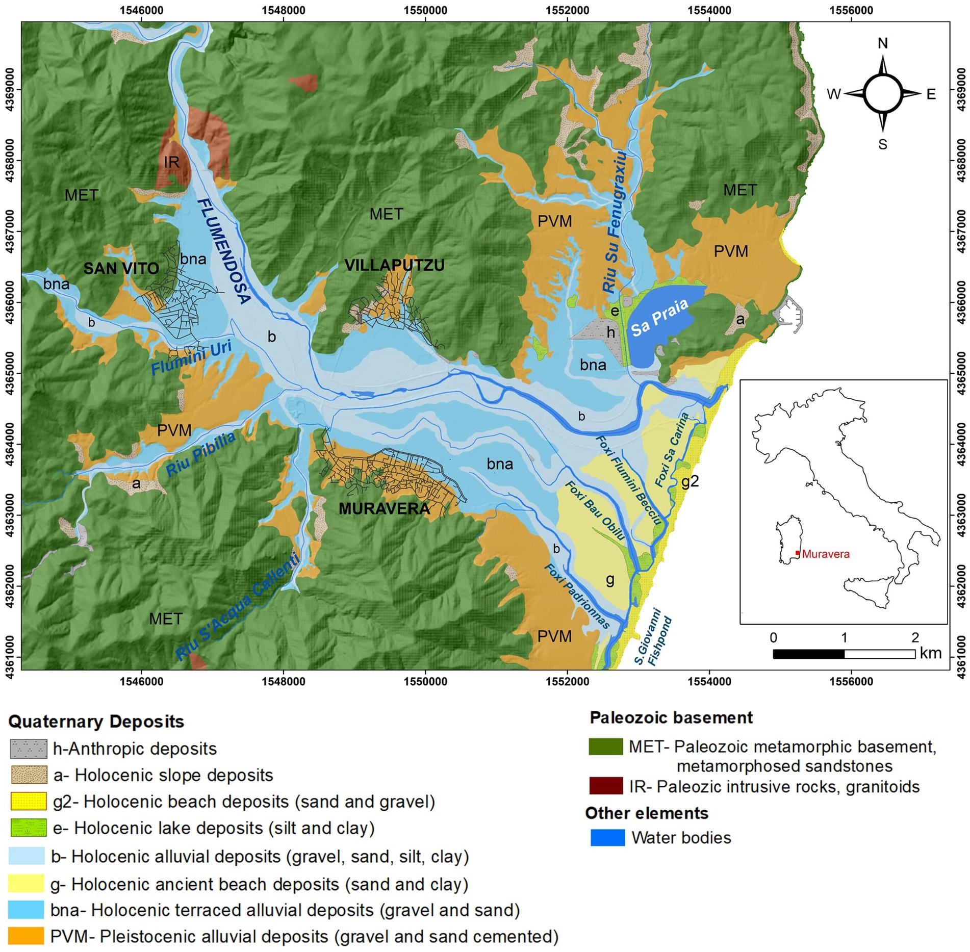
Figure 1. Geological map of the study area (Regione Autonoma della Sardegna, 2024). The coordinates on the horizontal and vertical axes are in meters. The coordinate system is a Transverse Mercator Projection (Monte Mario Italy 1).

2.2.1 Geological and hydrogeological settings

The Muravera coastal plain features a geological and hydrogeological setting characterized by Pleistocene and Holocene alluvium (Figure 1). This alluvial layer overlays the metamorphic and granitic Paleozoic bedrock at the plain’s edges. In the eastern part of the plain, the Paleozoic basement lies several hundred meters beneath the ground level, covered by overlying deposits. Moving upstream and aligning with the secondary hydrographic network, the basement approaches a few tens of meters below ground level. The foothills surrounding the plain are predominantly composed of clastic sediments (conoids) that merge with ancient alluvium near water courses as they descend. The river valley floor and the entire plain consist of recent and current alluvium. The Quaternary deposits of the Upper Pleistocene and the Holocene overlay the basement in the foothills, while the central-eastern region exhibits a coastal plain facies deposit. Below the Holocene alluvial deposits and in heteropic contact with the fans, a thick clayey succession interspersed with sandy and pebbly layers was recognized.

The hydrogeological structure is defined by a complex multilayer aquifer, hosted by the Holocene alluvium, partly phreatic and locally confined. This aquifer predominantly comprises loose coarse alluvial deposits, with high transmittivity, facilitating a generally high-water circulation due to primary porosity. In specific areas, the presence of a clayey body hydraulically separates the deposit, resulting in a phreatic groundwater aquifer and a locally confined deeper aquifer (Ardau and Barbieri, 2000; Porru et al., 2021). The piezometric head range approximately from 8 m above sea level (masl) in the north-western part of the plain to below zero towards the sea, with a medium gradient of 1‰. The conoids (Pleistocene continental deposits) host a low productive aquifer, with lower hydraulic conductivity and steeper hydraulic gradient (13‰).

2.2.2 Land Use

Part of the works carried out in this paper (namely, the SINTACS simulations) relies on a land use map, sourced from the Corine Land Cover 2008 database (Regione Autonoma della Sardegna, 2008), and updated by Porru et al. (2021), as shown in Figure 2. The area encompasses 18 diverse land-use classes such as water bodies, pastures, crops, orchards, and urban areas.

Figure 2

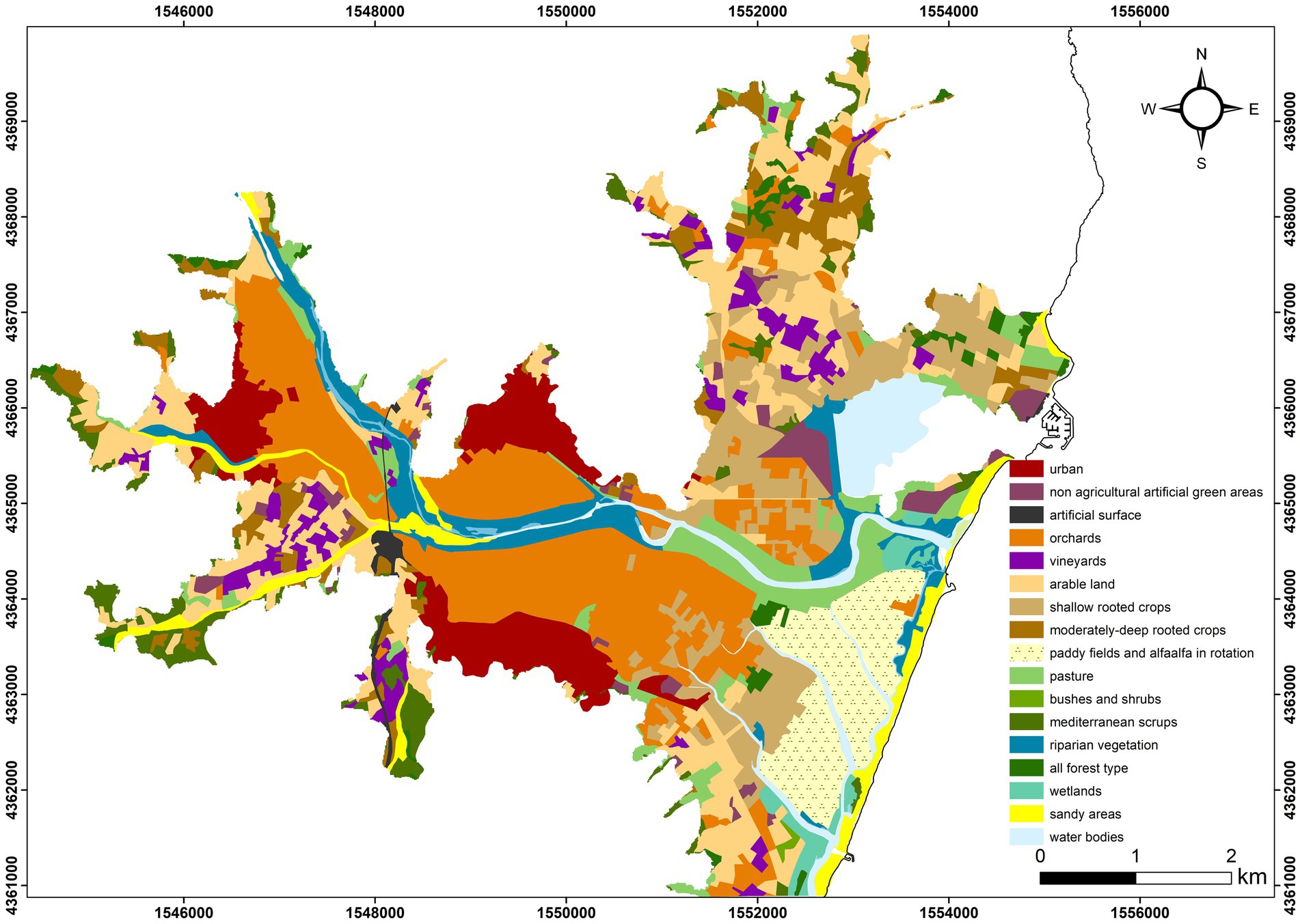
Figure 2. Land use map of the study area. The coordinates on the horizontal and vertical axes are in meters. The coordinate system is a Transverse Mercator Projection (Monte Mario Italy 1).

2.2.3 Soils

Figure 3 shows the distribution of prevailing soils in the study area. Most soils are derived from Holocene alluvial deposits and are characterized by a A-Bw-C horizon sequence and classified as Cambisols. These are deep soils, mostly with a texture class of loam, sandy loam, clay loam or sandy clay loam. Most of them show stratification due to the arrival of fresh material and have high base saturation (Eutric Fluvic Cambisols). In the areas closest to the coast, these soils are affected by salinity and sodicity [Eutric Fluvic Cambisols (Salic, Sodic)]. In these areas, soils with a surface horizon, or a subsurface horizon at a shallow depth, that contains high amounts of readily soluble salts, i.e., salts more soluble than gypsum, and sodicity may also occur (Sodic Solonchaks). In the highest Holocene alluvial terraces, Cambisols with low base saturation (Dystric Cambisols) can be found, while in the plain, whenever the arrival of fresh material is affecting the mineral soil surface, Eutric Fluvisols are found. Soils derived from Pleistocene alluvial deposits are characterized by a A-Bt-C horizon sequence and classified as Luvisols. These are deep soils, mostly with a texture class of sandy clay loam to clay loam. Soils derived from sand dunes and beaches are characterized by a A-C horizon sequence and a loamy sand or sand texture class and are classified as Eutric Arenosols.

Figure 3

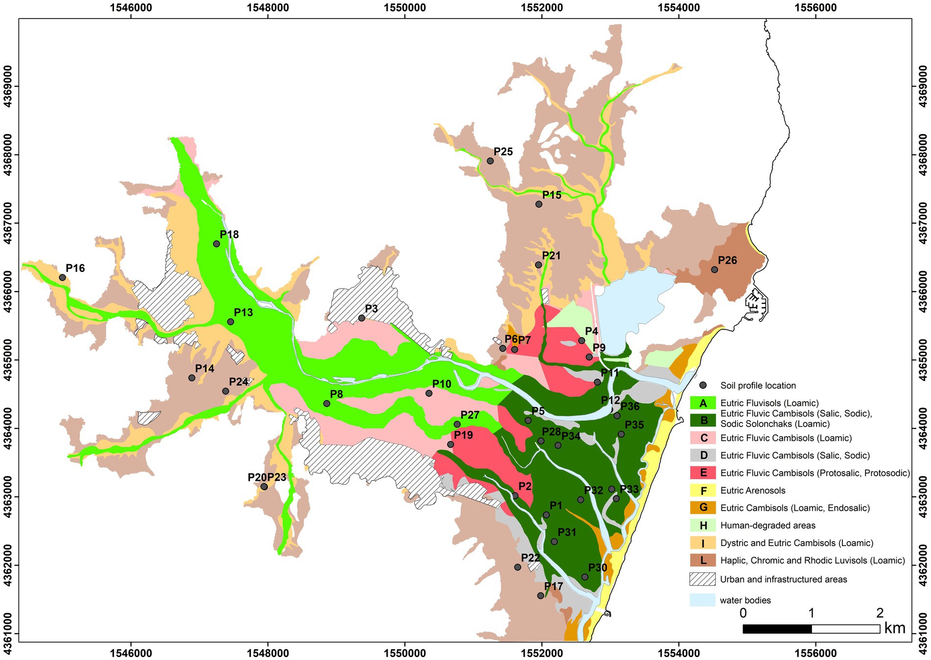
Figure 3. Distribution of prevailing soils in the study area (modified by AGRIS et al., 2014). The coordinates on the horizontal and vertical axes are in meters. The coordinate system is a Transverse Mercator Projection (Monte Mario Italy 1).

2.2.4 Soil texture, hydraulic and hydro-dispersive properties of the soil profiles examined

The soil data for the study area were sourced from the Database of Sardinia’s soils (AGRIS Sardinia Agency, Portale del suolo, http://dbss.sardegnaportalesuolo.it/, authorization required). This comprehensive dataset comprises soil information from 223 sites, with 187 specifically focusing on the surface layer (the Ap horizon) from 0 to 40 cm depth, and the remaining focusing on 36 soil profiles, each spanning two to six different horizons, with variables depths, from 60 to over 365 cm. The tabular soil data file encompasses a variety of morphological, physical, and chemical properties, including data on thickness, soil texture, available water capacity, and more.

In this investigation, raster layers for sand, silt, and clay were created using data from all 223 soil sites within the 40 cm surface layer. The ordinary Kriging interpolation method in GIS was applied to produce each raster layer, as depicted in Figure 4. This methodology provides a detailed representation of soil texture in the soil surface horizon across the study area.

Figure 4

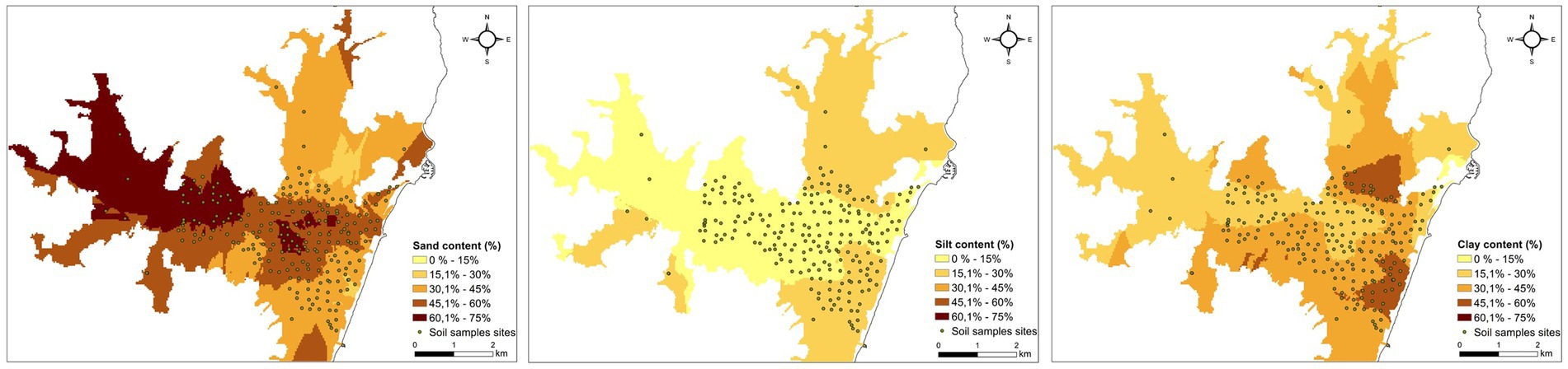
Figure 4. Sand, silt and clay content of the surface horizon produced by ordinary Kriging.

The pedotransfer function (PTF), known as ROSETTA (Schaap et al., 2001), was used for estimating soil hydraulic properties, leveraging the online resource provided at https://www.handbook60.org/rosetta/result. Within this study, the estimation of soil hydraulic properties was predicted on key factors such as soil texture, encompassing sand, silt, and clay percentages, along with bulk density, wilting point, and field capacity. This method expeditiously provides information for saturated water content, residual water content and the other shape parameters of the Mualem (1976) and van Genuchten (1980) unimodal soil water retention function and hydraulic conductivity.

To simulate solute transport, dispersivity (λ) values have also to be available for every soil horizon of each soil profile. As there were only limited measurements in the dataset for the area under study, we opted for deriving dispersivity values by applying the method proposed by Scotter and Ross (1994), which deduces breakthrough curves of a tracer at a given depth for a given soil starting by its hydraulic conductivity curve (Coppola et al., 2014; Bancheri et al., 2021).

2.2.5 Meteorological data, reference evapotranspiration, ETr, and rainfall

The daily reference evapotranspiration has been calculated by applying the FAO Penman-Monteith method $E{T}_r$ (Eq. 11).

$\begin{array}{ll}E{T}_r=\frac{0.408\mathrm{\Delta }\left(R_n-G\right)+\gamma \frac{900}{T+273}{u}_2\left(e_s-e_a\right)}{\mathrm{\Delta }+\gamma \left(1+0.34u_2\right)}& (11)\end{array}$

where $E{T}_r$ is the reference evapotranspiration (mm d⁻¹), $R_n$ the net radiation (MJ m⁻² d⁻¹), $\left(e_s-e_a\right)$ the difference between the saturation vapor pressure $e_s$ (KPa) and the actual vapor pressure $e_a$ (kPa), Δ the slope of the saturation vapor pressure–temperature curve (KPa °C ⁻¹), $\gamma$ the psychrometric constant (KPa °C⁻¹), $u_2$ the wind speed at 2 m height (m s⁻¹), T the mean daily air temperature (°C), and G the daily soil heat flux density (MJ m⁻² d⁻¹). For the calculation of the $E{T}_r$ by Eq. 1, the practical procedure proposed by Allen et al. (1998) was followed in this paper. The study collected daily meteorological data from the Villaputzu weather station for the years 2018 to 2023, accessible at https://stazionemeteovillaputzu.altervista.org/pages/station/table.php. The data included key parameters such as maximum and minimum temperature (°C), maximum and minimum relative humidity (%), average daily wind speed (m/s), maximum and minimum vapor pressure (KPa) and rainfall (mm). Table 1 provides an overview of annual climatic data for the years 2018 to 2023. Note the significantly high total annual rainfall of 1,092 mm in 2018.

Table 1

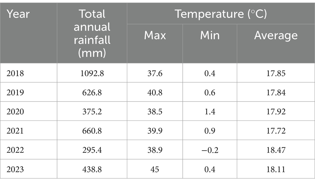
Table 1. Annual climatic data used for simulations.

Figure 5 illustrates a six-year time series of rainfall and evapotranspiration ( $E{T}_r$ ) using the data obtained from the Villaputzu weather station as mentioned above. The rainfall pattern displays significant temporal variability, with lower probabilities of rainfall during the summer. Furthermore, $E{T}_r$ reaches its maximum during the middle period of the year, specifically at the end of June to July.

Figure 5

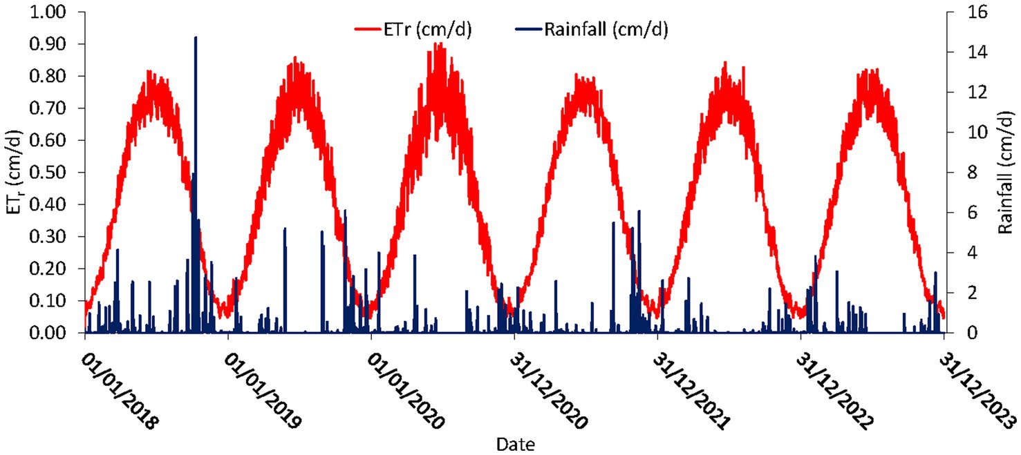
Figure 5. Daily measured rainfall and estimated reference evapotranspiration for the years 2018 to 2023.

2.2.6 Depth to groundwater

In this study, the groundwater serves a pivotal role as a potential bottom boundary condition. Porru (2023) monitored water level fluctuations in the Muravera Plain over a one-year period, spanning from June 2020 to May 2021, conducting a total of ten surveys across 80 observation wells and surface water points. The determination of average depth to groundwater levels over the entire area involved calculating the average depth to groundwater level for each observation point and producing groundwater raster surface layer using the ordinary interpolated Kriging method in ArcGIS.

2.3 Data handling

2.3.1 SINTACS: simulation and model input

For groundwater vulnerability assessment, according to the SINTACS method, the study area was partitioned into a grid of 10 × 10 square meters termed EFQs (Finite Square Elements). In this study, a raster was developed for each parameter, following the methodologies suggested in Civita and De Maio (2004), and using the data provided in Table 2. Figure 6 shows the maps of the score assignments for each parameter.

Table 2

Table 2. Description of sources of data used to assess the SINTACS intrinsic vulnerability.

Figure 6

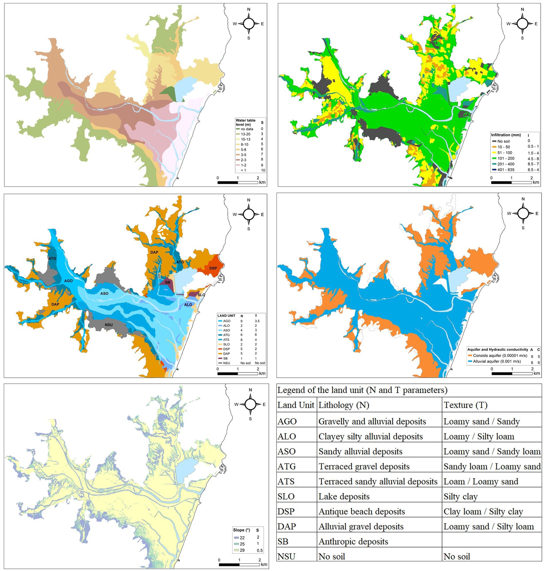
Figure 6. Maps indicating the score assignments for each parameter in SINTACS. The legend of the N and T parameter is reported separately in the table at the bottom right.

Using ESRI ArcGIS model builder, the raster of each parameter was multiplied by its corresponding weight from Table 2, overlaid, and used to calculate the vulnerability index. Since almost the entire study area is affected by agricultural activity (Figure 2) or occupied by urban settlements, the weights were assigned considering a scenario of relevant impact, adjusting the weight rating to emphasize the role of both the depth to water table and the unsaturated zone, as well as the fundamental function of soils. Relevant impact was used according to Civita and De Maio (2004), modifying the score assigned to hydraulic conductivity (parameter C), which was increased, and decreasing the weight of slope (parameter S), since the study area is flat. The application of the drainage scenario in river areas does not significantly alter the results. Therefore, only the weights of the relevant impact scenario are provided in Table 2.

2.3.2 FLOWS: numerical simulation and model inputs

Simulations with FLOWS were carried out by using the rainfall and reference evapotranspiration measured in the period 2018–2023 (for which a complete dataset was available). For the simulations, a complete set of hydraulic parameters (θ₀, θ_r, α_VG, n, K₀, τ = 0.5) were estimated by the PTF for each of the horizons of all the 36 soil profiles.

The length of the simulated flow field was established based on the depth to the groundwater. In the simulation sites where the depth to water table is deeper than 10 m, a simulation flow field length corresponding to the water table depth was considered, by assuming a zero-pressure head at the bottom boundary. In the sites where the depth to water table is larger than 10 m, we considered a flow field of 10 m, by assuming a unit gradient flow condition at the lower boundary.

In the first case, the simulation provided actual solute fluxes to groundwater and the solute travel times corresponded to the actual travel times to reach groundwater. In the second case, the breakthrough curve simulated at 10 m, along with the information on water fluxes and water contents at the same depth, were used to estimate travel times to groundwater. To do that, we did the following assumptions:

• steady state conditions (constant water contents and fluxes) were assumed in the deep vadose zone (from 10 m to the water table);

• the average water flux, $\overline{Jw}$ , and average water content $\overline{\theta }$ , at 10 m were calculated and used to obtain the average pore water velocity at the same depth as $\overline{v}=\overline{J_w}/\overline{\theta }$ ;

• by neglecting diffusion, $\overline{D_h}$ was calculated as $\lambda /\overline{v}$ (see Eq. 6).

• the dispersion coefficient, $\overline{D_h}$ , and the average pore water velocity, $\overline{v}$ , estimated at 10 m were used to calculate the travel time probability density function (TTf) at 10 m depth as:

$\begin{array}{ll}TTf\left(z,t\right)=\frac{z}{2\sqrt{\pi \overline{D_h}{t}^3}}exp\left[-\frac{{\left(z-\overline{v}t\right)}^2}{4\overline{D_h}t}\right]& (12)\end{array}$

the concentration breakthrough simulated at 10 m was considered as the input [C₀(t)] for the remaining part of the unsaturated zone (from 10 m to the GW table depth);

• Finally, the C₀(t) was convoluted through the TTf to obtain the breakthrough at the GW table according to the following equation (Jury and Roth, 1990; Bancheri et al., 2021):

$\begin{array}{ll}C\left(z,t\right)=\underset{0}{\overset{t}{{\displaystyle \int }}}{C}_0\left(0,t^{\prime }\right)TTf\left(z,t-t^{\prime }\right)d{t}^{\prime }& (13)\end{array}$

where $C_0\left(0,t^{\prime }\right)$ is the input concentration at 10 m depth (the breakthrough simulated by FLOWS at 10 m). These travel times were then added to the travel times from the soil surface to 10 m, calculated by FLOWS under transient conditions.

An inert, non-adsorbed (a tracer) solute was selected for simulation purposes. This was mainly because in this paper we were interested to predict the intrinsic vulnerability to pollution, that is where pollution is most likely to occur because of the physical system characteristics, independently on the potential impacts of specific land uses and chemico-dynamic properties of specific contaminants. The inert solute was applied at the top boundary as a 1-day specific area pulse of 10 g m⁻².

3 Results and discussions

3.1 SINTACS-based vulnerability analysis

The polygons in Figure 7 display the spatial distribution of the SINTACS-based vulnerability obtained for the Muravera plain. Vulnerability is characterized as high or very high across the entire plain, whereas it tends to be predominantly low or very low in areas corresponding to the conoids. In these areas, the depth to the water table is higher and the hydraulic conductivity of the aquifer is generally lower.

Figure 7

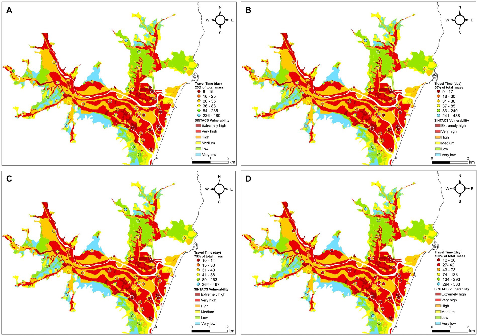
Figure 7. Map of groundwater vulnerability obtained by the SINTACS model. The dots indicate the vulnerability obtained by the FLOWS model in each of the soil profile. The figures A–D refer to the travel times for 25, 50, 75 and 100% specific mass arrival to the groundwater calculated by FLOWS.

3.2 SINTACS- and FLOWS-based vulnerability analyses

The soil profiles examined are characterized by diverse textural layers varying significantly in number, sequence, and thickness across profiles. The FLOWS model allowed addressing this complex vertical variability, by simulating water flow and solute transport individually for each profile, taking into consideration the local arrangement of textural layers. The simulation results were not condensed into vulnerability categories (e.g., low, medium, high), allowing for interpretation of local travel times based on specific conditions such as soil profile and water table depth. These simulation outputs were thus superimposed to the vulnerability map obtained by the SINTACS model (see Figures 7A–D). In the figure, all the four panels A, B, C and D depict the same continuous SINTACS vulnerability, whereas the circles indicate the travel time (in months) required for the 25 (TT25), 50 (TT50), 75 (TT75) and 100% (TT100) of the specific input mass (M₀ = 0.01 g/cm²) applied at the soil surface to reach the groundwater (GW). The data to build the maps are given in details in the Table 3, showing the solute travel times to the GW. For the profiles with deep GW table (> 10 m), the time required for the solute to reach the GW was estimated according to the procedure described in the section 2.7 (Data Handling: FLOWS: numerical simulations and model input).

Table 3

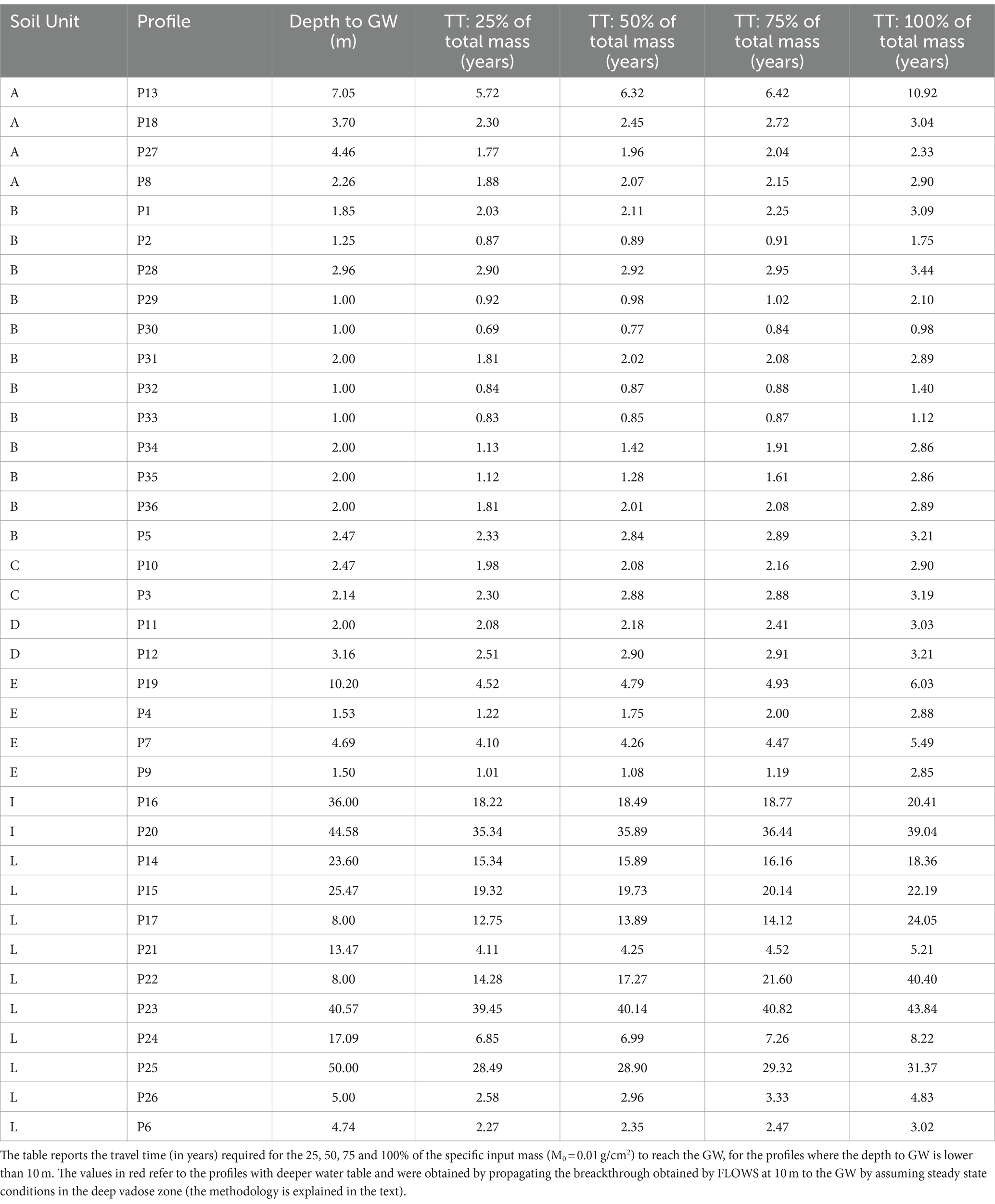
Table 3. Travel times to the groundwater (GW) for each of the soil profiles investigated.

The 25% arrival time of solute is crucial for evaluating environmental risks associated with contaminants that pose toxicity concerns at low concentrations (parts per million levels). In this context, this first arrival times solute may be more pertinent than the median transport (50%) times or the transport time for the whole mass (100%).

Upon examining the different maps, it is apparent that the two approaches provide consistent results, with high and low SINTACS groundwater vulnerability always corresponding to relatively low and high travel times, respectively. Also, the FLOWS-based travel times have consistent patterns for all the mass recovery values (i.e., 25, 50, 75 and 100% of solute mass), indicating that the variability of the dispersive behavior of the soil profiles do not alter enough the breakthrough curves so as to change the TT25, TT50, TT75 and TT100 patterns at the water table depth.

Depth to groundwater table, DGW, seems to have a large impact in determining the simulated travel times, as suggested by the graphs in the Figure 8, showing the relationship between the travel times simulated by FLOWS and DGW. The same may be said for the SINTACS, where DGW has a significant weight also in determining the vulnerability classes. The significant dependence of both model vulnerability results on DGW may thus well explain why the SINTACS and the FLOWS model gave coherent results. While this dependence was expected in the case of the SINTACS model, given the significant weight attributed to the DGW in identifying the SINTACS vulnerability classes, the same is not necessarily verified for the FLOWS model. In the latter, the dependence of travel times on the soil layering and hydrological properties (water retention, hydraulic conductivity, dispersivity) can be so strong that relatively higher travel times may be obtained even in presence of relatively shallow water table in the case of soil profiles with low hydraulic conductivity of the soil profile and vice versa. In other words, in the case of physically-based, dynamics approach specifically accounting for the vertical variability of the soil profile, such as FLOWS, the dependence of the travel times to the DGW cannot be always predicted a priori. This is the main reason why we used FLOWS as a parallel approach where the depth to groundwater is simply used as a physical and real bottom boundary condition to calculate travel times of pollutants to the groundwater. In this sense, the travel time approach allows for determining the extent of bias introduced by the depth to groundwater into the SINTACS results.

Figure 8

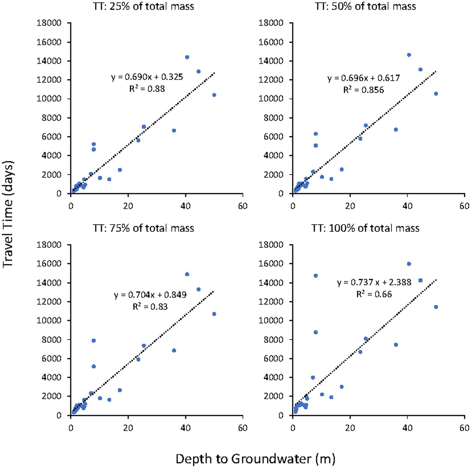
Figure 8. Relationship between travel times simulated by FLOWS and depth to groundwater. The three figures refer, respectively, to the 25, 50, 75 and 100 specific mass recovery. The figure also reports the R² for each of the three cases.

The graphs in Figure 8 show that the variability of travel times explained by the DGW (the correlation coefficient, R² in the graphs) decreases with increasing the recovered solute mass and data appear more scattered with increasing the DGW. In both cases, this behavior may be explained by the variability of the soil profiles (the depths and sequence of the layers in the profile, as well as their hydrological parameters), inducing quite different transport behavior (and thus travel times and shape of the breakthrough curves) even in the same soil unit. This is evident in the Figure 9, showing the whole set of cumulative breakthrough curves simulated by FLOWS at 1 m depth for all the soil profiles. In the graph, the thick red curve represents the average breakthrough curve.

Figure 9

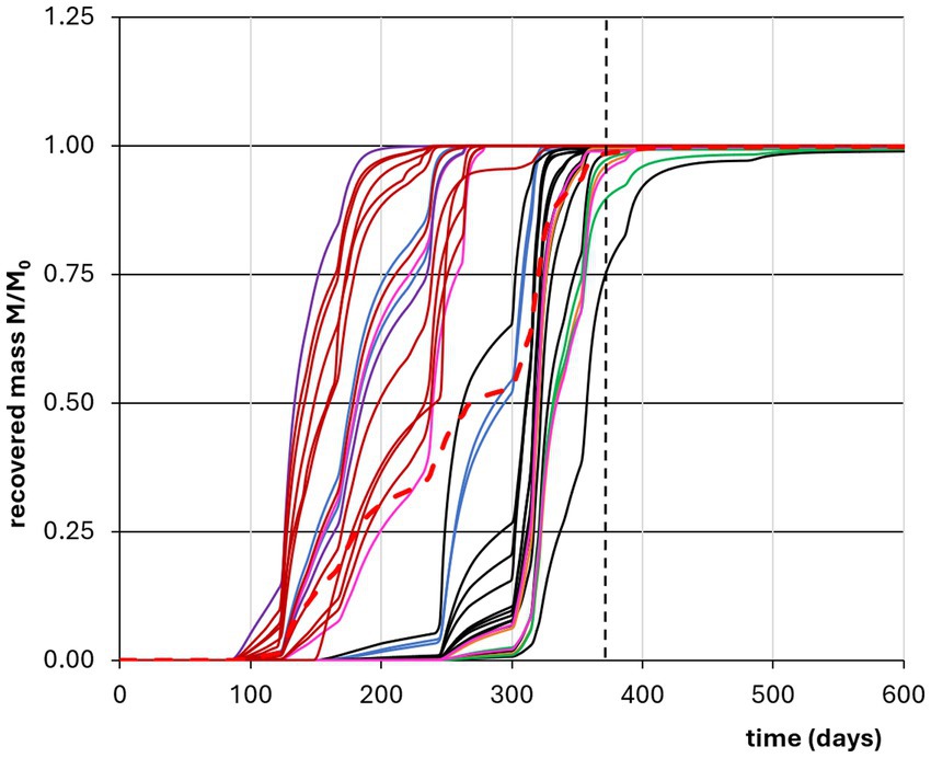
Figure 9. Whole set of cumulative breakthough curves at 1 m depth simulated by FLOWS for all the soil profiles investigated. The curves with the same color belong to the same soil unit. The thick red dashed curve represents the average curve.

By looking at the Figure 9, a large travel time variability may be already observed at 1 m depth, with 100% mass recovery travel times ranging from 200 to 500 days. However, these differences are not simply related to the fact that the soil profiles belong to different soil units. The graphs in Figure 10 show the same curves depicted in Figure 9 but divided for the different soil units. From the figures, it may be observed that quite different curves were obtained for the same soil unit, suggesting that even a macroscopic uniformity of soil profiles from a pedological point of view may result in significant changes in their hydrological behavior, with quite different hydraulic properties and dispersivities of the different soil layers. For the same reasons, it is even possible that soil profiles belonging to different soil units are characterized by similar breakthrough curves. Supplementary Table S1 provides the soil hydraulic parameters of each layer of each soil profile in the study area.

Figure 10

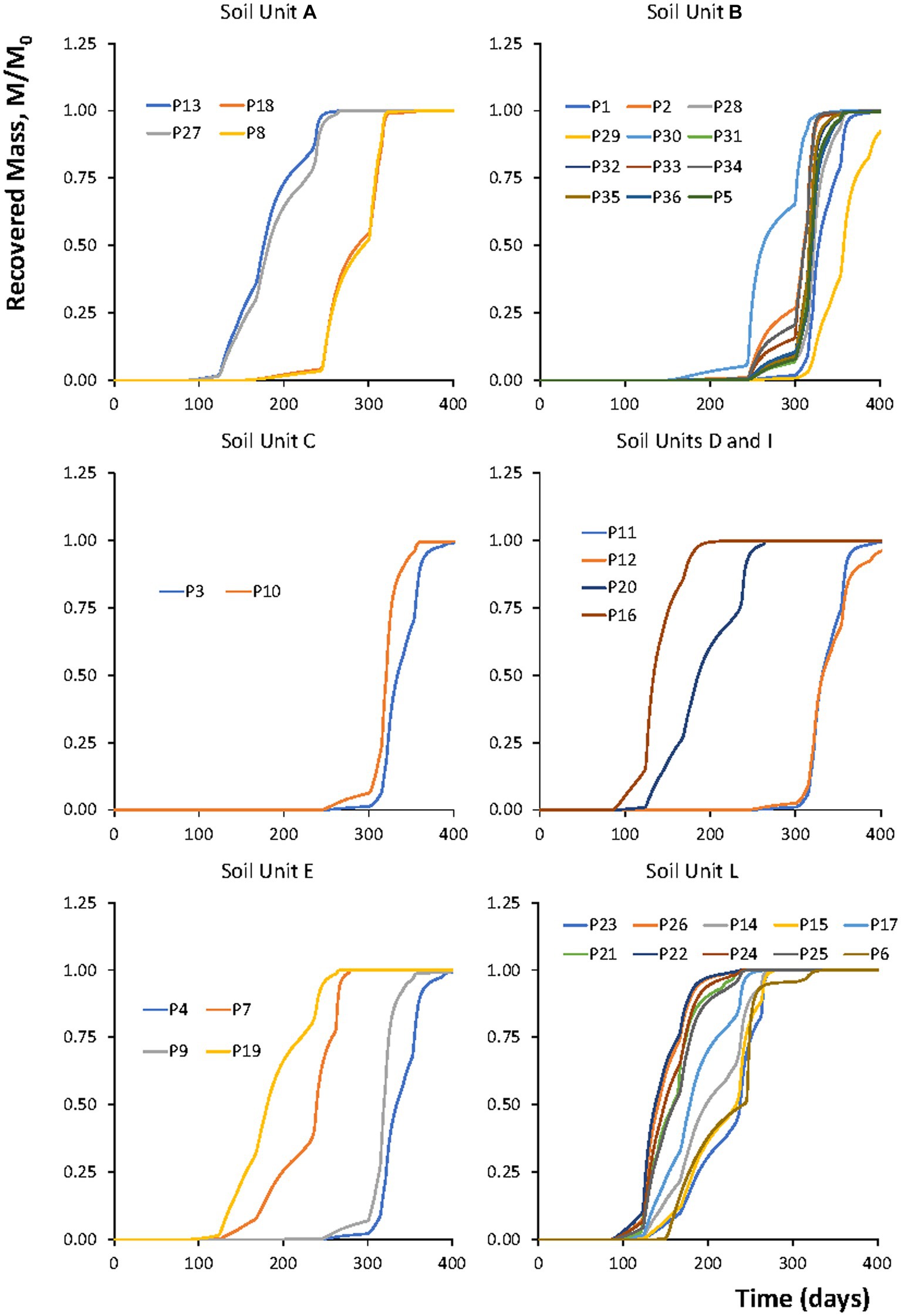
Figure 10. Breakthrough curves at 1 m depth for the same soil profiles shown in the previous figure, grouped by soil units.

The leverage analysis was carried out as explained in section 2.1.3 (Model comparison and validation) (see Figure 11). By looking at the figure, P25 had the highest leverage, P25 thus removed from the dataset used for correlation analysis. As an example, the graphs in Figure 8 were drawn again by removing the profile P25 and recalculating R² (Figure 12), to show that correlation was not significantly affected by removing the profile with the highest leverage.

Figure 11

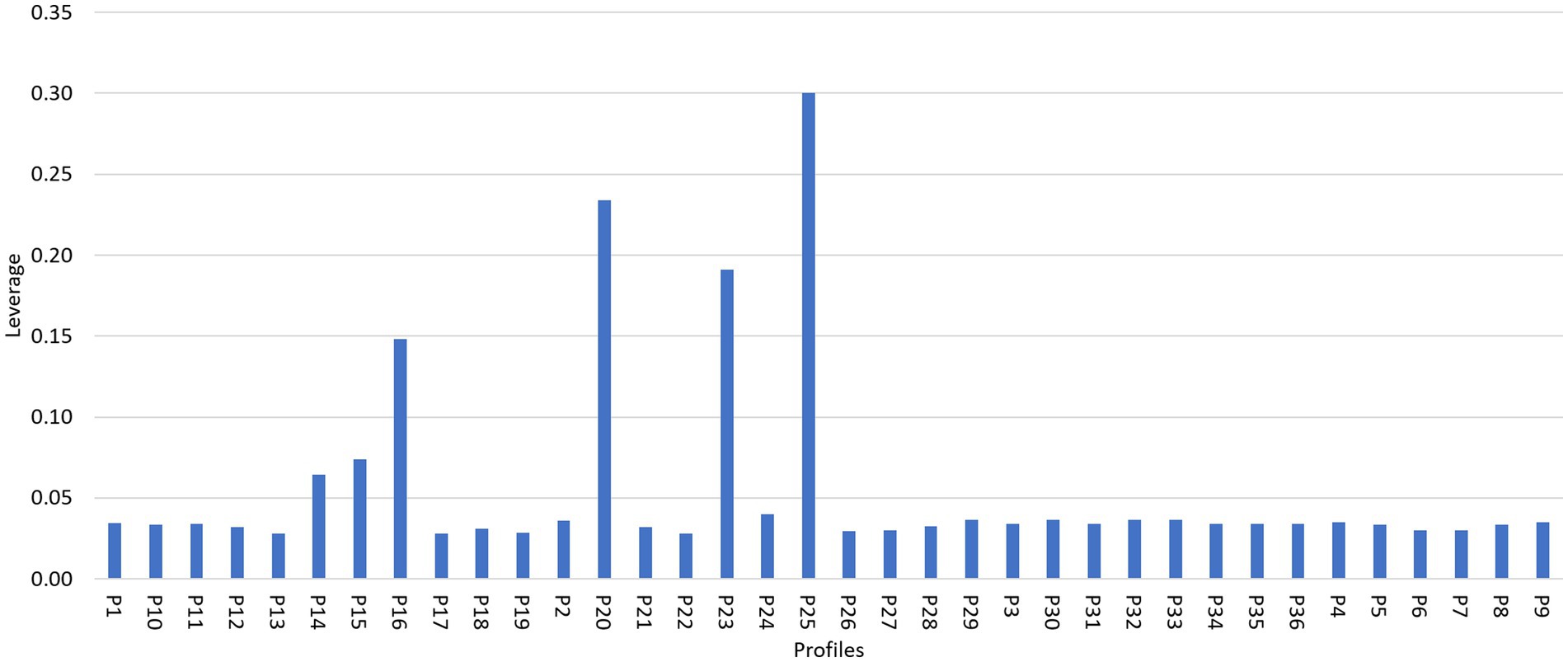
Figure 11. Leverage analysis results for each of the profiles to show their leverage in terms of the average depth to groundwater table, DGW.

Figure 12

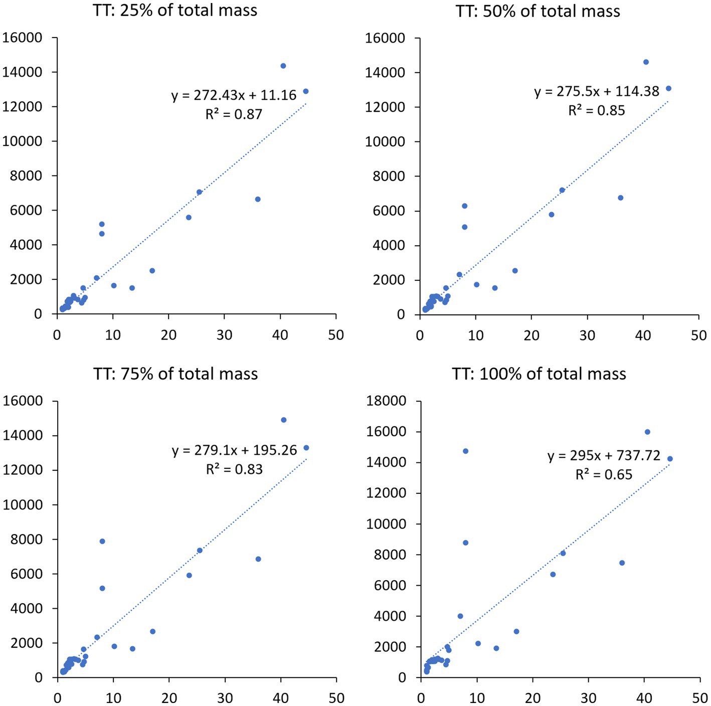
Figure 12. Relationship between travel times simulated by FLOWS and depth to groundwater for all the profiles except profile P25 which has the highest leverage as shown in Figure 11.

We also tried to validate the predicted vulnerability by analyzing the correlation between nitrate concentrations and travel times calculated by FLOWS. From the analysis, a poor correlation was found (see Supplementary Figure S1), which comes from the relatively uniform nitrate concentration in almost all the wells considered in this study (see nitrate concentrations in the map of Supplementary Figure S2). Nevertheless, to us, this result does not invalidate the model predictions. Actually, a uniform distribution of nitrate in the alluvial aquifer under study was largely expected due to its large transmissivity, which induces a relatively fast spreading of solutes once they reach the groundwater table and thus, relatively lower concentrations. By contrast, some relatively higher concentrations may be found in a few wells in the conoids, where the vulnerability is expected to be lower. This lack of correlation in the conoids may be explained by the much lower transmissivity and sufficiently strong oxidizing conditions (which is not accounted for in models like SINTACS or FLOWS), which are responsible for maintaining relatively higher concentrations of nitrates.

Rather, this discussion would prove that vulnerability model validation with measured data should be used with prudence, especially in high-transmissivity aquifers. In such cases, a sort of reciprocal benchmarking among models may be the only viable alternative to “validate” prediction models. Besides, the validation of travel times predictions based on nitrate concentrations should be considered with caution, by considering that FLOWS simulations, aiming at evaluating intrinsic vulnerability, did not take into account the amount and type of fertilizers applied in the study area, nor the nitrogen transformation processes.

4 Conclusion

The aim of this paper was using two approaches to assess groundwater vulnerability, namely the SINTACS and FLOWS models, in a sort of a reciprocal validation proof. In general, both the models provided coherent results, mostly because of the large impact of the depth to groundwater in determining both the rankings in the SINTACS map and the travel times in FLOWS simulations. On one side, this finding is an indirect proof of an adequate characterization of the physical system at study. Related to this, it also suggests that either conceptual or physically-based dynamics models may provide reliable results, even if with different spatial (and temporal) details, when an appropriate characterization of the physical system is available.

The main strength of this study was that it considered the integrated effects of spatial variation of soil profiles, and related soil physical properties, both in the vertical and horizontal dimensions. Our methodology addresses this issue by departing from the notion of modal soils and explicitly incorporates the actual vertical sequences of soil profiles and their spatial variability. However, while being a powerful tool in principle, this approach may only produce reliable results when large amounts of specific data are available. Results showed large differences in the magnitude of the different travel times among different profiles. The relatively lower or higher vulnerability was found to be mainly related to the depth to GW. However, this relationship weakens with increasing GW depth and solute mass to be recovered, indicating an increasing role of the soil variability for larger travel times, which cannot be identified by an overlay and index model, mostly based on conceptualizations of chemical transport, and thus providing general indication rankings of vulnerability.

Yet, as already mentioned in the Introduction section of this paper, one must acknowledge that the concept of vulnerability inherently carries some level of vagueness. It can only offer a relative indication of where contamination is more likely to occur and how it might progress spatially and temporally into groundwater. Both the approaches used in this paper keep some uncertainties, both have pros and cons. While overlay and index models identifies vulnerable macro-areas based on conceptualization of the physical system, including aquifer characteristics, physically based transient state hydrodynamic models are totally based on a detailed description of the travel times to the groundwater, which is important to reveal the impact of hydrological variability within soil units. Both are evidently incomplete and somehow complementary approaches.

Data availability statement

The original contributions presented in the study are included in the article/Supplementary material, further inquiries can be directed to the corresponding author.

Author contributions

MP: Data curation, Investigation, Visualization, Writing – review & editing. SH: Data curation, Formal analysis, Writing – review & editing. MA: Data curation, Visualization, Writing – review & editing. AV: Data curation, Investigation, Writing – review & editing. SD: Methodology, Validation, Writing – review & editing. AC: Conceptualization, Methodology, Software, Supervision, Writing – original draft.

Funding

The author(s) declare financial support was received for the research, authorship, and/or publication of this article. This study was partially carried out within the RETURN Extended Partnership and received funding from the European Union Next-Generation EU (National Recovery and Resilience Plan – NRRP, Mission 4, Component 2, Investment 1.3 – D.D. 1243 2/8/2022, PE0000005) and partly within the Agreement POA FSC 2014–2020 – 16.12.2019 among the ex MATTM-DGSTA and River Basin Authority (AdB) of Sardinia – Service for the protection and management of water resources, water services and drought management—Regional Agency of the River basin district of Sardinia, Action 2.3.1 “Interventions to improve the quality of water bodies”.

Conflict of interest

The authors declare that the research was conducted in the absence of any commercial or financial relationships that could be construed as a potential conflict of interest.

Publisher’s note

All claims expressed in this article are solely those of the authors and do not necessarily represent those of their affiliated organizations, or those of the publisher, the editors and the reviewers. Any product that may be evaluated in this article, or claim that may be made by its manufacturer, is not guaranteed or endorsed by the publisher.

Supplementary material

The Supplementary material for this article can be found online at: https://www.frontiersin.org/articles/10.3389/frwa.2024.1399170/full#supplementary-material

References

AGRIS, LAORE, Università degli Studi di Cagliari, Università degli Studi di Sassari. (2014). Carta delle Unità di Terre alla scala 1:50.000—Muravera-Villaputzu-Castiadas. http://www.sardegnaportalesuolo.it/cartografia/carte-dei-suoli/carta-delle-unita-di-terre-cut-alla-scala-150000.html (last accessed 19.02.2024).

Google Scholar

Allen, R. G., Pereira, L. S., Raes, D., and Smith, M. (1998). “Crop evapotranspiration: guidelines for computing crop requirements” in Irrigation and drainage paper no. 56 (Rome, Italy: FAO).

Google Scholar

Aller, L., and Thornhill, J. (1987) in DRASTIC: A standardized system for evaluating ground water pollution potential using hydrogeologic settings. ed. S. Robert (Ada, Oklahoma: Kerr Environmental Research Laboratory, Office of Research and Development, US Environmental Protection Agency).

Google Scholar

Ardau, F., and Barbieri, G. (2000). A quifer configuration and possible causes of salination in the Muravera plain (SE Sardinia, Italy). In Proc. of 16th salt water intrusion meeting, Miedzyzdroje-wo lin island, Polonia (11–18).

Google Scholar

Bancheri, M., Coppola, A., and Basile, A. (2021). A new transfer function model for the estimation of non-point-source solute travel times. J. Hydrol. 598:126157. doi: 10.1016/j.jhydrol.2021.126157

Crossref Full Text | Google Scholar

Biddau, R., Cidu, R., Da Pelo, S., Carletti, A., Ghiglieri, G., and Pittalis, D. (2019). Source and fate of nitrate in contaminated groundwater systems: assessing spatial and temporal variations by hydrogeochemistry and multiple stable isotope tools. Sci. Total Environ. 647, 1121–1136. doi: 10.1016/j.scitotenv.2018.08.007

PubMed Abstract | Crossref Full Text | Google Scholar

Bordbar, M., Rezaie, F., Bateni, S. M., Jun, C., Kim, D., Busico, G., et al. (2024). Global review of modification, optimization, and improvement models for aquifer vulnerability assessment in the era of climate change. Curr. Clim. Chang. Rep. 9, 45–67. doi: 10.1007/s40641-023-00192-2

Crossref Full Text | Google Scholar

Civita, M., and De Maio, M. (1997). SINTACS. Un sistema parametrico per la valutazione e la cartografia della vulnerabilita’ degli acquiferi all’inquinamento: Metodologia e Automatizzazione. Bologna (Italy): Pitagora Editrice.

Google Scholar

Civita, M., and De Maio, M. (2004). Assessing and mapping groundwater vulnerability to contamination: the Italian combined approach. Geofis. Int. 43, 513–532. doi: 10.22201/igeof.00167169p.2004.43.4.776

Crossref Full Text | Google Scholar

Comegna, V., Coppola, A., and Sommella, A. (1999). Nonreactive solute transport in variously structured soil materials as determined by laboratory-based time domain reflectometry (TDR). Geoderma 92, 167–184. doi: 10.1016/S0016-7061(99)00030-0

Crossref Full Text | Google Scholar

Coppola, A., Chaali, N., Dragonetti, G., Lamaddalena, N., and Comegna, A. (2015a). Root uptake under non-uniform root-zone salinity. Ecohydrology. (2014 8, 1363–1379. doi: 10.1002/eco.1594

Crossref Full Text | Google Scholar

Coppola, A., Comegna, V., Basile, A., Lamaddalena, N., and Severino, G. (2009). Darcian preferential water flow and solute transport through bimodal porous systems: experiments and modelling. J. Contam. Hydrol. 104, 74–83. doi: 10.1016/j.jconhyd.2008.10.004

PubMed Abstract | Crossref Full Text | Google Scholar

Coppola, A., Comegna, A., Dragonetti, G., Gerke, H. H., and Basile, A. (2015b). Simulated preferential water flow and solute transport in shrinking soils. Vadose Zone J. 14, 1–22. doi: 10.2136/vzj2015.02.0021

Crossref Full Text | Google Scholar

Coppola, A., Dragonetti, G., Comegna, A., Zdruli, P., Lamaddalena, N., Pace, S., et al. (2014). Mapping solute deep percolation fluxes at regional scale by integrating a process-based vadose zone model in a Monte Carlo approach. Soil Sci. Plant Nutr. 60, 71–91. doi: 10.1080/00380768.2013.855615

Crossref Full Text | Google Scholar

Coppola, A., Dragonetti, G., Sengouga, A., Lamaddalena, N., Comegna, A., Basile, A., et al. (2019). Identifying optimal irrigation water needs at district scale by using a physically based agro-hydrological model. Water 11:841. doi: 10.3390/w11040841

Crossref Full Text | Google Scholar

Coppola, A., Gerke, H. H., Comegna, A., Basile, A., and Comegna, V. (2012). Dual-permeability model for flow in shrinking soil with dominant horizontal deformation. Water Resour. Res. 48:W08527. doi: 10.1029/2011WR011376

Crossref Full Text | Google Scholar

Coppola, A., and Randazzo, L. (2006). “A MathLab code for the transport of water and solutes in unsaturated soils with vegetation, technical report” in Soil and Contam (Potenza, Italy: Hydrol. Lab., Dep. DITEC, Univ. of Basilicata).

Google Scholar

Corwin, D. L., Vaughan, P. J., and Loague, K. (1997). Modeling non-point source pollutants in the vadose zone with GIS. Environ. Sci. Technol. 31, 2157–2175. doi: 10.1021/es960796v

Crossref Full Text | Google Scholar

Fusco, F., Allocca, V., Bancheri, M., Basile, A., Calcaterra, D., Coppola, A., et al. (2024). A multi-method approach for assessing groundwater vulnerability of shallow aquifers in the Marchfeld region (Austria). J. Hydrol. Reg. Stud. 54:101865. doi: 10.1016/j.ejrh.2024.101865

Crossref Full Text | Google Scholar

Gogu, R. C., and Dassargues, A. (2000). Current trends and future challenges in groundwater vulnerability assessment using overlay and index methods. Environ. Geol. 39, 549–559. doi: 10.1007/s002540050466

Crossref Full Text | Google Scholar

Hassan, S. B. M., Dragonetti, G., Comegna, A., Lamaddalena, N., and Coppola, A. (2023). Analyzing the role of soil and vegetation spatial variability in modelling hydrological processes for irrigation optimization at large scale. Irrig. Sci. 42, 249–267. doi: 10.1007/s00271-023-00882-7

Crossref Full Text | Google Scholar

Hassan, S. B. M., Dragonetti, G., Comegna, A., Sengouga, A., Lamaddalena, N., and Coppola, A. (2022). A bimodal extension of the ARYA and PARIS approach for predicting hydraulic properties of structured soils. J. Hydrol. 610:127980. doi: 10.1016/j.jhydrol.2022.127980

Crossref Full Text | Google Scholar

Jahromi, M. N., Gomeh, Z., Busico, G., Barzegar, R., Samany, N. N., Aalami, M. T., et al. (2021). Developing a SINTACS-based method to map groundwater multi-pollutant vulnerability using evolutionary algorithms. Environ. Scien. Pollut. Res. 28, 7854–7869. doi: 10.1007/s11356-020-11089-0

PubMed Abstract | Crossref Full Text | Google Scholar

Jain, H. (2023). Groundwater vulnerability and risk mitigation: a comprehensive review of the techniques and applications. Groundw. Sustain. Dev. 22:100968. doi: 10.1016/j.gsd.2023.100968

Crossref Full Text | Google Scholar

Jury, W. A., and Roth, K. (1990). Transfer functions and solute movement through soil: theory and applications. Basel: Birkhauser Verlag AG.

Google Scholar

Jury, W. A., Spencer, W. F., and Farmer, W. J. (1983). Behavior assessment model for trace organics in soil: I. Model description. J. Environ. Qual. 12, 558–564. doi: 10.2134/jeq1983.00472425001200040025x

Crossref Full Text | Google Scholar

Kanter, D. R., and Brownlie, W. J. (2019). Joint nitrogen and phosphorus management for sustainable development and climate goals. Environ. Sci. Pol. 92, 1–8. doi: 10.1016/j.envsci.2018.10.020

Crossref Full Text | Google Scholar

Kanter, D. R., Chodos, O., Nordland, O., Rutigliano, M., and Winiwarter, W. (2020). Gaps and opportunities in nitrogen pollution policies around the world. Nat. Sustain. 3, 956–963. doi: 10.1038/s41893-020-0577-7

Crossref Full Text | Google Scholar

Lawniczak, A. E., Zbierska, J., Nowak, B., Achtenberg, K., Grześkowiak, A., and Kanas, K. (2016). Impact of agriculture and land use on nitrate contamination in groundwater and running waters in central-West Poland. Environ. Monit. Assess. 188, 172–117. doi: 10.1007/s10661-016-5167-9

PubMed Abstract | Crossref Full Text | Google Scholar

Masroor, M., Rehman, S., Sajjad, H., Rahaman, M. H., Sahana, M., Ahmed, R., et al. (2021). Assessing the impact of drought conditions on groundwater potential in Godavari middle Sub-Basin, India using analytical hierarchy process and random forest machine learning algorithm. Groundw. Sustain. Dev. 13:100554. doi: 10.1016/j.gsd.2021.100554

Crossref Full Text | Google Scholar

McCoy, N., Chao, B., and Gang, D. D. (2015). Nonpoint source pollution. Water Environ. Res. 87, 1576–1594. doi: 10.2175/106143015X14338845156263

Crossref Full Text | Google Scholar

Moraru, C., and Hannigan, R. (2018). Analysis of hydrogeochemical vulnerability. Cham, Switzerland: Springer International Publishing.

Google Scholar

Mualem, Y. (1976). A new model for predicting the hydraulic conductivity of unsaturated porous media. Water Resour. Res. 12, 513–522. doi: 10.1029/WR012i003p00513

Crossref Full Text | Google Scholar

Nolan, B. T., Hitt, K. J., and Ruddy, B. C. (2002). Probability of nitrate contamination of recently recharged groundwaters in the conterminous United States. Environ. Sci. Technol. 36, 2138–2145. doi: 10.1021/es0113854

PubMed Abstract | Crossref Full Text | Google Scholar

Nolan, B. T., Ruddy, B. C., Hitt, K. J., and Helsel, D. R. (1997). Risk of nitrate in groundwaters of the United States: a national perspective. Environ. Sci. Technol. 31, 2229–2236. doi: 10.1021/es960818d

Crossref Full Text | Google Scholar

Porru, M. C. (2023). Caratterizzazione idrogeologica avanzata dell’acquifero alluvionale della piana costiera di Muravera. [PhD dissertation]. Cagliari (Italy): University of Cagliari.

Google Scholar

Porru, M. C., Arras, C., Biddau, R., Cidu, R., Lobina, F., Podda, F., et al. (2024). Assessing recharge sources and seawater intrusion in coastal groundwater: a hydrogeological and multi-isotopic approach. Water 16:1106. doi: 10.3390/w16081106

Crossref Full Text | Google Scholar

Porru, M. C., Da Pelo, S., Westenbroek, S., Vacca, A., Loi, A., Melis, M. T., et al. (2021). A methodological approach for the effective infiltration assessment in a coastal groundwater. Italian J. Eng. Geol. Environ. 1, 183–193. doi: 10.4408/IJEGE.2021-01.S-17

Crossref Full Text | Google Scholar

Rao, P. S. C., Hornsby, A. G., and Jessup, R. E. (1985). Indices for ranking the potential for pesticide contamination of groundwater. Soil Crop Sci. Soc. Fl. 44, 1–8.

Google Scholar

Regione Autonoma della Sardegna. (2008). Corine Land Cover: Carta dell’uso del suolo. Available at: https://www.sardegnageoportale.it/index.php?xsl=2420&s=40&v=9&c=14480&es=6603&na=1&n=100&esp=1&tb=14401 (Accessed May 31, 2024)

Google Scholar

Regione Autonoma della Sardegna. (2024). Available at: https://www.sardegnageoportale.it/

Google Scholar

Ritchie, J. T. (1972). Model for predicting evaporation from a row crop with incomplete cover. Water Resour. Res. 8, 1204–1213. doi: 10.1029/WR008i005p01204

Crossref Full Text | Google Scholar

Schaap, M. G., Leij, F. J., and van Genuchten, M. T. (2001). ROSETTA: a computer program for estimating soil hydraulic parameters with hierarchical pedotransfer functions. J. Hydrol. 251, 163–176. doi: 10.1016/S0022-1694(01)00466-8

Crossref Full Text | Google Scholar

Scotter, D. R., and Ross, P. J. (1994). The upper limit of solute dispersion and soil hydraulic properties. Soil Sci. Soc. Am. J. 58, 659–663. doi: 10.2136/sssaj1994.03615995005800030004x

Crossref Full Text | Google Scholar

Selim, H. M., and Amacher, M. C. (1996). Reactivity and transport of heavy metals in soils. New York: CRC Press.

Google Scholar

Severino, G., Comegna, A., Coppola, A., Sommella, A., and Santini, A. (2010). Stochastic analysis of a field-scale unsaturated transport experiment. Adv. Water Resour. 33, 1188–1198. doi: 10.1016/j.advwatres.2010.09.004

Crossref Full Text | Google Scholar

Stewart, I. T., and Loague, K. (2003). Development of type transfer functions for regional-scale non-point source groundwater vulnerability assessments. Water Res. Res. 39:1359. doi: 10.1029/2003WR002269

Crossref Full Text | Google Scholar

Troldborg, L., Jensen, K. H., Engesgaard, P., Refsgaard, J. C., and Hinsby, K. (2008). Using environmental tracers in modeling flow in a complex aquifer system. J. Hydrol. Eng. 13, 1037–1048. doi: 10.1061/(ASCE)1084-0699(2008)13:11(1037)

Crossref Full Text | Google Scholar

United Nations Environment Programme/Mediterranean Action Plan and Plan Bleu (2020). “State of the environment and development in the Mediterranean” in Chapter 6: Food and water security. Tunis Cedex - Tunisia: Specially Protected Areas Regional Activity Centre (SPA/RAC)

Google Scholar

van Dam, J. C. (2000). Field-scale water flow and solute transport: SWAP model concepts, parameter estimation and case studies. [doctoral thesis]. Wageningen (Netherlands): Wageningen University and Research.

Google Scholar

van Dam, J. C., Huygen, J., Wesseling, J. G., Feddes, R. A., Kabat, P., Van Walsum, P. E. V., et al. (1997). Theory of SWAP version 2.0; simulation of water flow, solute transport and plant growth in the soil-water-atmosphere-plant environment. Wageningen (Netherlands): DLO Winand Staring Centre.

Google Scholar

van Genuchten, M. T. (1980). A closed-form equation for predicting the hydraulic conductivity of unsaturated soils. Soil Sci. Soc. Am. J. 44, 892–898. doi: 10.2136/sssaj1980.03615995004400050002x

Crossref Full Text | Google Scholar

Vanderborght, J., and Vereecken, H. (2007). Review of dispersivities for transport modeling in soils. Vadose Zone J. 6, 29–52. doi: 10.2136/vzj2006.0096

Crossref Full Text | Google Scholar

Vereecken, H., Weynants, M., Javaux, M., Pachepsky, Y., Schaap, M. G., and van Genuchten, M. T. (2010). Using Pedotransfer functions to estimate the van Genuchten–Mualem soil hydraulic properties: a review. Vadose Zone J. 9, 795–820. doi: 10.2136/vzj2010.0045

Crossref Full Text | Google Scholar

Vogel, T. (1987). SWM II-numerical model of two-dimensional flow in a variably saturated porous medium. Research report no. 87,. The Netherlands: Department of Hydraulics and Catchment Hydrology, Agriculture University Wageningen.

Google Scholar

Vrba, J., and Zaporozec, A. (1994). Guidebook on mapping groundwater vulnerability. Hannover, Germany: Heise.

Google Scholar

Wang, T., Zlotnik, V. A., Simunek, J., and Schaap, M. G. (2009). Using pedotransfer functions in vadose zone models for estimating groundwater recharge in semiarid regions. Water Resour. Res. 45:W04412. doi: 10.1029/2008WR006903

Crossref Full Text | Google Scholar

Wösten, J. H. M., Pachepsky, Y. A., and Rawls, W. J. (2001). Pedotransfer functions: bridging the gap between available basic soil data and missing soil hydraulic characteristics. J. Hydrol. 251, 123–150. doi: 10.1016/S0022-1694(01)00464-4

Crossref Full Text | Google Scholar

Xepapadeas, A. (2011). The economics of non-point-source pollution. Annu. Rev. Resour. Econ. 3, 355–373. doi: 10.1146/annurev-resource-083110-115945

Crossref Full Text | Google Scholar

Yuan, L., Sinshaw, T., and Forshay, K. J. (2020). Review of watershed-scale water quality and nonpoint source pollution models. Geosciences 10, 25–36. doi: 10.3390/geosciences10010025

PubMed Abstract | Crossref Full Text | Google Scholar