Predictive uncertainty analysis for a highly parameterized karst aquifer using null-space Monte Carlo

Inverse problems in hydrogeology pose a great challenge for modelers as they are ill-posed, resulting in a non-unique solution. High computational resources are needed for the calibration process, especially in the case of highly parameterized aquifers like karst limestone, characterized by significant heterogeneity. The null-space Monte Carlo (NSMC) is a parameter-constrained Monte Carlo approach that can be used to quantify uncertainty, as it produces a set of solutions that calibrate the model. This method is used to assess uncertainty in the calibration of a karst aquifer in Qatar, which has high heterogeneity. Pilot points were used to reflect the geostatistics of the calibrated field, and the calibration results at these points were interpolated over the aquifer area using kriging. The NSMC was then used to produce 200 realizations of the null-space parameter field using the constrained random variable of hydraulic conductivity. The null-space realizations were then incorporated into the parameter space derived from the calibrated model. Statistical analysis of the calibrated hydraulic conductivity revealed a variation ranging from 0.1 to 350 m/d, indicating a considerable variability in the aquifer’s hydraulic parameters. The areas with high hydraulic conductivity were concentrated in the central and eastern parts of the aquifer, and these same areas exhibited a high standard deviation. Based on the findings of this study, while the NSMC method is effective for uncertainty analysis in solving inverse problems, it is important to note that a considerable number of runs are necessary to reach the threshold of calibration error. This is because of the significant non-linearity inherent in the karst aquifer.

1 Introduction

Karst carbonate aquifers display significant variability owing to the prevalence of numerous fractures and conduits within them. On the one hand, conducting an extensive series of field pumping tests for comprehensive heterogeneity characterization is not only expensive but also impractical. On the other hand, stochastic analysis demands a large number of simulations, incurring high computational costs. Calibrating models of groundwater flow in fractured porous media is even more challenging as the number of runs to solve the inverse problem is very high compared to the forward problems, demanding a computational effort that is often impractical. In cases of highly parameterized aquifers such as karst carbonate, conventional uncertainty methods can be challenging (Beven and Binley, 1992).

Several stochastic methods, such as Monte Carlo (MC) and its variants, have been used to cope with uncertainty in hydrogeology (Harvey and Gorelick, 1995; Baalousha, 2009; Hassan et al., 2009; Wu and Zeng, 2013; Ren et al., 2016). The problem with the MC approach is the high number of realizations required, which results in high computational expenses. The Monte Carlo approach has a slow convergence rate that is inversely proportional to the number of realizations (Owen, 1992; Baalousha, 2009). Latin hypercube sampling (LHS) is a modified method of classical Monte Carlo and is used to create a nearly random realization of parameters of interest. It was first introduced by Mckay et al. (1979) and later modified by Iman et al. (1981). In contrast to the Monte Carlo method, LHS partitions the sampling space into equal probable sub-spaces, placing one sample within each sub-space. This is the reason why it is referred to as controlled random sampling. LHS significantly reduces the required runs to achieve the same accuracy compared to Monte Carlo, and the variance is smaller (Owen, 1992; Hardyanto and Merkel, 2007). This method has been widely used in various uncertainty problems in hydrogeology and experiment design (Baalousha, 2006; Amini et al., 2008; Baalousha, 2009).

The population of hydraulic fields in x and y directions, even with a low number of LHS spaces, results in a significant increase in the required number of runs. Although LHS substantially reduces the number of runs needed to achieve results comparable to Monte Carlo, the computational cost for solving inverse problems remains prohibitively high, rendering its practical application challenging. Tonkin and Doherty (2009) presented the null-space Monte Carlo (NSMC) method for uncertainty analysis of model calibration. The NSMC is a practical approach to quantifying model calibration uncertainty, as it is model-independent and requires a small number of iterations (Doherty, 2015). As the calibration problem is ill-posed, the resulting calibrated field is non-unique (Carrera et al., 2005). NSMC enables the generation of diverse solutions, all of which calibrate the model. This capability facilitates the assessment of uncertainty associated with the calibrated variable. The NSMC approach has been successfully used to assess the uncertainty of various problems, such as saltwater intrusion, flow modeling, particle tracking, and remediation effectiveness (Sepulveda and Doherty, 2015; Formentin et al., 2019; Moeck et al., 2020). The pilot points approach is employed in model calibration as it is a middle ground between the cellwise representation of parameter variability and the zonation approach, which represents the entire domain through a few zones. In the case of high parametrization of heterogeneous aquifers, the pilot points approach is more suitable than zonation or full parametrization. Thus, the pilot points approach provides a smoother representation of the calibrated parameter field and reduces computational expenses (RamaRao et al., 1995; Doherty et al., 2011; Baalousha et al., 2019; Tziatzios et al., 2021).

Using random values within the parameter range, NSMC uses the null space to generate sets of parameters that match the field data. This randomness contributes to the method’s ability to explore the solution space.

The NSMC approach begins with the calibration of the model using mathematical regularization (singular value decomposition, SVD). Then, the null space of the parameter field is obtained using the parameter sensitivities (i.e., the Jacobian matrix), which is the partial derivative matrix of independent variables. The null space includes groups of parameters that we cannot obtain from observational data. Following this, many realizations of parameter fields are created. Each stochastic parameter set comprises null and solution space projections. The difference between each realization and the calibrated parameter (from the calibrated model) is obtained using the covariance of the variogram and projected into the null space. The null space comprises parameters that exert no influence on the outputs of the model despite variability in the dependent variable. Consequently, these parameter combinations can be integrated into any parameter set that successfully calibrates the model within the preset threshold error, resulting in an alternative set of parameters that also achieve effective calibration (Tonkin and Doherty, 2009). All these steps are done using the Parameter Estimation and Uncertainty Analysis Software (PEST) developed by Doherty (2015). In some cases, the model behavior is linear, and as such, the resulting obtained random field calibrates the model. However, in many cases, the model is non-linear, and in this case, the calibration error is not acceptable, and it requires a few iterations to be calibrated (Tonkin and Doherty, 2009). This study aimed to explore the effectiveness of employing NSMC to assess predictive uncertainty in inverse parameter estimates (the calibration process) for a highly parameterized aquifer. The calibration of such aquifers is particularly challenging due to their high heterogeneity. An aquifer in Qatar was used as a case study, chosen for its characteristics as a karstified carbonate aquifer.

2 Study area

Qatar is a member of the Gulf Cooperation Council (GCC) and spans in a north–south direction. It constitutes a peninsula surrounded by the Arabian Gulf on all sides, with its sole land border situated to the south, shared with Saudi Arabia (Figure 1). The primary source of natural water in Qatar is the northern aquifer, known for its good-quality water. This is attributed to favorable hydrogeological conditions, including high recharge rates and geology. The northern aquifer constitutes slightly less than half of Qatar’s total land area, covering an area of 4,300 km². The southern aquifer lies to the south of Qatar and is characterized by poor groundwater quality. This inferior quality is linked to the presence of gypsum in the subsurface, which dissolves in water and contributes to its deterioration. In contrast, the northern aquifer lacks these gypsum layers in its geological setting.

Figure 1

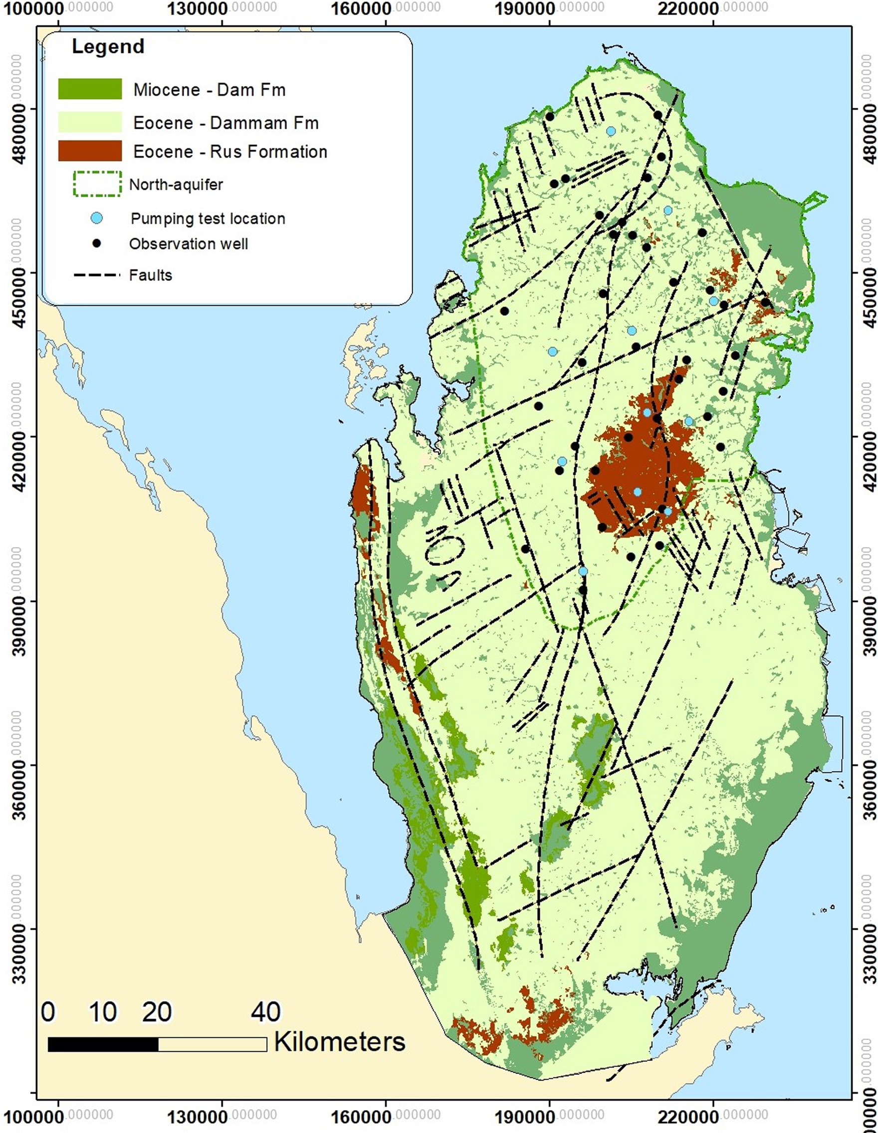
Figure 1. Map of Qatar showing the study area (north-aquifer), geology, and pumping test locations. Coordinate system is Qatar National Grid.

The aquifer receives its essential recharge from rainfall, which amounts to an annual average of less than 80 mm (Eccleston et al., 1981; Baalousha et al., 2021, 2023). Despite this low rainfall, recharge takes place as point sources in land depressions, where runoff accumulates and eventually replenishes the aquifer (Eccleston et al., 1981; Schlumberger Water Services, 2009; Baalousha et al., 2022).

The geology of the northern aquifer comprises various layers of carbonate deposits (Figure 1). The uppermost layer is the Miocene Dam Formation, which covers only smaller parts of Qatar and does not constitute an aquifer as it is mostly dry. The second layer is the Eocene Dammam Formation, which covers the majority of the land surface in Qatar. The third layer is a limestone and dolomite layer from the early Eocene Rus Formation. The evaporite layer of gypsum occurs within this layer in the southern half of Qatar. This layer hosts the evaporite gypsum layer found in the southern aquifer. The fourth and bottom layer is the lower Eocene Umm Al-Radhuma Formation, comprising dolomite and limestone (Vecchioli, 1976; Eccleston et al., 1981; Kimrey, 1985; Alsharhan et al., 2001). The latter formation does not outcrop on the surface. These Dammam, Rus, and Um Al-Radhuma collectively form the northern aquifer, with a thickness varying between 50 and 300 m (Al-Hajari, 1990; Jacob et al., 2021).

The aquifer is karstified, marked by numerous sinkholes, land depressions, and conduits, leading to significant variability in hydraulic properties (Baalousha, 2016a). The results of 11 aquifer tests (Figure 1) indicate that the transmissivity of the northern aquifer varies widely, ranging from 2.6 to 1,420 m²/d (Schlumberger Water Services, 2009). This extensive variability underscores the high heterogeneity of the aquifer.

3 Materials and methods

3.1 Methodology

Figure 2 depicts the stepwise methodology of this study. The approach starts with model input data for a forward model (box 1), which is run successfully. Next, for the calibration process, observation data and pumping test data are used (box 3a and box 3b), and the pilot points approach is employed, where a finite number of points are assigned values of the parameter to be calibrated (Figure 3). In this case, the spatial geostatistics of the hydraulic conductivity random field is incorporated. Calibration is achieved by interpolating the calibrated random field at the pilot points using kriging. The model is calibrated for the first time using the pilot points approach and SVD (box 3). Only the parameter space component is obtained from the solution (box 5). The resulting calibrated values at the pilot points are spatially interpolated using kriging to cover the entire model domain. The variogram properties used for kriging are also used to obtain the covariance matrix needed for NSMC. Then, a random field is generated using constrained Monte Carlo (box 6), and a projection into null space is obtained (box 7). Generating stochastic random fields using NSMC depends on ideas from linear algebra, where a parameter vector can be projected into a solution space and a null space, as shown in Figure 4. In this process, various parameter realization fields are generated, and each random field is projected into the null space and the parameter space, but only the null space is considered. The later null space is added to the parameter space from calibration (box 5) to formulate a new parameter field (box 8). Then, the new parameter field is checked to see whether it does calibrate the model (box 9). If it does calibrate the model, then we proceed to save the result (box 11) and create a new calibrated-constrained random field (box 6) until we reach the desired number of random fields. Recalibration is done using PEST software to optimize the objective function by minimizing the error between model results and observation data. If the calibration error is large, then we need to recalibrate the model (box 10) and proceed as before. This second calibration is done in the same way as in box 3, but it is required if the error of using the calibrated-constrained random field is high. Each resulting new parameter field should calibrate the model without extra runs if the model is linear or with a few runs if it is non-linear. It should be noted that this second calibration is likely to be required for highly non-linear models. The final step is the statistical analysis of the results (box 12).

Figure 2

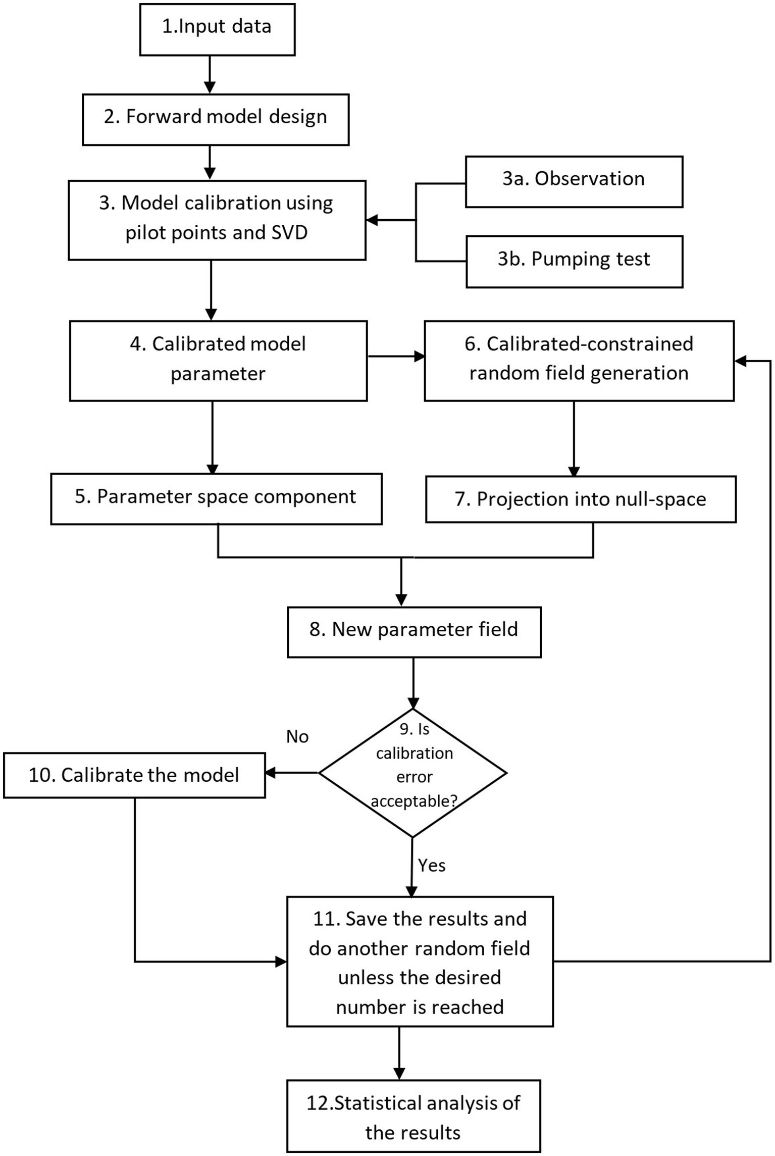
Figure 2. Stepwise methodology of the NSMC.

Figure 3

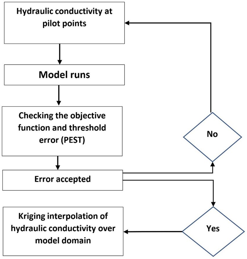
Figure 3. Calibration stepwise methodology used in box 3 of Figure 2.

Figure 4

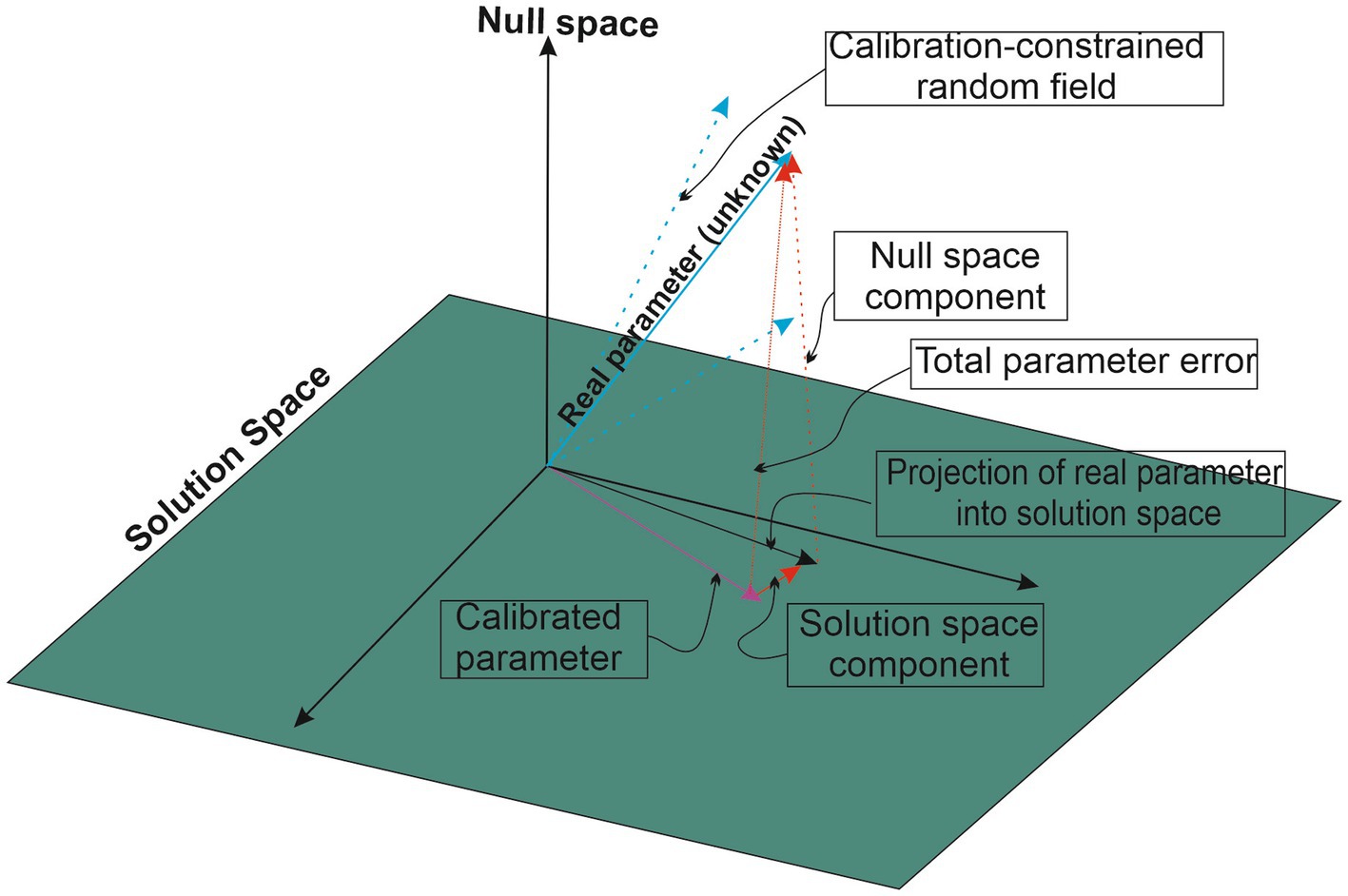
Figure 4. Null-Space Monte Carlo.

Running NSMC, as described above, was done using PEST code coupled with MODFLOW (Doherty, 2015). The calibrated parameter field, which is the hydraulic conductivity, is generated at the pilot point location, and the model is run. The model results are then checked against the field measurements to check the calibration error. If the error is accepted, then the values of hydraulic conductivity are interpolated over the model domain using kriging; otherwise, a new field is generated and the model is run again. It is important to note that the calibration results involve solving an inverse problem, which is inherently ill-posed. As such, the solution is non-unique, implying that there could be various configurations of hydraulic conductivity distributions that effectively calibrate the model.

3.2 Model description

The model domain was discretized into a 500 × 500-m finite difference grid, covering the north aquifer presented in Figure 1. The model domain is bounded by the sea to east, north, and west directions, and these are considered constant-head boundaries. No flow occurs at the southern boundary of the aquifer as both aquifers are hydraulically disconnected (Eccleston et al., 1981). The USGS finite difference-based MODFLOW-2005 model was used to simulate steady-state conditions of the groundwater flow (Harbaugh, 2005). The hydraulic conductivity field statistics are initially established using literature values and aquifer test data (Eccleston et al., 1981; Schlumberger Water Services, 2009; Baalousha, 2016b). Schlumberger Water Services (2009) conducted 11 pumping tests in the northern aquifer. In addition, Eccleston et al. (1981) have done many other tests in the past in the entire country. These results are used in the calibration process. The minimum, maximum, and average values of transmissivity are 20, 1,320, and 305 m²/d, respectively.

The calibration targets are the groundwater heads at 38 observation wells (Figure 1). These data refer to the year 1958 when the aquifer status was steady and the pumping rate was negligible (Eccleston et al., 1981). Rainfall recharge was based on the long-term average, representing natural conditions before development (Baalousha, 2016a). A total of 38 bores were found in the north aquifer, as depicted in Figure 1.

The calibrated parameter is the hydraulic conductivity. The NSMC is employed to produce multiple realizations of hydraulic conductivity (K) fields while adhering to the constraints of the calibration. Consequently, all resulting realizations contribute to a well-calibrated model. The variability present in these K-fields reflects the inherent uncertainty in our understanding of the system and its representation within the model.

4 Results

4.1 Calibrated model results

The initial step in the NSMC involves obtaining calibrated model results through the utilization of pilot points and kriging spatial interpolation. This is important as the kriging variogram properties are employed in the NSMC within the PEST code (Doherty, 2015). Figure 5 displays the calibrated model results for the study area, depicting variations in the head from near-zero levels along the shoreline to 18 m above the mean sea level (m. s. l.) further inland. Calibration statistics, presented in Table 1, revealed a mean weighted residual for both flow mass balance and head, along with a root mean square error of 0.7 for hydraulic conductivity. In addition, the mean residual of the head was −0.03 m, whereas the mean residual of flow was 0. These values are reliable indicators of the goodness of the calibration process.

Figure 5

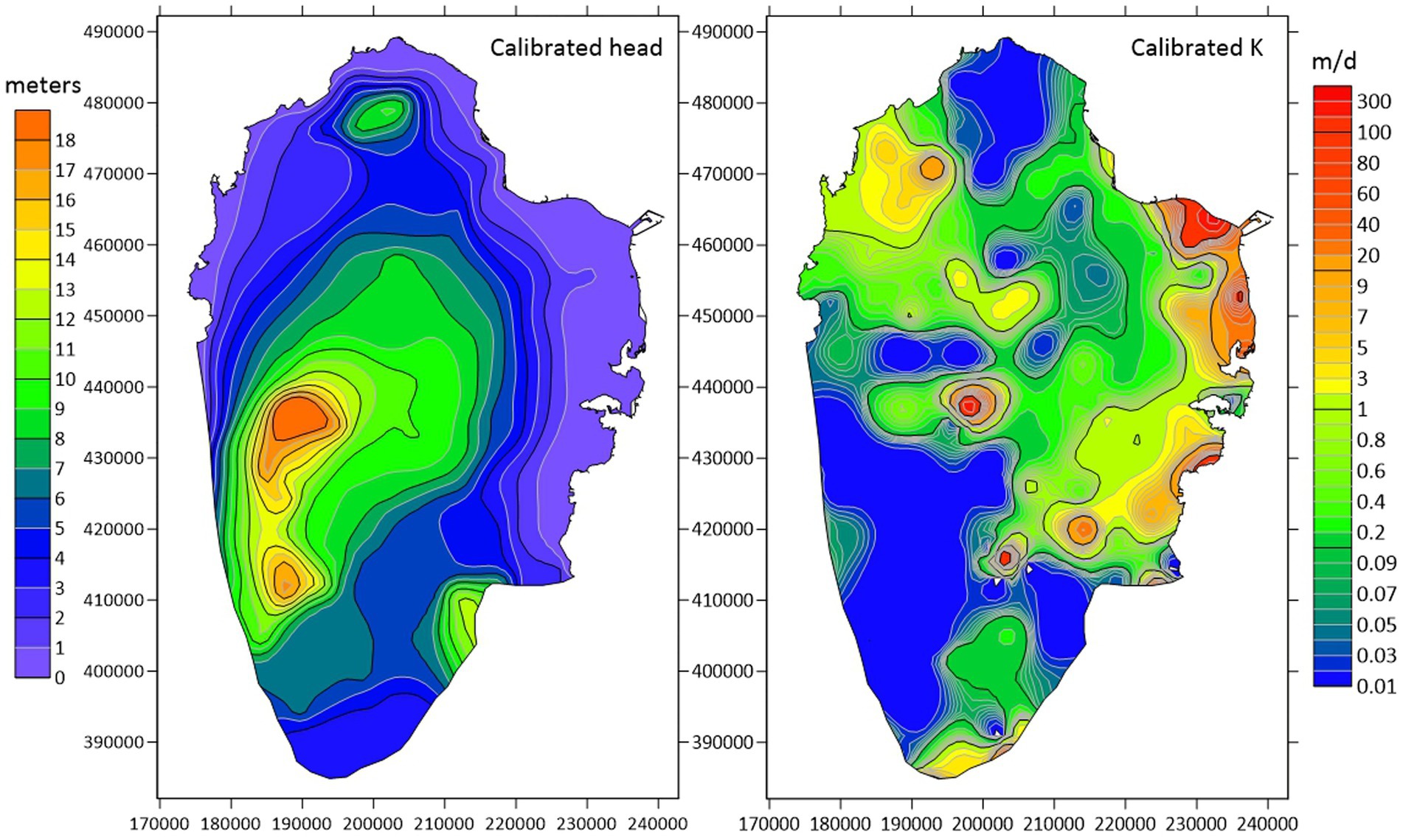
Figure 5. Left: steady-state calibrated head (meters a.m.s.l.), and right: calibrated hydraulic conductivity.

Table 1

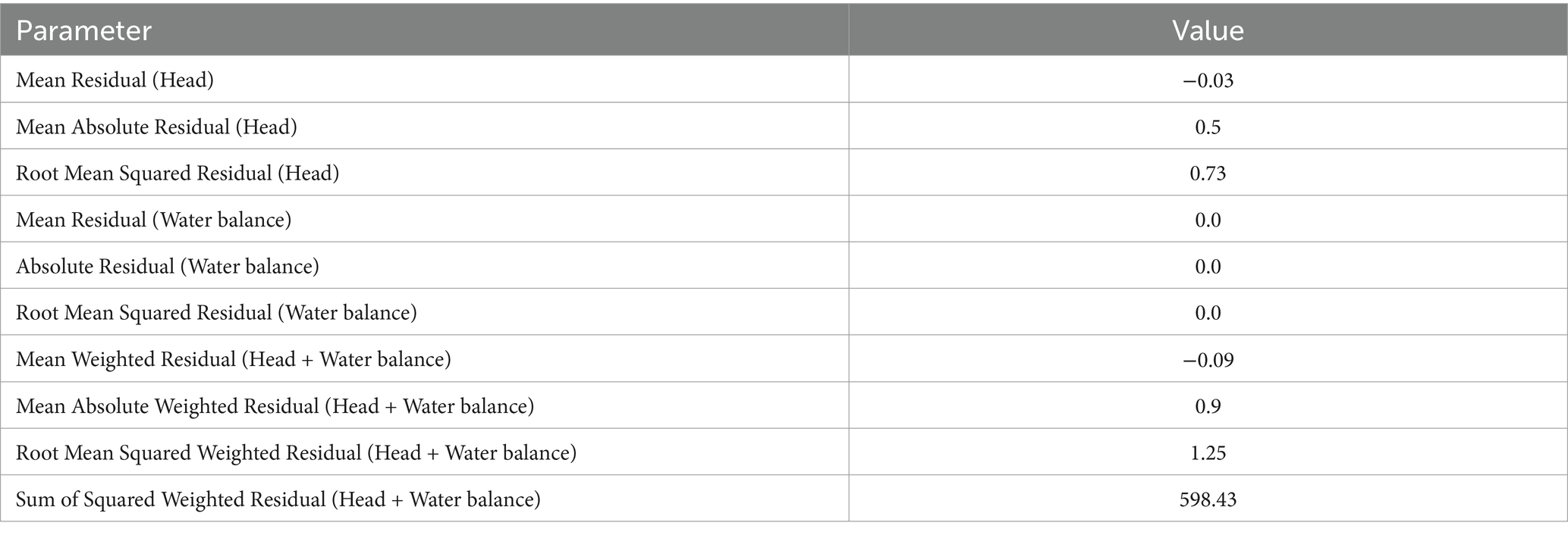
Table 1. Statistics of calibration.

The calibrated values of hydraulic conductivity range from 0.01 to more than 300 m/d, as depicted in Figure 5 (right). This considerable variation was indicative of the inherent heterogeneity of the karst aquifer. The results further reveal that higher hydraulic conductivity values were concentrated near the shoreline in the east-north region and inland in the central to southern parts of the aquifer.

4.2 Null-space Monte Carlo results

As discussed in the methodology, 200 calibration-constrained Monte Carlo realizations were generated, and in each run, the hydraulic conductivity field was checked against the calibrated values. The results showed that in all 200 runs, there was a need to recalibrate the model, owing to its high non-linearity. In some cases, the number of runs required to reach an acceptable solution was higher than that needed to calibrate the model in the first step. Figure 6 depicts the statistics of the NSMC runs. The mean hydraulic head varied between 0 and 17 m (m. s. l.), with a standard deviation that varied between 0 and 4 m (m. s. l.). It is noted that the high standard deviations occur in the middle of the study area, where the hydraulic head is high. The minimum and maximum hydraulic head values vary between 0–12 m and 0–21 m (a. m. s. l.), respectively.

Figure 6

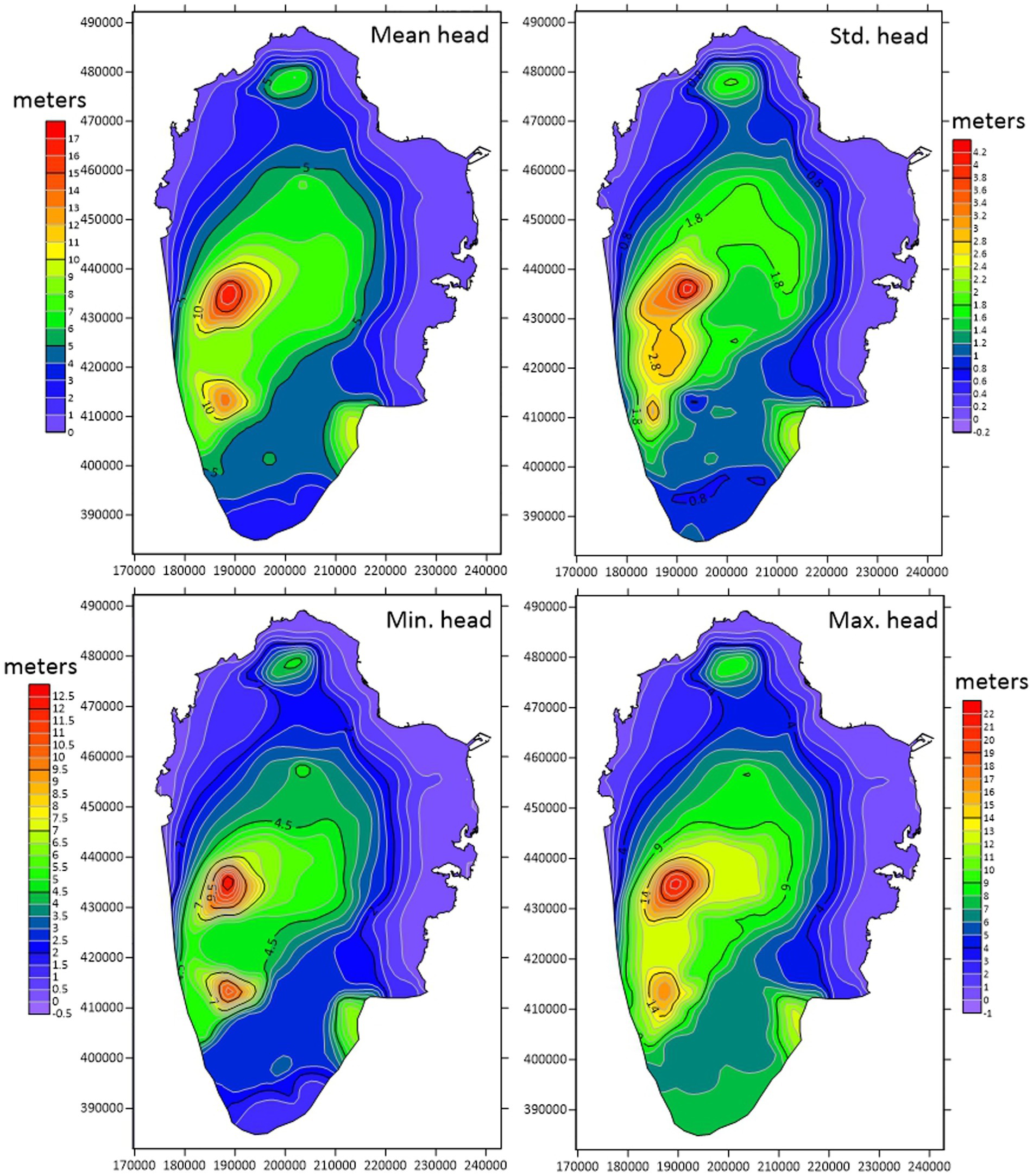
Figure 6. Statistical analysis of head resulting from 200 NSMC runs.

Figure 7 shows the statistics of hydraulic conductivity values obtained through NSMC, including the mean, standard deviation, minimum, and maximum. The mean hydraulic conductivity showed significant variability, ranging from 2.5E-4 to 331 m/d, indicating a distinct heterogeneity. The distribution of mean hydraulic conductivity, derived from 200 runs, closely aligned with that obtained from the calibrated model (Figure 7 right). Notably, the highest values were observed in the southern part of the aquifer, and a smaller region in the north-east was characterized by the outcropping of the Rus Formation and the occurrence of many fractures (Figure 1). Pumping test data reported by Schlumberger Water Services (2009) and Eccleston et al. (1981) revealed high transmissivity in this area, which is confirmed by this study. The standard deviation varied from 7.6E-06 to 173 m/d, with the highest values corresponding to the areas with elevated mean conductivity.

Figure 7

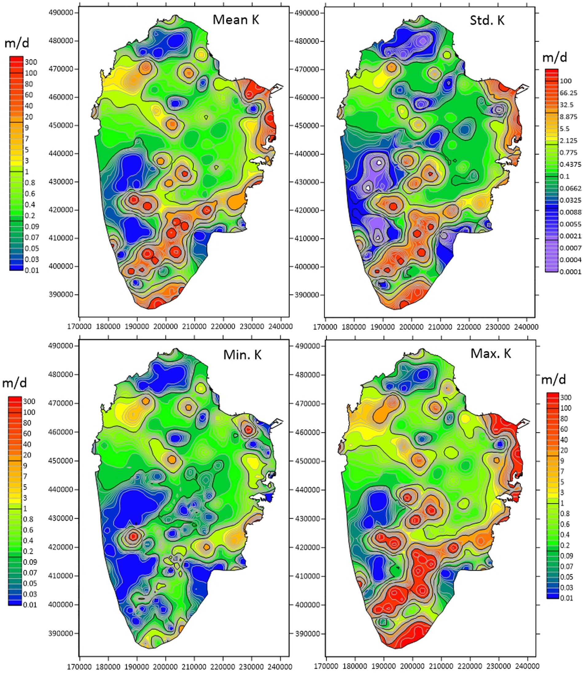
Figure 7. Statistical analysis of hydraulic conductivity (m/d) resulting from 200 NSMC runs.

The minimum values of hydraulic conductivity vary between 1.1E-3 and 295.3 m/d, while the maximum values span from 8.2E-5 to 350 m/d. The distribution of maximum values closely resembles that of the mean value, whereas the distribution of minimum values shows a different pattern. Table 2 presents the descriptive statistics for both mean head and mean hydraulic conductivity. While the mean value of the head shows a slight deviation from the median, this deviation is more pronounced in the case of hydraulic conductivity. The mean value of hydraulic conductivity is 16.783 m/d, whereas the median is 0.859 m/d. On the other hand, the mean value of the mean head is 5.5 m, and the median is 5.2 m. This slight discrepancy between the mean and the median suggests a more or less normal distribution of head values. The distribution of hydraulic conductivity exhibits a clear rightward skewness, indicating that the majority of the aquifer has lower hydraulic conductivity. Statistical analysis reveals that only 10 of the aquifer cells have hydraulic conductivity higher than 50 m/d. Altogether, the descriptive statistics collectively indicate a high degree of heterogeneity.

Table 2

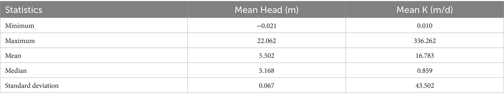
Table 2. Descriptive statistics of mean head and mean hydraulic conductivity.

5 Conclusion

The inverse problem is highly challenging for modelers, given its non-unique solution. Addressing this problem usually requires a high computational cost due to the high number of iterations required. Techniques such as crude Monte Carlo simulations demand a high number of iterations to achieve an acceptable level of accuracy, primarily due to their slow convergence rate. Utilizing these methods for uncertainty analysis increases the computation requirements further. Given the non-uniqueness of the inverse problem solution, it is important to evaluate the uncertainty associated with the resulting calibrated parameter field. The study explores the application of the NSMC method for uncertainty analysis in the model calibration of a highly parameterized karst carbonate aquifer in Qatar. The NSMC method, a constrained Monte Carlo approach, makes use of the null-space component of a randomly generated vector of calibrated parameters. The results have important implications for groundwater management in karst carbonate aquifers. The uncertainty of hydraulic conductivity is important because it directly affects the reliability of groundwater flow models, resource management decisions, and environmental protection measures. Uncertainty in hydraulic conductivity affects the estimation of groundwater availability and sustainability. It can also affect the transport of contaminants, solutes, and other substances in groundwater. High uncertainty in hydraulic conductivity can lead to unreliable groundwater flow predictions, affecting decision-making. By quantifying uncertainty, stakeholders can make more informed decisions and effectively manage groundwater systems for the benefit of society and the environment.

Uncertainty analysis of the calibrated field of the karst aquifer under consideration reveals that high uncertainty aligns with areas of high hydraulic conductivity. Although the variation in hydraulic conductivity between the minimum and maximum values is not high, the absolute measure of variability, as indicated by the standard deviation, is notably high, particularly in regions of high hydraulic conductivity uncertainty.

To apply NSMC, the model must undergo calibration initially, leading to the obtaining of geostatistics for the calibrated parameters. The calibrated parameter was then decomposed into a null space and a solution space. The latter was combined with a null space resulting from a randomly generated vector. The results indicate that while the NSMC produces diverse fields of hydraulic conductivity, all of which successfully calibrate the model, numerous iterations are required to reach a solution within the specified error threshold. This contrasts with the suggestions in the literature (Doherty, 2015) and is likely attributed to the high heterogeneity of the aquifer modeled in this study, introducing a highly non-linear solution. As such, the use of NSMC provides little advantage over other uncertainty methods in the case of high non-linearity, such as karst aquifers with high variability.

Data availability statement

The original contributions presented in the study are included in the article/supplementary material, further inquiries can be directed to the corresponding author.

Author contributions

HB: Conceptualization, Data curation, Formal analysis, Funding acquisition, Investigation, Methodology, Project administration, Resources, Software, Supervision, Validation, Visualization, Writing – original draft, Writing – review & editing.

Funding

The author(s) declare that no financial support was received for the research, authorship, and/or publication of this article.

Acknowledgments

The author would like to thank King Fahd University of Petroleum and Minerals (KFUPM) for supporting this research.

Conflict of interest

The author declares that the research was conducted in the absence of any commercial or financial relationships that could be construed as a potential conflict of interest.

The handling editor MF declared a shared affiliation with the author HB at the time of review.

Publisher’s note

All claims expressed in this article are solely those of the authors and do not necessarily represent those of their affiliated organizations, or those of the publisher, the editors and the reviewers. Any product that may be evaluated in this article, or claim that may be made by its manufacturer, is not guaranteed or endorsed by the publisher.

References

Al-Hajari, S. (1990). Geology of the tertiary and its influence on the aquifer system of Qatar and eastern Arabia. Ph.D. thesis. Carolina: University of South Carolina.

Google Scholar

Alsharhan, A., Rizk, Z., Nairn, A., Bakhit, D., and Alhajari, S. (2001). Hydrogeology of an arid region: The Arabian gulf and adjoining areas. Amsterdam: Elsevier Science B.V.

Google Scholar

Amini, M., Abbaspour, K. C., Berg, M., Winkel, L., Hug, S. J., Hoehn, E., et al. (2008). Statistical modeling of global Geogenic arsenic contamination in groundwater. Environ. Sci. Technol. 42, 3669–3675. doi: 10.1021/es702859e

PubMed Abstract | Crossref Full Text | Google Scholar

Baalousha, H. (2006). Groundwater pollution risk using a modified Latin hypercube sampling. J. Hydroinf. 8, 223–234. doi: 10.2166/hydro.2006.018b

Crossref Full Text | Google Scholar

Baalousha, H. (2009). Stochastic water balance model for rainfall recharge quantification in Ruataniwha Basin, New Zealand. Environ. Geol. 58, 85–93. doi: 10.1007/s00254-008-1495-6

Crossref Full Text | Google Scholar

Baalousha, H. M. (2016a). Development of a groundwater flow model for the highly parameterized Qatar aquifers. Model. Earth Syst. Environ. 2:67. doi: 10.1007/s40808-016-0124-8

Crossref Full Text | Google Scholar

Baalousha, H. M. (2016b). The potential of using beach wells for reverse osmosis desalination in Qatar. Model. Earth Syst. Environ. 2:97. doi: 10.1007/s40808-016-0151-5

Crossref Full Text | Google Scholar

Baalousha, H., Fahs, M., Ramasomanana, F., and Younes, A. (2019). Effect of pilot-points location on model calibration: application to the northern karst aquifer of Qatar. Water 11:679. doi: 10.3390/w11040679

Crossref Full Text | Google Scholar

Baalousha, H. M., Ramasomanana, F., Fahs, M., and Seers, T. D. (2022). Measuring and validating the actual evaporation and soil moisture dynamic in arid regions under unirrigated land using smart field Lysimeters and numerical modeling. Water 14:2787. doi: 10.3390/w14182787

Crossref Full Text | Google Scholar

Baalousha, H. M., Tawabini, B., and Seers, T. D. (2021). Fuzzy or non-fuzzy? A comparison between fuzzy logic-based vulnerability mapping and DRASTIC approach using a numerical model. A case study from Qatar. Water 13:1288. doi: 10.3390/w13091288

Crossref Full Text | Google Scholar

Baalousha, H. M., Younes, A., Yassin, M. A., and Fahs, M. (2023). Comparison of the fuzzy analytic hierarchy process (F-AHP) and fuzzy logic for flood exposure risk assessment in arid regions. Hydrology 10:136. doi: 10.3390/hydrology10070136

Crossref Full Text | Google Scholar

Beven, K., and Binley, A. (1992). The future of distributed models: model calibration and uncertainty prediction. Hydrol. Process. 6, 279–298. doi: 10.1002/hyp.3360060305

Crossref Full Text | Google Scholar

Carrera, J., Alcolea, A., Medina, A., Hidalgo, J., and Slooten, L. J. (2005). Inverse problem in hydrogeology. Hydrogeol. J. 13, 206–222. doi: 10.1007/s10040-004-0404-7

Crossref Full Text | Google Scholar

Doherty, J. (2015). Calibration and uncertainty analysis for complex environmental models. Australia: Watermark Numerical Computing.

Google Scholar

Doherty, J. E., Fienen, M. N., and Hunt, R. J. (2011). Scientific investigations report. scientific investigations report. Series Scientific Investigations Report

Google Scholar

Eccleston, B. L., Pike, J., and Harhash, I. (1981). The water resources of Qatar and their development: Vol I. Tech. Rep. Vol I, food and agricultural Organization of the United Nations, Doha, Qatar.

Google Scholar

Formentin, G., Terrenghi, J., Vitiello, M., and Francioli, A. (2019). Evaluation of the performance of a hydraulic barrier by the null space Monte Carlo method. Acque Sotterranee Ital. J. Groundw. 2019:420. doi: 10.7343/as-2019-420

Crossref Full Text | Google Scholar

Harbaugh, A. W. (2005). MODFLOW-2005, the U.S. Geological Survey modular ground-water model–the ground-water flow process: U.S. Geological Survey Techniques and Methods 6-A16, variously.

Google Scholar

Hardyanto, W., and Merkel, B. (2007). Introducing probability and uncertainty in groundwater modeling with FEMWATER-LHS. J. Hydrol. 332, 206–213. doi: 10.1016/j.jhydrol.2006.06.035

Crossref Full Text | Google Scholar

Harvey, C. F., and Gorelick, S. M. (1995). Temporal moment-generating equations: modeling transport and mass transfer in heterogeneous aquifers. Water Resour. Res. 31, 1895–1911. doi: 10.1029/95WR01231

Crossref Full Text | Google Scholar

Hassan, A. E., Bekhit, H. M., and Chapman, J. B. (2009). Using Markov chain Monte Carlo to quantify parameter uncertainty and its effect on predictions of a groundwater flow model. Environ. Model Softw. 24, 749–763. doi: 10.1016/j.envsoft.2008.11.002

Crossref Full Text | Google Scholar

Iman, R. L., Campbell, J. H., and Helton, J. C. (1981). An approach to sensitivity analysis of computer models: part I—introduction, input variable selection and preliminary variable assessment. J. Qual. Technol. 13, 174–183. doi: 10.1080/00224065.1981.11978748

Crossref Full Text | Google Scholar

Jacob, D., Ackerer, P., Baalousha, H. M., and Delay, F. (2021). Large-scale water storage in aquifers: enhancing Qatar’s groundwater resources. Water 13:2405. doi: 10.3390/w13172405

Crossref Full Text | Google Scholar

Kimrey, J. O. (1985). Proposed artificial recharge studies in northern Qatar. Report, 85–343. doi: 10.3133/ofr85343

Crossref Full Text | Google Scholar

Mckay, M. D., Beckman, R. J., and Conover, W. J. (1979). A comparison of three methods for selecting values of input variables in the analysis of output from a computer code. Technometrics 21:239. doi: 10.2307/1268522

Crossref Full Text | Google Scholar

Moeck, C., Molson, J., and Schirmer, M. (2020). Pathline density distributions in a null-space Monte Carlo approach to assess groundwater.Pdf. Ground Water 58, 189–207. doi: 10.1111/gwat.12900

Crossref Full Text | Google Scholar

Owen, A. B. (1992). A central limit theorem for Latin hypercube sampling. J. R. Stat. Soc. Ser. B (Methodological) 54, 541–551. doi: 10.1111/j.2517-6161.1992.tb01895.x

Crossref Full Text | Google Scholar

RamaRao, B. S., LaVenue, A. M., De Marsily, G., and Marietta, M. G. (1995). Pilot point methodology for automated calibration of an ensemble of conditionally simulated transmissivity fields: 1. Theory and computational experiments. Water Resour. Res. 31, 475–493. doi: 10.1029/94WR02258

Crossref Full Text | Google Scholar

Ren, L., He, L., Lu, H., and Chen, Y. (2016). Monte Carlo-based interval transformation analysis for multi-criteria decision analysis of groundwater management strategies under uncertain naphthalene concentrations and health risks. J. Hydrol. 539, 468–477. doi: 10.1016/j.jhydrol.2016.05.063

Crossref Full Text | Google Scholar

Schlumberger Water Services . (2009). Studying and developing the natural and artificial recharge of the groundwater aquifer in the state of Qatar-final project report. Technical Report, Doha, Qatar.

Google Scholar

Sepulveda, N., and Doherty, J. (2015). Uncertainty analysis of a groundwater flow model in east-central´ Florida. Groundwater 53, 464–474. doi: 10.1111/gwat.12232

Crossref Full Text | Google Scholar

Tonkin, M., and Doherty, J. (2009). Calibration-constrained Monte Carlo analysis of highly parameterized models using subspace techniques. Water Resour. Res. 45:6678. doi: 10.1029/2007WR006678

Crossref Full Text | Google Scholar

Tziatzios, G., Sidiropoulos, P., Vasiliades, L., Lyra, A., Mylopoulos, N., and Loukas, A. (2021). The use of the pilot points method on groundwater modelling for a degraded aquifer with limited field data: the case of Lake Karla aquifer. Water Supply 21, 2633–2645. doi: 10.2166/ws.2021.133

Crossref Full Text | Google Scholar

Vecchioli, J. (1976). Preliminary evaluation of the feasibility of artificial recharge in northern Qater. Report, 76–540. doi: 10.3133/ofr76540

Crossref Full Text | Google Scholar

Wu, J., and Zeng, X. (2013). Review of the uncertainty analysis of groundwater numerical simulation. Chin. Sci. Bull. 58, 3044–3052. doi: 10.1007/s11434-013-5950-8

Crossref Full Text | Google Scholar