Comparison of two hydrodynamic models for their rain-on-grid technique to simulate flash floods in steep catchment

In this study, two hydrodynamic models, TELEMAC-2D and HEC-RAS 2D, were compared for their Rain-on-Grid (RoG) technique with a particular focus on runoff generation processes in a small and steep catchment. Curve number (CN) method was applied in both the models to simulate two single storm events up to 20 h of duration, whereas the Green-Ampt Redistribution (GAR) method was additionally applied in HEC-RAS 2D for a multi-peak flood event with sustained flow between the peaks. CN and GAR methods were compared for this flood event, and a sensitivity analysis of the GAR parameters was also done. Moreover, the two models were compared for their calibration process, computational time, mesh size and shape, and model availability, in general, as well as the results including inundated areas, water depth, and velocity. The results indicate that both the models are capable of reproducing short duration single storm floods. NSE and R² for both models ranged from 0.70 to 0.90 and from 0.93 to 0.95. However, the models struggled to reproduce the long- duration multi-peak flood event. The sensitivity analysis showed that the results are not very sensitive to the two GAR parameters which are responsible to influence the flow of the second peak in the flood event. Neither the CN nor the GAR infiltration method successfully replicated such events because the hydraulic models permanently lose infiltrated water from the domain. The returned sub-surface flow significantly contributes to river flow during these flood events; however, none of the model incorporates a return flow algorithm.

1 Introduction

Frequency of extreme rainfall events has been increasing in recent years leading to extreme floods. The frequency and magnitude of such events are likely to increase in the future because of global warming and changing climate (Seneviratne et al., 2021), urbanization, land use, and infrastructure development (Feng et al., 2021). When there is a sudden, violent rise in water level and high peak flows within less than 6 h, it is referred as a flash flood (Sweeney, 1992; Marchi et al., 2010; Kishore and Rishi, 2014; Zhang et al., 2019). Floods of this nature can occur due to factors such as extreme precipitation and temperatures, rain-on-snow events, snowmelt, glacial lake outbursts (Jha and Khare, 2016), volcanic eruptions (Basso-Báez et al., 2020), or dam breaks.

The adverse environmental impacts of flash floods can include soil erosion, riverbank and bed erosion (Swanston, 1974), and debris flow (Borga et al., 2014) and may lead to sedimentation and river overflow (Johnson et al., 2010) and even landslides (Lin et al., 2021). Floodwater can also harm vegetation, whereas pollutants transported by it may adversely affect water quality, habitats, and flora and fauna. A case study by Vázquez Conde et al. (2001) describes that huge amount of fine and coarse sediments was transported by flash flood in Mexico. These sediments not only reduced the discharge capacity of the river but also contributed to the rise of the water level and eventually killed more than 800 people. Flash floods have been one of the most damaging natural hazards throughout the world (Maatar et al., 2015) in terms of loss of lives, property, and environmental damage (Liu et al., 2022). Furthermore, flash floods have contributed to 40% of the total casualties in Europe from 1950 to 2006 (Barredo, 2007). Thus, it is crucial to analyze flash flood events and the consequences in an efficient way using the hydrologic and hydraulic characteristics of such events.

Flash floods in small and steep mountainous catchments can be particularly dangerous as they lead to a rapid rise in discharge and water velocities (Bruland, 2020; Moraru et al., 2021). Complex topography and meteorological complexity in such catchments make it even more difficult to model flash floods (Li et al., 2020; Maqtan et al., 2022). Usually, flood scenarios are modeled using hydrological and hydraulic models separately. Hydrological models are used to calculate the discharge (hydrograph) at a point in the catchment, whereas the hydrodynamic models are used to simulate the hydraulic characteristics with given inflows to the water course. Such characteristics include flow velocity, water depth, submerged area, shear stress, erosion, and sedimentation. An output hydrograph from a hydrological model or an observed hydrograph is usually used as input or boundary condition to the hydrodynamic model. The two types of models can be integrated manually, but that is a laborious process due to the need for separate calibration and running simulations in the two models. Additionally, both establishing the boundary conditions and determining their placement along the water course in the hydrodynamic model can be challenging. Thus, the boundary condition is usually not set for small tributaries, resulting in inaccurate discharge predictions along the main river. Hence, to address these issues, this study has used a Rain-on-Grid technique implementation in hydrodynamic models (HDRRM- Hydrodynamic Rainfall-Runoff Models). This technique defines the river network in the catchment and provides the inflow to any point along the rivers and streams.

The Rain-on-Grid (RoG) technique or the direct rainfall method (DRM) is a method in which precipitation is used directly as input over the grid cells in a hydrodynamic model. This method integrates both hydrological and hydrodynamic calculations within a single model, eliminating the need for manual integration of the two model types. Thus, in contrast to traditional 1D/2D hydraulic modeling, the inflow to the water courses is fed continuously along the rivers and the tributaries rather than through defined boundaries. Even though hydrodynamic routing between all grid cells across the entire catchment is computationally more demanding than restricting it to grid cells within the water course, it was observed to be more efficient compared with the offline coupling of the two model types (Rangari et al., 2019; David and Schmalz, 2021; Zeiger and Hubbart, 2021).

In this study, we compare the performance of two hydrodynamic models, TELEMAC-2D (Ligier, 2016) and HEC-RAS 2D (Brunner, 2002) for their Rain-on-Grid (RoG) technique in a steep catchment to find out their limitations and strengths. RoG implementation in TELEMAC-2D (T2D hereafter) has been tested before to model flash floods in a steep and small snow-covered catchment (Godara et al., 2023b), and it was found that the model was able to reproduce single storm flood events but struggled to reproduce all peaks in a sustained flow event with multiple peaks. Therefore, the first objective of this study is to check if HEC-RAS 2D (HR2D hereafter) can achieve equally good results as T2D for simulating single storm flood events. The second objective of this comparison is to check if HR2D is able to reproduce long duration of flood events better than T2D. A particular focus for the second objective has been on how they handle the hydrology, i.e., infiltration and generation of rainfall excess and the long duration of multi-storm events. T2D uses the Curve-Number (CN) method to determine the infiltration rate and the remaining portion of the rainfall from each cell goes to runoff (Ligier, 2016). HEC-RAS 2D (HR2D hereafter) has three optional methods for calculating the infiltration: Deficit and Constant Loss method, CN method, and Green-Ampt Redistribution (GAR) method (Brunner, 2020), where CN and GAR are the two methods used in this study. Moreover, the two models are compared for their calibration process, computational time, mesh size and shape, and model availability, in general, as well as the inundated areas, water depths, and velocity of water after a rainfall event. The current study is one of the first to compare these two hydrodynamic models for their rain-on-grid rainfall-runoff modeling.

2 Materials and methods

2.1 Study area and input data

The Sleddalen catchment in Møre og Romsdal county in western Norway was selected for this study. This catchment is selected because it is steep and has the potential of disastrous flash floods and a discharge measurement station. It is a steep mountainous catchment with an area of 10.5 km² and average slope of 0.5 m/m with highest and lowest elevations at 1,379 and 77 m, respectively. The catchment is mostly covered by open land, forest, bare rock, and scarce vegetation, as shown in Figure 1 (generated using QGIS version 3.34).

Figure 1

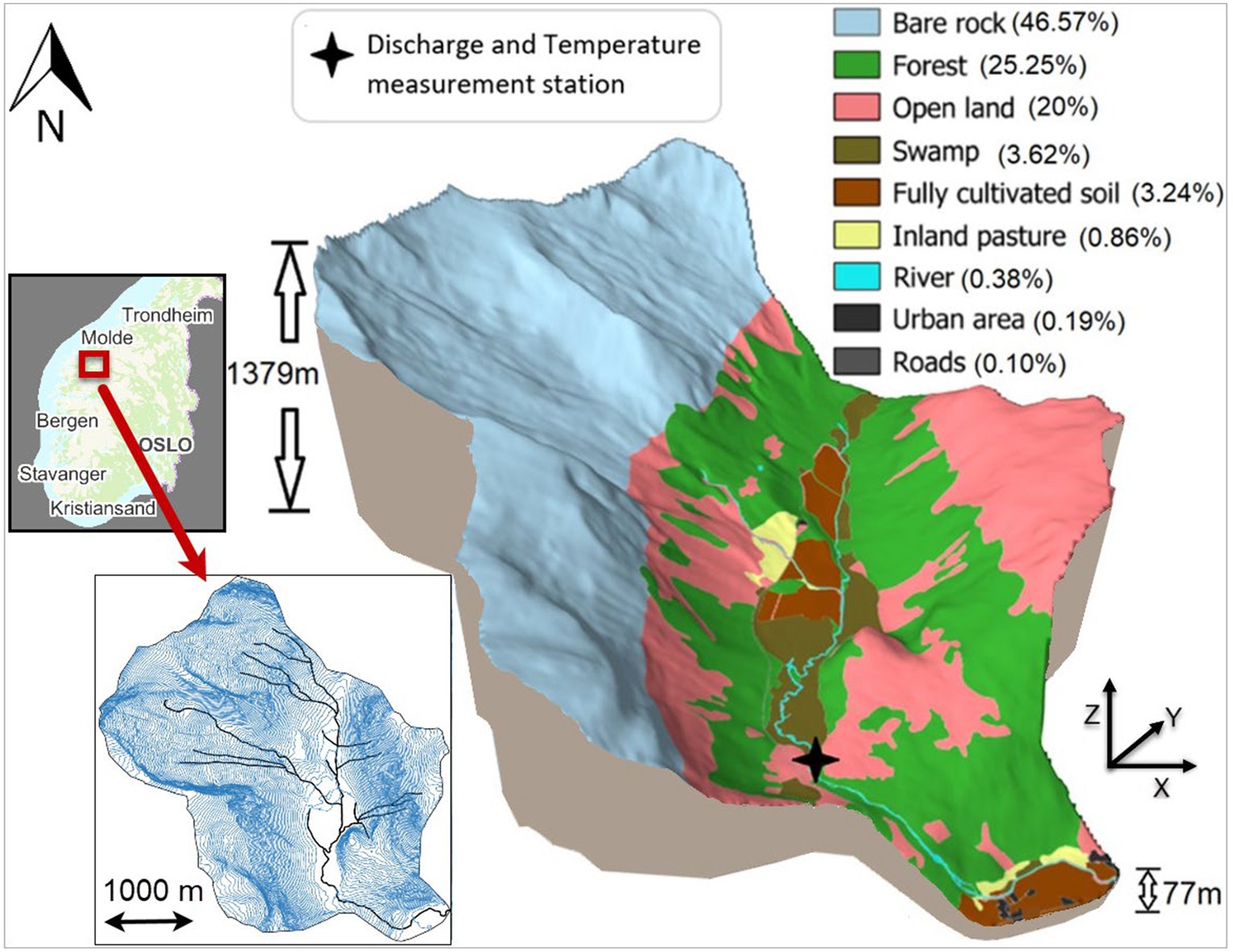
Figure 1. Study area showing steepness and land cover-land use information with the percentage of each type, maximum and minimum elevation levels in the catchment, and the location of discharge and temperature measurement stations. Small figure in bottom left shows the DTM of the area with contour lines at 10 m vertical distance along with a digitized river network from the Norwegian Water Administration database.

The input data used for this study are digital terrain model (DTM), observed discharge, and temperature and precipitation data. DTM data with a resolution of 0.5 m by 0.5 m were downloaded from the Norwegian mapping authority database.¹ The observed discharge data with 15 min of resolution and temperature data with 1 h of resolution were taken from the measurement station (Sleddalen station ID: 97.5.0) inside the catchment, as shown in Figure 1. Precipitation data with 1 km by 1 km spatially distribution and 1 h temporal resolution were extracted from the RadPro dataset which is a merged product of gridded precipitation point observations and precipitation radar data (Engeland et al., 2018). Land use–land cover data were downloaded from Geonorge² which is a Norwegian national website for maps and other geographical information in Norway. Two high flow events up to 20 h of duration induced by single storm rainfall events and one longer duration event with sustained flow between the storms induced by a multi-storm rain-on-snow event were selected for this study.

2.2 Models and methods

2.2.1 Model concepts, availability, installation, and input file preparation

In this study, two hydraulic models, T2D and HR2D, are used for the hydrodynamic rainfall-runoff modeling (HDRRM). These models have an option to use the precipitation data directly as input to the model grid cells also called the rain-on-grid (RoG) technique (David and Schmalz, 2021). Both the models are based on solving the Shallow Water Equations (SWE), which are derived from the Navier–Stokes equations. T2D is a freely available and open-source model. The users can change and implement new methods themselves in the source code of this model. On the other hand, HR2D is freely available but not open source. RoG was recently introduced in HR2D (Zeiger and Hubbart, 2021; Hariri et al., 2022) and it has a graphical user interface (GUI) which makes its use and installation easier than T2D. For the same reason, preparation of the input files is also less time-consuming for HR2D. RAS-mapper alone was used for pre- and post-processing and visualization of the results, whereas in T2D, various software and programs such as Bluekenue, QGIS, R, and Python were used.

2.2.2 TELEMAC-2D

T2D calculates water depth and the components of velocity in two dimensions of horizontal space using a computational mesh of triangular elements (Figure 2). Various numerical methods are available in T2D for solving shallow water equations such as the finite-volume and finite-element method (Sarker, 2022), but finite-volume is utilized in this study. T2D can work on up to eight parallel core processers in a CPU computer. T2D version v8p2 was used in this research study. Main input files required are the boundary condition file (*cli), precipitation file (*.slf), simulation file (CAS file), and geometry file (*.slf) containing information about watershed characteristics, grid cells, Manning’s roughness, and CN values. Python and R were used for preprocessing and converting the precipitation file from netCDF file into a SELAFIN (*.slf) file. Bluekenue (Barton, 2019) was used for preparing the other input files. PostTelemac plugin in QGIS (3.34) was used for visualization of T2D results, creating inundation maps. Mesh size varies from a maximum of 100 meter triangle edges in the drainage area to a refined grid down to 5 meter edge in the vicinity of the river network and 3 meter edge inside the river downstream of the measurement stations. Steep slope correction for CN values was applied in the T2D simulations considering the mountainous catchment. The code in T2D model simultaneously solves the following hydrodynamic equations:

(a) Continuity equation:

$\begin{array}{ll}\frac{\partial h}{\partial t}+u.\nabla \left(h\right)+hdiv\left(u\right)=S_h& (1)\end{array}$

(b) Momentum equation along x:

$\begin{array}{ll}\frac{\partial u}{\partial t}+u·\nabla \left(u\right)=-g\frac{\partial Z}{\partial x}+S_x+\frac{1}{h}div\left(h{v}_t\nabla u\right)& (2)\end{array}$

(c) Momentum equation along y:

$\begin{array}{ll}\frac{\partial v}{\partial t}+u·\nabla \left(v\right)=-g\frac{\partial Z}{\partial y}+S_y+\frac{1}{h}div\left(h{v}_t\nabla v\right)& (3)\end{array}$

where the equations are given here in Cartesian coordinates, and

$h$ (m) = water depth;

$u$, $v$ (m/s) = velocity components;

$g$ (m/s²) = gravity acceleration;

$v_t$ (m²/s) = momentum coefficient;

$Z$ (m) = free surface elevation;

$t$ (s) = time;

$x$, $y$ (m) = horizontal space coordinates;

$S_h$ (m/s) = source or sink of fluid; and

$h$, $u$, and $v$ are the unknowns

Figure 2

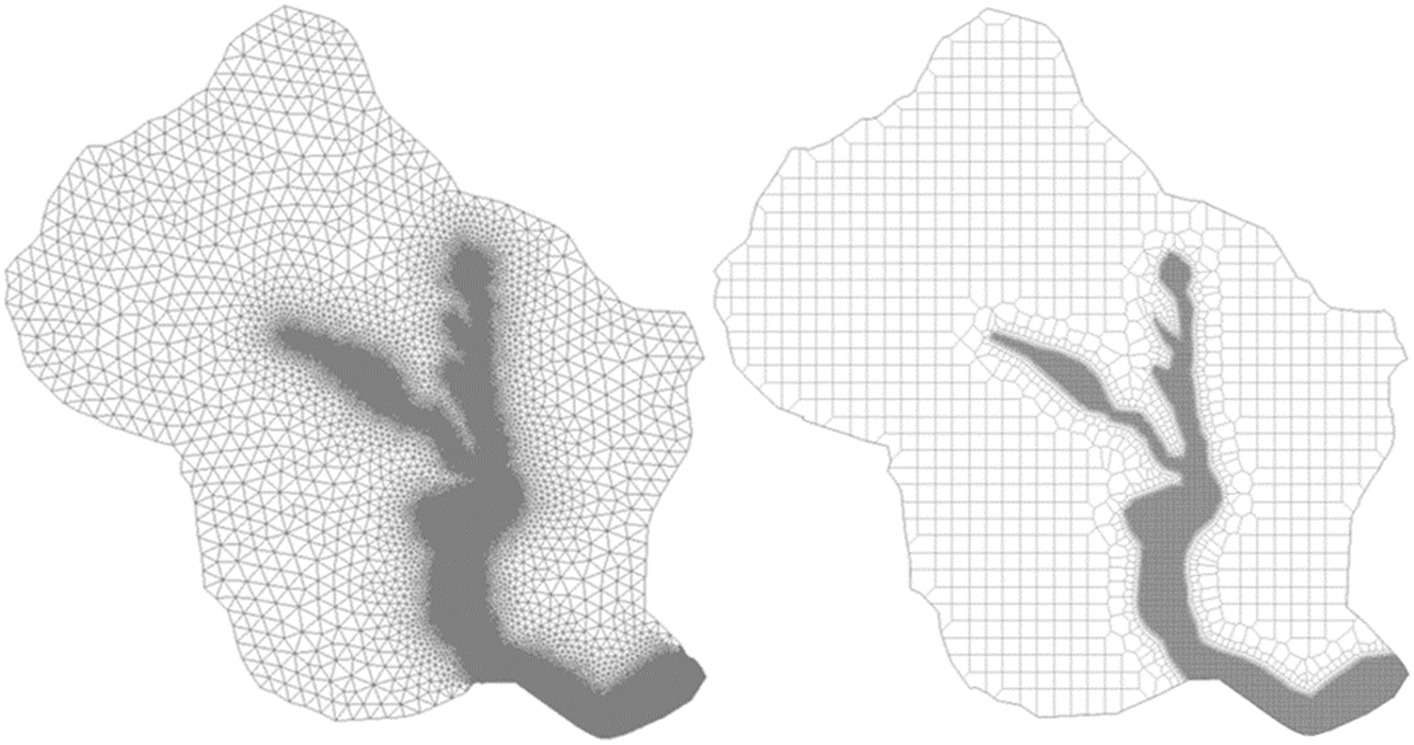
Figure 2. Triangle shaped mesh in T2D (104,566 cells) (left) and square shaped mesh in HR2D (56,106 cells) (right) with 5 m*5 m around and 3 m*3 m resolution in the river and 100 m*100 m resolution in rest of the catchment.

2.2.3 HEC-RAS 2D

The Hydrologic Engineering Center’s River Analysis System (HEC-RAS) version 6.3.1 was used in the current study. Input data required are similar to T2D except their formats. The precipitation file was used directly in netCDF format. Since HR2D has a user interface, the simulations can run directly from the main window of the HR2D unlike T2D. The model was run with the SWE-ELM (Eulerian–Lagrangian Method) equation set. HR2D uses a computational mesh of square shaped elements (Figure 2), and it allows for mesh refinement to increase the computational points to ensure numerical stability and increase the simulation precision in hydraulically complex regions. The initial mesh resolution used was similar to T2D (Figure 2), but later, the mesh was refined at various places by introducing more computational points (Figure 3B) due to the reasons explained in detail in the “Results” section. For both the models, Manning’s roughness and CN values were used in spatially distributed format (Table 1) based on the land cover types in the catchment (Figure 1).

Figure 3

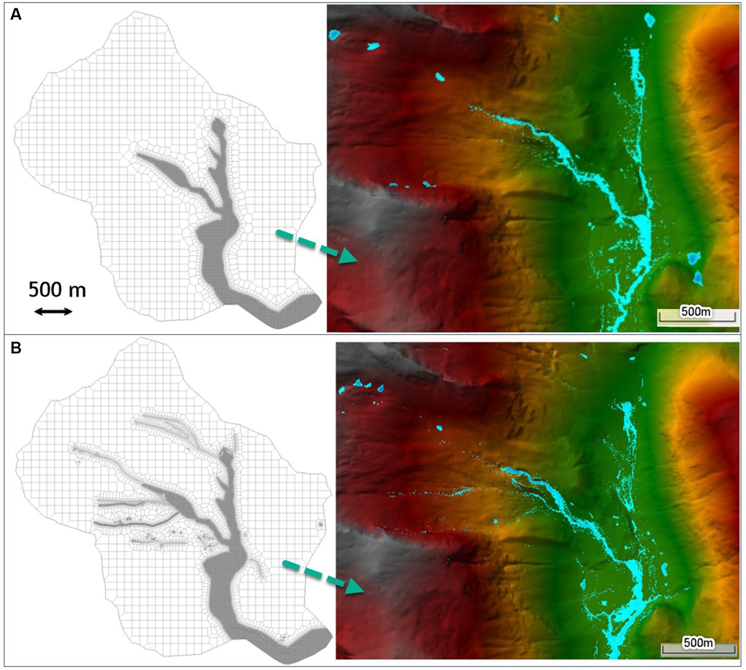
Figure 3. (A) Some of the artificial sinks where water was trapped at the end of the HR2D simulation for 100 m grid size, (B) Finer mesh breaklines to remove the artifact locations (approximately 56,000 cells).

Table 1

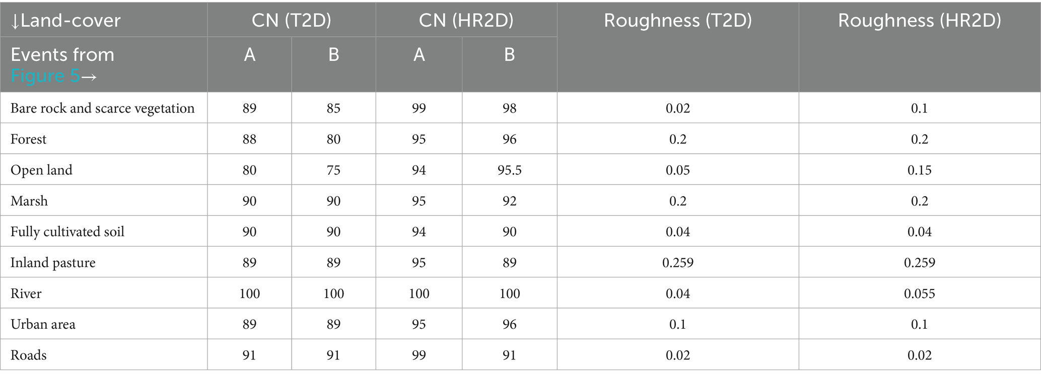
Table 1. Calibrated CN and Manning’s roughness values used for various land covers for both the models.

HR2D solves the following shallow water equations for its 2D modeling approach (Brunner, 2020):

(a) Continuity equation:

$\begin{array}{ll}\frac{\partial h}{\partial t}+\frac{\partial \left(hu\right)}{\partial x}+\frac{\partial \left(hv\right)}{\partial y}=q& (4)\end{array}$

(b) Momentum equations:

$\begin{array}{l}\frac{\partial u}{\partial t}+u\frac{\partial u}{\partial x}+v\frac{\partial u}{\partial y}-f_{c}v=-g\frac{\partial Z_S}{\partial x}+\frac{1}{h}\frac{\partial }{\partial x}\left(v_{t,xx}h\frac{\partial u}{\partial x}\right)\\ +\frac{1}{h}\frac{\partial }{\partial y}\left(v_{t,yy}h\frac{\partial u}{\partial y}\right)-\frac{{\tau }_{b,x}}{\rho R}+\frac{{\tau }_{s,x}}{\rho h}-\frac{1}{\rho }\frac{\partial p_a}{\partial x}\end{array}\text{ (5)}$

$\begin{array}{l}\frac{\partial v}{\partial t}+u\frac{\partial v}{\partial x}+v\frac{\partial v}{\partial y}-f_{c}u=-g\frac{\partial Z_S}{\partial y}+\frac{1}{h}\frac{\partial }{\partial x}\left(v_{t,xx}h\frac{\partial v}{\partial x}\right)\\ +\frac{1}{h}\frac{\partial }{\partial y}\left(v_{t,yy}h\frac{\partial v}{\partial y}\right)-\frac{{\tau }_{b,y}}{\rho R}+\frac{{\tau }_{s,y}}{\rho h}-\frac{1}{\rho }\frac{\partial p_a}{\partial y}\end{array}\text{ (6)}$

where $u$, $v$ = velocity components in the Cartesian directions [L/T],

$q$ = Water source/sink;

$g$ = gravity acceleration [L/T²];

$z_s$ = Water surface elevation [L];

$v_{t,xx},v_{t,yy}$= horizontal eddy viscosity coefficients in the x and y directions [L²/T];

${\tau }_{b,x},{\tau }_{b,y}$ = Bottom shear stresses on the x and y directions [L²/T];

${\tau }_{s,x},{\tau }_{s,y}$= Surface wind stresses in the x and y directions, respectively [M/L/T²];

$R$= Hydraulic radius [L];

$h$ = water depth [L];

$p_a$= Atmospheric pressure [M/L/T²]; and

$f_c$= Coriolis parameter [1/T]

2.2.4 Models’ setup and input data

Raw RadPro precipitation dataset does not distinguish between rainfall and snowfall. Input precipitation to the HDRR models was therefore preprocessed according to a previous study by Godara et al. (2023a), where snowmelt was calculated using a hydrological model HBV (Bergström and Forsman, 1973). Sum of the calculated snowmelt and rain per timestep was used as input precipitation to the grid cells in T2D and HR2D. A flow chart for this methodology is shown in Figure 4. Base flow in the river was set based on the observed discharge using two internal boundary conditions with a constant discharge in the hydraulic models. One external boundary condition was set at the outlet of the catchment to a normal depth with a friction slope calculated using RAS-mapper close to the outlet. The computational-interval for the simulations was controlled by the courant number which was set as 0.9 for T2D which is the recommended value for steep slopes (TELEMAC-2D User Manual v8p2, 2020), whereas, in HR2D, the minimum and maximum courant number were set as 0.4 and 1, respectively. The initial computational time interval was set as 1 s in both the models, and the output hydrographs were extracted for 15 min.

Figure 4

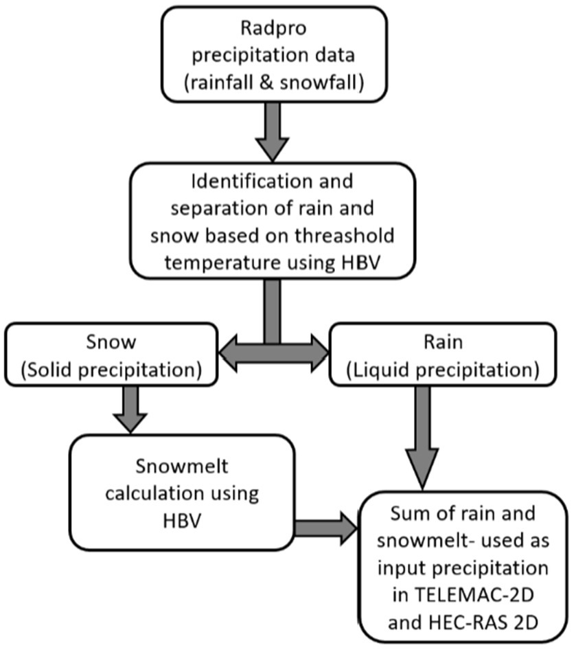
Figure 4. Flow chart for the methodology used in this research study.

2.2.5 Curve number method

The CN method is an empirical method which is commonly used to estimate the infiltration or direct runoff from rainfall excess in a particular catchment. The equation to calculate the direct runoff depth is as follows:

$Q=\{\begin{array}{l}0\mathit{\text{for}}P\le I_a\\ \frac{{\left(P-I_a\right)}^2}{P-I_a+S}\mathit{\text{for}}P>I_a\end{array}\text{ (7)}$

where Q (mm) is the direct runoff depth, P (mm) is the event rainfall depth, S (mm) is the potential maximum retention, and I_a is the initial abstraction or the amount of water lost before the runoff starts. In the current study, it is assumed as I_a = 0.2S. Curve number is a dimensionless parameter which depends on catchment’s hydrologic soil group, moisture condition, and land use. It is related to the above equation in the following way:

$\begin{array}{ll}S=24.5\left(\frac{100}{CN}-10\right)& (8)\end{array}$

CN varies from 30 to 100, where CN = 100 indicates no infiltration (high runoff) and lower CN values indicate higher infiltration (lower runoff). As shown in the CN equation, the runoff is generated only after the initial abstraction has been completed. Nonetheless, this method does not anticipate infiltration rate; instead, it predicts cumulative infiltration. In addition, time and rainfall intensity are not considered. As a result, this method is not the best for the areas in karst topography and for the areas containing the type of soils where a significant proportion of the flow is subsurface flow rather than direct runoff. Spatially distributed Manning’s roughness and CN values were used (Table 1) in both the models which were based only on the land cover data because soil information was not available for the catchment. Steep slope correction for CN values was applied in the T2D simulations considering the mountainous catchment using the following formula (Huang et al., 2006):

$\begin{array}{ll}CN{\left(II\right)}_{\alpha }=CN\left(II\right)\left(\frac{322.79+15.63\alpha }{\alpha +323.52}\right)& (9)\end{array}$

Here, $CN\left(II\right)$ represents the CN value corresponding to a $AMC\left(II\right)$, the normal antecedent moisture condition, while $\alpha$ denotes the terrain slope in m/m, ranging from 0.14 to 1.4 m/m. The $CN\left(II\right)$ values may experience an increase of up to 6% for $\alpha$ = 1.4 (Ligier, 2016).

2.2.6 Green-Ampt and green-Ampt redistribution method

In contrast to the CN method, the GA method is a physically based model. The rate of infiltration varies with time depending on the soil properties (Ogden and Saghafian, 1997). The CN method assumes an initial abstraction before the runoff starts, the GA model assumes that the runoff starts only when the rainfall rate is more than the infiltration rate. The GA approach assumes a sharp boundary between wet and dry soil, and the water potential varies with water content on the wetting front in the dry soil (Green and Ampt, 1911). To calculate the infiltration rate (f), the basic GA equation is as follows:

$\begin{array}{ll}f=K_S\left(1+\frac{\psi {\theta }_d}{F}\right)& (10)\end{array}$

Here, K_S is the saturated hydraulic conductivity, Ψ is the suction head, θ_d is the difference between the saturated water content (θ_S) and the initial soil water content (θ_i), and F is the cumulative infiltration. The depth of the wetting front (Z) is presented as F/θ_d. It is important to notice that the actual infiltration rate is the minimum of the rainfall intensity, and the infiltration rate calculated in the above equation.

The GA approach is suitable for reproducing single peak flow events where the effects of evapotranspiration and unsaturated gravity-driven flow are negligible. On the other hand, it is crucial to consider the soil moisture redistribution to accurately model sustained flow flood events caused by multi-storm rainfall. Two wetting fronts may be considered for such events and the Green-Ampt Redistribution (GAR) method is used to simulate the soil moisture recovery during a rainfall hiatus period. The basic GA method depends on four parameters, namely, saturated hydraulic conductivity (K_S), suction head (Ψ), initial (θi) moisture content, and saturated (θs) moisture content, whereas the GAR method considers two additional parameters, namely, residual moisture content (θ_r) and the pore size distribution index (λ). A rainfall hiatus period starts when the saturated hydraulic conductivity K_s is more than the rainfall. During this hiatus period, the soil moisture content starts to decrease and this change in the moisture content (θ₀) for the redistribution process is calculated as follows:

$\begin{array}{ll}\frac{d{\theta }_d}{dt}=\frac{1}{Z_0}\left\{f-E_{v,0}-K_i-\left[K_0+\frac{K_{S}G\left({\theta }_{i,}{\theta }_0\right)}{Z_0}\right]\right\}& (11)\end{array}$

where Z₀ is the depth to the wetting front given as F₀/(θ₀ − θ_i), E_v,0 is the evapotranspiration rate, K_i, K_S, and K₀ are the unsaturated hydraulic conductivities corresponding to initial θ_i, the saturated θ_S, and a moisture content of θ₀, respectively. G (θ_i, θ₀) is integral of the capillary drive through the saturated front which is computed as follows:

$\begin{array}{ll}G\left({\theta }_i,{\theta }_0\right)=\psi \frac{{\mathrm{\Theta }}_0^{3+\frac{1}{\lambda }}-{\mathrm{\Theta }}_i^{3+\frac{1}{\lambda }}}{1-{\mathrm{\Theta }}_i^{3+\frac{1}{\lambda }}}& (12)\end{array}$

where Θ is the relative water content. The main benefit of using the GAR method is that it takes into account the variation of rainfall excess intensity over time, a feature which is absent in the CN method. However, the calibration of GAR method depends on the availability of soil data, and it is a tedious and time-consuming process because of the large number of parameters and long simulation run-time in the hydrodynamic models. Therefore, to test the influence of the GAR parameters, a sensitivity analysis was done on a smaller model of only two cells.

2.2.7 Measures of accuracy

Pearson’s correlation coefficient (Pearson, 1897) and Nash–Sutcliffe Efficiency Index (Nash and Sutcliffe, 1970) were used as the measures of accuracy for the model results. The formulas for both are described below:

(a) Pearson’s correlation coefficient (R²)

It is the ratio of the mean square error to the potential error. The value ranges from 0 to 1, where 1 represents a perfect fit and 0 represents no fit. It is calculated using the following formula:

$\begin{array}{ll}{R}^2=\frac{{{\displaystyle \sum }}_{i=1}^n\left(Q_{obs}-Q_{ob{s}_m}\right)\left(Q_{sim}-Q_{si{m}_m}\right)}{\sqrt{{{\displaystyle \sum }}_{i=1}^n{\left(Q_{obs}-Q_{ob{s}_m}\right)}^2.{{\displaystyle \sum }}_{i=1}^n{\left(Q_{sim}-Q_{si{m}_m}\right)}^2}}& (13)\end{array}$

In this equation:

$R^2$ represents the Nash–Sutcliffe Efficiency Index;

$n$ is the total number of observations;

$Q_{obs}$ denotes the observed values;

$Q_{sim}$ represents the predicted values;

$Q_{ob{s}_m}$ signifies the mean of the observed values; and

$Q_{si{m}_m}$ signifies the mean of the simulated values.

(b) Nash–Sutcliffe Efficiency Index (NSE)

Nash–Sutcliffe Efficiency (NSE) Index is the absolute difference between observed and simulated values, which is then normalized by the variance of the observed discharge to remove any bias. In case of a perfect model, the estimated error value is 0, and hence, the NSE is 1. On the contrary, the NSE is 0 if the model produces an estimation error-variance equal to the observed time series. It is calculated using the following formula:

$\begin{array}{ll}NSE=1-\frac{{{\displaystyle \sum }}_{i=1}^n{\left(Q_{obs}-Q_{sim}\right)}^2}{{{\displaystyle \sum }}_{i=1}^n{\left(Q_{ob\mathrm{s}}-Q_{ob{s}_m}\right)}^2}& (14)\end{array}$

In this equation:

$NSE$ represents the Nash–Sutcliffe Efficiency Index;

$n$ is the total number of observations;

$Q_{obs}$ denotes the observed values;

$Q_{sim}$ represents the predicted values; and

$Q_{ob{s}_m}$ signifies the mean of the observed values.

3 Results and discussion

3.1 Calibration and single-storm flood events

The models are calibrated by varying the CN values and the roughness for different land covers (Table 1) to fit the simulated hydrograph for single storm events to the observations from the measurement station in the river (Figure 1). During the calibration process, when the same roughness and CN values were used in HR2D as in T2D, the runoff was lower (Pilotti et al., 2020), and the peak flow was not captured for event A by HR2D, as shown in Figure 5. Hence, the CN values were increased, and roughness was decreased to reproduce the peak flow in HR2D. Consequently, the time to the peak flow was earlier for HR2D. Moreover, it was also observed in a study by Zeiger and Hubbart (2021), where the Manning roughness was adjusted and decreased with 25% and down to 75% which was not physically realistic for their study area. To reproduce the peak in HR2D, more flow volume and a delayed peak were needed. Since the mesh size also controls the runoff volume (Godara et al., 2023b), the cell size for the catchment was decreased to 50 m, which increased the runoff volume. Afterward, Manning’s roughness values were increased to delay the peak which resulted in a good calibration of peak flow and timing for event A (Figure 5). One reason for different results from the two models for the same CN and Manning’s n values may be the steep slope correction applied in T2D as per the formula given in Equation (9), which increases the CN value based on the slope at the location. For event B in the same Figure 5, the mesh resolution was the same (5 m by 5 m and 100 m by 100 m); as in T2D (except the breaklines in HR2D), only the CN and roughness values were adjusted to reproduce the peak flow. These two flow events were induced by only single-storm rainfall events without any contribution of snowmelt.

Figure 5

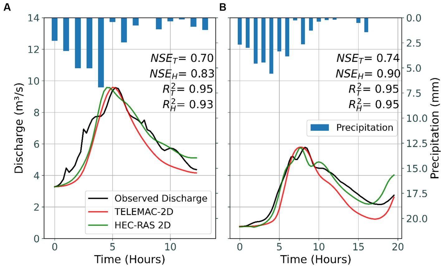
Figure 5. Observed discharge (black) and results from T2D (red) and HR2D (green) simulations. Both the models struggled to capture the initial rising part of the flood hydrograph in event A, but the recession part was better simulated by HR2D than by T2D in both the events.

The results show that the recession part is better simulated by HR2D than T2D in both the events, but both the models are struggled to capture the initial rising part of the flood hydrograph in event A. Similar results were observed in a study by Vu et al. (2015) for T2D flood inundation modeling, where the highest agreement between the modeled results and observations is for the peak flow conditions, not for pre- and post- flood conditions even for the flood extent. Reason behind a higher and therefore a better recession limb in HR2D can be the finer mesh in HR2D, which influence the overall volume under the curve of a hydrograph and a higher roughness, delaying and distributing the flow and keeping the volume higher until the end of simulations. A dam-break wave propagation study in a moderately steep valley was done by Pilotti et al. (2020) using HR2D version 5.0.7 and then compared the results with T2D version 7.0. They observed a slightly steeper rising limb and an early peak of the hydrograph in both models, which aligns with the findings of this study. However, they observed a milder recession limb compared to the observed one. However, the NSE values were quite similar. For this study, Nash–Sutcliffe efficiency and Pearson Correlation Coefficient values for T2D and HR2D are shown in Figure 5.

3.2 Mesh grid cells and simulation run-times

HR2D uses square shaped grid cells while T2D uses triangular shaped grid cells in the mesh. For the same length of the cell edges in the catchment, T2D gave more stable results as compared with HEC-RAS. One possible explanation for this can be the triangular shape of the grid cells instead of the square shape in HR2D which makes almost double the number of grid cells in T2D than in HR2D (Figure 2). Furthermore, HR2D took approximately five times longer simulation run-time as compared with T2D for the same set of parameters. T2D can run the simulation on eight core processors at the same time, showing the usage of 100% CPU capacity of the computer in task manager. HR2D also has an option to select the number of cores to be used (Goodell, 2016). Simulation run-time was tested by using 8, 16 and all available cores, but still, the task manager shows only approximately 60% of the CPU capacity usage during the simulations. This could be the reason for longer simulation times in HR2D. However, we refer to an article by Kleinschmidt Group (Goodell, 2016), to understand the utilization of a computer’s CPU by HR2D. Another reason for a longer simulation run-time in HR2D is the irregular shape of the grid cells along the steep sections in the catchments (Figure 3A, right).

Some artificial sinks were observed at the end of the HR2D simulations (David and Schmalz, 2021) and a significant amount of water was trapped in there (Figure 3A, right), which resulted in a lower runoff volume in the initial stages of the calibration. Unlike HR2D, T2D did not have any such problem of discontinuous flow or artifacts at extreme steep slopes. To remove these artifacts in HR2D, the mesh was refined in those particular areas by introducing breaklines (Figure 3B, left), which resulted in an increased runoff volume, peak flow, and simulation run-time. Even after the refined mesh in these areas, water was still trapped in very small point locations with extremely steep slopes (Figure 3B, right), which was difficult to remove.

The resulting flow did not seem continuous for the steeper sections of the river. One possible reason for the flow discontinuity in HR2D could be the way in which the model fills the grid cells with water. The cells are filled according to a stage–volume relationship and it starts filling up the cell from the deepest part of the cell. Low flow or long time-steps can lead to a visual impression of discontinuity even if the wetted areas of the cells are continuous (Goodell, 2015). Moreover, the acceleration term in the full momentum equation cannot be neglected in such a steep terrain. Therefore, full momentum shallow water equation set was used which gave a more continuous flow and stable results for these steeper sections in HR2D. Even after using the SWE-ELM with 1 s of computation interval, the flow was discontinuous at a small section of the river where there was a sudden vertical drop. The channel was modified at this location to smoothen the drop (Figure 6) and the flow became continuous. On the other hand, there was not such a discontinuity problem in T2D results because T2D calculates the values at the nodes of the triangular mesh elements and distributes evenly inside the grid cell. Hence, no discontinuity problem was observed inside the cells.

Figure 6

Figure 6. Original (A) and the modified river (B) at the steep sections.

3.3 Multi-storm flood events with sustained flow

Figure 7 shows results from HBV hydrological model and T2D and HR2D HDRRM models for a flood event occurred by multiple storms. T2D simulations were run using the CN method, and HR2D simulations were run using CN and GAR methods. The results from the GAR method in HR2D (green curve in Figure 7) show that the flow between the two peaks was not reproduced, and the second peak is way higher than that of the observed flow.

Figure 7

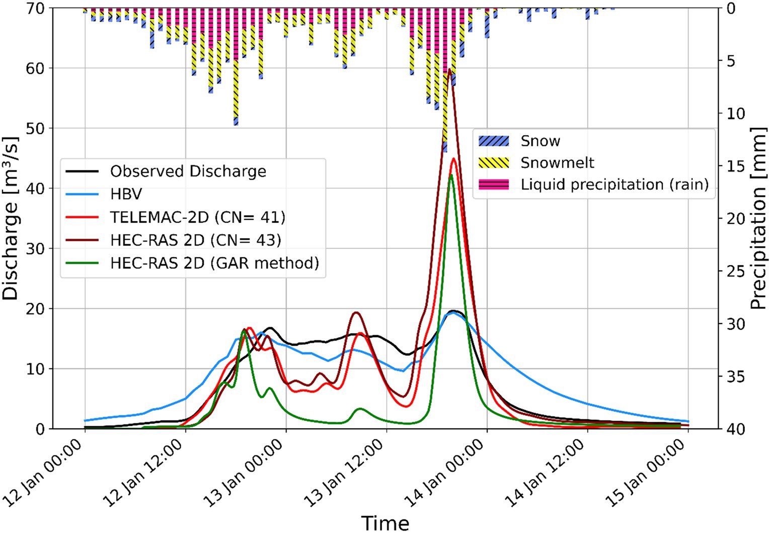
Figure 7. Multi-storm flood event with two peaks induced by a rain-on-snow event. Observed discharge (black) and results from the hydrologic model HBV (blue) and hydrodynamic rainfall-runoff models T2D (red) and HR2D from CN (maroon) and GAR methods (green).

Hydraulic conductivity (K_S) affects the resulting runoff volume throughout the entire event. When the conductivity is less than the rainfall rate throughout the event, the infiltration rate decreases exponentially to reach the infiltration rate equal to the hydraulic conductivity. During the rainfall hiatus period (when K_S > rainfall rate), the infiltration rate is approximately equal to the K_S (which is higher than the rainfall). As explained in section 2.2.6, the actual infiltration will be minimum of the infiltration rate [f(t)] and the rainfall rate. Hence, most of the rain infiltrates and the sustained flow between the two storms are not reproduced. For the event as shown in Figure 7, the minimum precipitation rate between the two rainstorms is approximately 5 mm/h; so, to maintain the non-hiatus period and the flow between the two storms, the K_S should always be less than 5 mm/h. However, such a low value of hydraulic conductivity results in higher peak flows for both the storms. Hence, a higher value of the hydraulic conductivity, 10 mm/h is used to calibrate the model at least for the first peak. Consequently, this high value of conductivity leads to a lower flow between the peaks.

The simulated extremely high peak flow for the last storm in this event is because even though the infiltration rate decreases with the time, the soil moisture recovery was not enough prior to the following heavy rainfall. Attempts were made to calibrate this peak, but the model results were not very sensitive to the two GAR parameters, which are responsible for the recovery of the infiltration rate. A sensitivity analysis for all the GAR parameters was done to better understand the effect of these parameters. The results are shown in the subsequent section. The GAR parameters used for the event, as shown in Figure 7, are:

Wetting Front Suction = 100 mm;

Saturated Hydraulic Conductivity = 10 mm/h;

Initial Soil Water Content = 0.1;

Saturated Soil Water Content = 0.8;

Residual Soil Water Content = 0.02;

Pore-size Distribution Index = 0.7;

Additionally, there always exists a return flow component. In such a steep catchment with shallow soils, the contributing return flow is even higher to the river. The water which is infiltrated into the shallow soils is permanently lost from the T2D and HR2D models because a groundwater model is not incorporated into these HDRR models, and thereby, the infiltrated water does not contribute to the runoff flow in the river. However, it is well established that in reality, the infiltrated water significantly contributes to the runoff in thin soils with steep slopes. Therefore, this problem of low flow between the storms can be resolved by introducing a delay mechanism that enables the infiltrated water to resurface and contribute to the runoff between the two precipitation events. This is precisely what is implemented in the soil routine of the HBV model, where the release of water from the soil routine to the runoff is followed by a retention delay that mimics the subsurface water dynamic. In the HBV model, the sub-surface water that is withheld by the soil routine is available for the model for future time-steps, which ensures continued runoff generation during the entire events with sustained flow. This contrasts with the T2D and HR2D models, where the infiltrated water is lost and not included in the runoff at later stages.

Furthermore, it is also shown in Figure 7 that CN method and GAR method did not give similar result for the flow between two peaks. The reason behind this is that the CN method has a constant infiltration rate, but in the GAR method, the infiltration rate varies with time based on the relationship between precipitation rate and hydraulic conductivity. The actual infiltration rate in the GAR method is the minimum out of the precipitation rate and the infiltration rate as calculated by Equation (10). Since the precipitation rate is lower than the hydraulic conductivity, most of the precipitation infiltrates, in contrast to the CN method, which has a constant infiltration. Therefore, the flow between the two peaks is higher for the CN method than for GAR method, as shown in Figure 7.

Figure 8 shows the cumulative precipitation, infiltration, and excess depth for a grid cell from the HR2D simulation using both CN and GAR infiltration methods for the event, as shown in Figure 7. The results show that the difference between the precipitation depth and the excess depth is equal to the infiltration depth, which means if the infiltrated water could contribute to the runoff as a return flow, the flow between the storms would have been higher and sustained. Figure 8 also shows how the infiltration rate in the GAR method varies and confirms that it is higher in the GAR method than in the CN method for the period between the two storms (roughly between 12 January 20:00 and 13 January 08:00) as claimed in the previous paragraph.

Figure 8

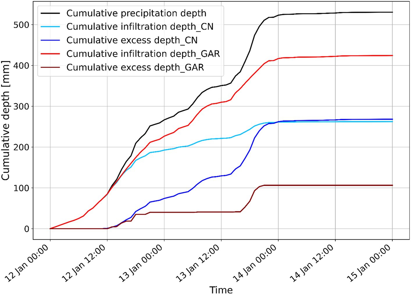
Figure 8. Cumulative precipitation, infiltration depths, and excess depths for a grid cell from HR2D simulation using CN and GAR methods for the event, shown in Figure 7.

3.4 Sensitivity analysis of GAR method parameters

Based on the experience from the multipeak event (Figure 7) and the application of the CN method in T2D in the earlier study (Godara et al., 2023a), it is evident that the CN method has limitations to produce satisfactory results for flood events with multiple peak flows. Therefore, the HR2D model with the GAR infiltration method was tested to simulate such events because GAR has a variable infiltration rate unlike the CN method. In theory, the GA model should be able to recover the infiltration capacity during dry periods (Brunner, 2020), as also explained in the methods section, and should overcome the limitations of the CN method in T2D. However, this was not the case as shown in the previous section. Hence, sensitivity analysis of the GAR method parameters was done to understand why this method is not be able to reproduce multi-peak floods and understand the effect of each parameter. The analysis was done on a smaller area with two cells for faster simulations.

The parameters for original GA method are Wetting Front Suction (Ψ), Saturated Hydraulic Conductivity (K_S), Initial Soil Moisture Content (θi), and the Saturated Soil Moisture Content also called the Porosity (θs). Two additional parameters making it the GAR method are Residual Soil Moisture Content (θr) and Pore-size Distribution Index (λ). These six parameters were used for the flood events triggered by multi-storm precipitations. The analysis shows that the results are most sensitive to the four parameters that are used in the basic GA method, whereas the additional two parameters from the GAR method do not have a large effect on the results. The subsequent sub-sections show the effect of each parameter in detail.

3.4.1 Saturated hydraulic conductivity (K_S)

Three values of hydraulic conductivity K_S = 2, 5 and 10 mm/h were used in a smaller model to check the sensitivity using a constant precipitation rate of 10 mm/h. All the other parameters were kept constant. The results in Figures 9A,B show that if the hydraulic conductivity is more than or equal to the precipitation rate (10 mm/h in this case), all the water infiltrates and there is no excess water left as surface runoff. Additionally, as the difference between conductivity and precipitation rate increases, infiltration decreases exponentially to reach an infiltration rate equal to the hydraulic conductivity.

Figure 9

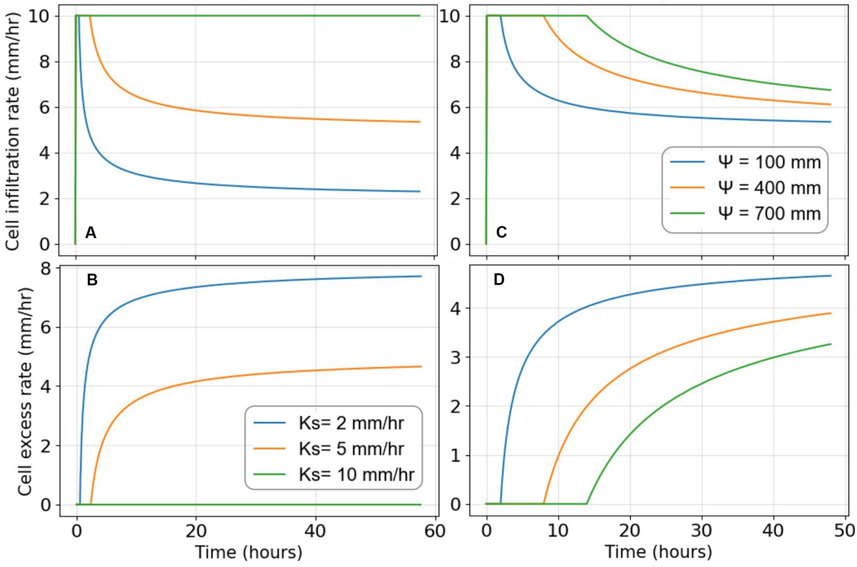
Figure 9. Cell infiltration and excess rate for different saturated hydraulic conductivity (A,B) and suction heads (C,D) using precipitation rate of 10 mm/h.

3.4.2 Suction head (Ψ)

A constant precipitation rate of 10 mm/h was used over two cells to check the sensitivity of suction head for three values Ψ = 100, 400, and 700 mm keeping the other parameters constant. The results in Figures 9C,D show that the higher the suction head, the higher the infiltration rate. Consequently, the excess flow rate is lower, and runoff starts later in time for a higher suction head.

3.4.3 Moisture deficit (θd = θs – θi)

Various values of initial (θi) and saturated (θs) moisture content were tested, and it was found that the results were sensitive to the difference between the two moisture contents (moisture deficit (θd)), instead of the initial and saturated moisture contents separately. Constant precipitation rate of 10 mm/h, K_S = 5 mm/h, and Ψ = 700 mm was used over the cells to check the sensitivity. Figures 10A,B shows that the higher the moisture deficit, the larger the infiltration rate, and the surface runoff start later in time. The results also show the same curves for the scenarios, where the value of moisture deficit is same, even though the initial and saturated moisture content values are changed.

Figure 10

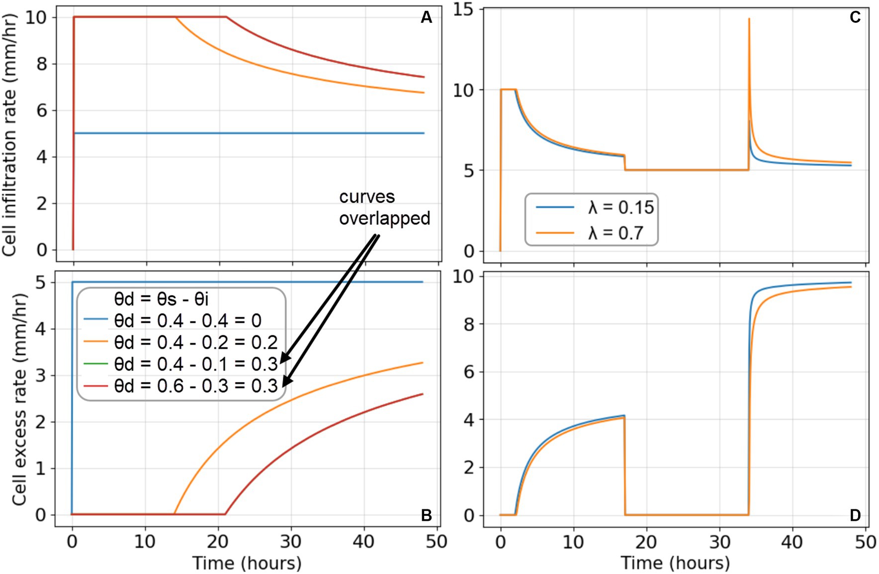
Figure 10. Cell infiltration and excess rate for different moisture deficit values (A,B) and the maximum and minimum values of pore size distribution index (C,D).

3.4.4 Residual water content (θr)

Residual moisture content θr is the one of the parameters that affects the shape of the hydrograph after the rainfall hiatus period (GAR method). Therefore, a rainfall event with varying intensities 10 mm/h, 5 mm/h and 15 mm/h was used in this case as shown in Figure 11A. Keeping the initial and saturated moisture contents constant along with the rest of the parameters, residual moisture content was varied from minimum 0.01 to maximum 0.1 (as per the Table 4 in Brunner, 2020). Figures 11B,C shows that the higher the residual moisture content, the lower the infiltration rate after the rainfall hiatus period and the higher the second peak, but the results are not very sensitive to this GAR parameter.

Figure 11

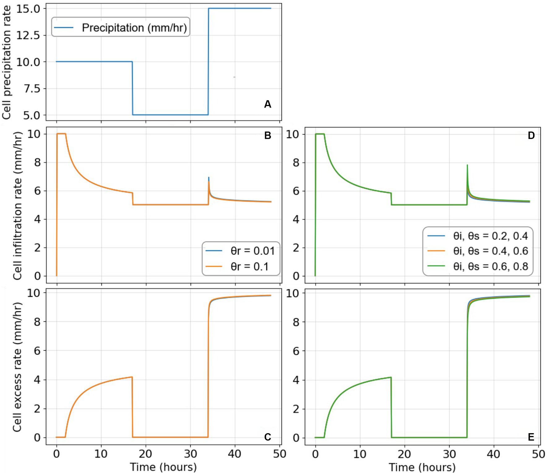
Figure 11. Precipitation (A) used for the sensitive analysis of redistribution parameters, (B,C) show cell infiltration and excess rate for the various values of the residual moisture contents. (D,E) Show the same for various combinations of initial and saturated moisture contents, keeping the same value of moisture deficit.

Different combinations of the initial and saturated moisture contents were also tested for sensitivity (Figures 11D,E), keeping the same values for residual moisture content and moisture deficit. The results in Figure 11 show that the effect is only on the second peak, but overall, the results are not very sensitive.

3.4.5 Pore size distribution index (λ)

Keeping all the parameters constant and using the same varying precipitation as above, the pore size infiltration index was changed to the maximum and minimum values of λ (0.7 and 0.15) (Brunner, 2020). The results in Figures 10C,D show that higher the pore size index, the lower the first and second peak flows, but the second peak is influenced more, although the overall results are not very sensitive to the value of pore size distribution index.

The outcomes of the sensitivity analysis reveal that the GAR method behaves as anticipated and produces the expected results. Nevertheless, it is still not be able to simulate longer flood events correctly. This discrepancy suggests that the probable cause for the inability to reproduce multi-storm and prolonged flood events lies in the loss of infiltrated water and the absence of a subsurface water module in HDRR models (T2D and HR2D).

3.5 Velocity and inundation maps

Figures 12, 13 show velocity and inundation maps from the models T2D and HR2D for event B, as shown in Figure 5. Finer mesh (3 m × 3 m) was introduced along the steep section of the river in both the models to capture the terrain with better accuracy. The results show that the inundation areas are approximately the same from both the models except that T2D shows continuous regions, whereas HR2D shows that it scattered at some locations outside the river reach. This discrepancy in the results was also observed in a study (Orozco et al., 2023), where the two models were compared for levee breach analysis. This difference is because T2D distributes the water evenly across each grid cell calculated from the values at nodes of the grid cell. In contrast, HR2D has sub-grid technology, preserving the detailed information of topography within the grid cells, resulting in partially wet cells and more distinctly defined floodplain areas. This feature enhances result precision, providing a more comprehensive understanding of the area and water behavior during both modeling and post-processing stages. Because of this difference, the extent of the inundation seems more continuous from T2D simulations as compared with that from HR2D simulations.

Figure 12

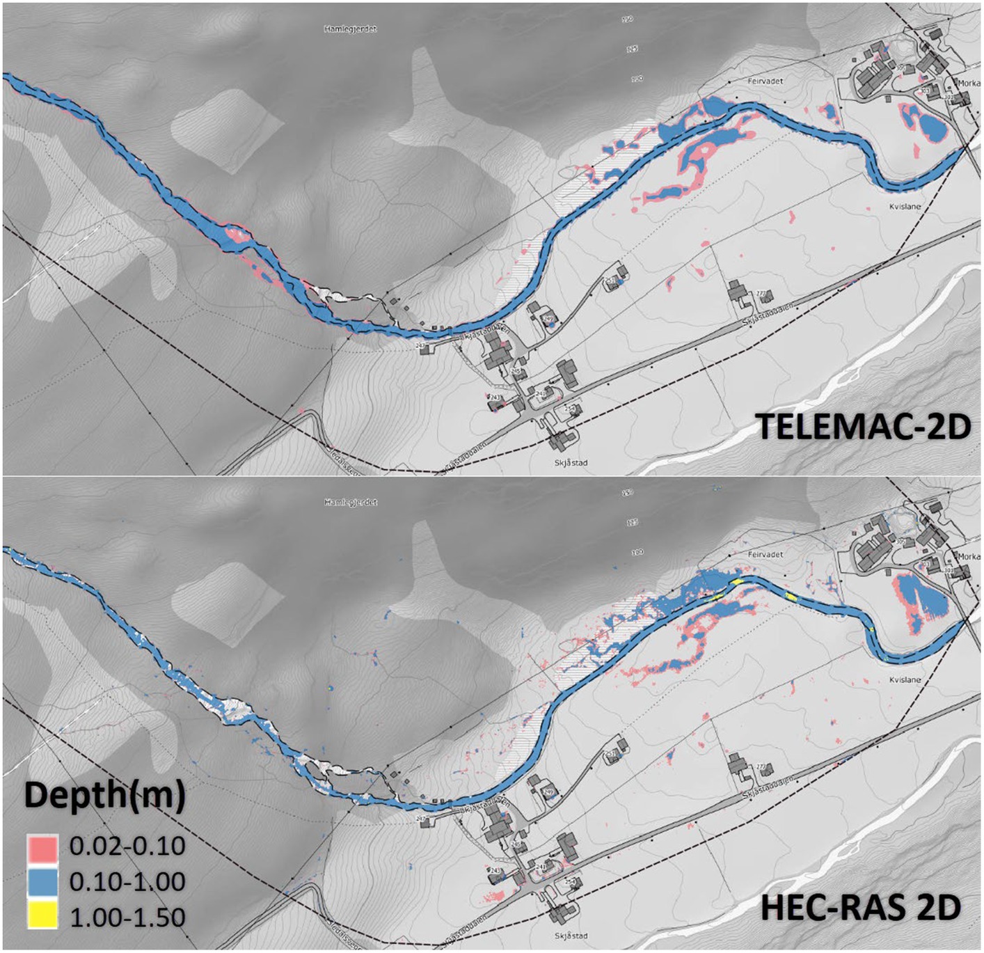
Figure 12. Water depth results from T2D and HR2D simulation results for event B in Figure 5.

Figure 13

Figure 13. Velocity results from T2D and HR2D simulation results for event B in Figure 5.

Furthermore, the results show that maximum water depth and maximum velocity values are higher in HR2D than T2D. The reason behind excessively high maximum values can be the steep slope of the catchment, in which HR2D probably is not designed to accommodate. Some locations in the catchment have vertical drops, and even after refining the mesh, tiny ponds were formed similar to the ones shown in Figure 3A, with a high value of depth at the location and velocity at these vertical drops.

In general, higher values of velocity were calculated by HR2D, as shown in Figure 13. Figure 14 shows the velocity distribution along the centerline of the river stretch shown in depth and velocity maps, along with the slope in the same river stretch. The figure shows that HR2D calculates higher velocities than T2D along the steeper sections, especially when the slope is more than approximately 20 degrees which is way above the suggested maximum slope values for HR2D (Brunner, 2016). However, velocities at the flatter sections were mostly similar from both the models, as shown in the most right and the most left river sections in Figures 13, 14.

Figure 14

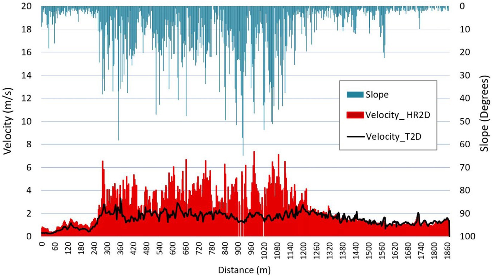
Figure 14. Slope (blue clustered columns on the secondary axis) and velocity distribution (red clustered columns from HR2D and black line from T2D) along the centerline of the river stretch shown in Figures 12, 13.

4 Conclusion

The goal of this study was to compare the two hydrodynamic rainfall-runoff models TELEMAC-2D and HEC-RAS 2D for their rain-on-grid technique and, especially, to reproduce long-duration flood events with sustained flow between flow peaks. Sensitivity analysis of the GAR infiltration method parameters was also done to understand the behavior of models to simulate such events. The study has also explored their strengths and weaknesses in terms of calibration process, simulation run-time, input file preparation, and post-processing of results. Use of CN infiltration method in T2D and HR2D was compared, as well as the GAR infiltration method in HR2D was tested in the RoG technique.

Peak flow for single storm flood events was reproduced by both the models. The results show that this fully integrated hydrodynamic rainfall-runoff modeling with RoG tool can only be used for flash floods in small rivers not for a big river flood with long duration floods, where significant amount of water infiltrates. The plots from this study and our previous studies on this topic conclude that this type of models is good to simulate single-storm flood events limited to 10–15 h of duration or to the flood events where it is sure that the infiltrated water percolates to the deep groundwater flow, and there is no chance of subsurface return flow. For the longer duration single-storm floods, the recession part is not simulated well. Similarly, for multi-storm events, this tool fails to accurately capture the flow dynamics between the storms. Although, the sensitivity analysis of the GAR parameters on a multi-storm event gave expected results, but none of the HDRR models with CN or GAR infiltration method could simulate this. The main reason for this limitation is the lack of a soil routine module which can include the contribution of delayed subsurface water to resulting flow hydrograph. The addition of a subsurface water routine inside the HDRR models should be one of the future works. Furthermore, the resulting inundation maps from the models should be compared with the observed inundation maps, since these were not available for the area and flood events used in this study.

Nonetheless, the tool developed in this research study is applicable for analyzing flash floods and their consequences in steep catchments. Since flash floods are expected to increase in future due to increased short-duration, high-intensity precipitation events, this model will hold direct relevance and significance in future assessments of climate change impacts in terms of flash floods. The results from this study may help the engineers and researchers to choose the suitable model for their purpose out of the two hydrodynamic rainfall-runoff models which have the option for modeling a steep catchment and river systems using rain-on-grid technique. Furthermore, these results can provide a useful tool for flood risk management, infrastructure planning, and risk and vulnerability analysis for flash floods using an appropriate rain-on-grid hydrodynamic model. The analysis can help the municipality and infrastructure planners to find critical locations in an area in terms of submergence, water depth, high velocities, and shear stresses.

Data availability statement

The raw data supporting the conclusions of this article will be made available by the authors, without undue reservation.

Author contributions

NG: Conceptualization, Data curation, Formal analysis, Investigation, Methodology, Software, Validation, Visualization, Writing – original draft, Writing – review & editing. OB: Conceptualization, Funding acquisition, Methodology, Project administration, Resources, Supervision, Writing – review & editing. KA: Conceptualization, Methodology, Supervision, Writing – review & editing.

Funding

The author(s) declare that financial support was received for the research, authorship, and/or publication of this article. This publication was part of the World of Wild Waters (WoWW) project number 949203100, which falls under the umbrella of the Norwegian University of Science and Technology (NTNU)’s Digital Transformation initiative.

Conflict of interest

The authors declare that the research was conducted in the absence of any commercial or financial relationships that could be construed as a potential conflict of interest.

Publisher’s note

All claims expressed in this article are solely those of the authors and do not necessarily represent those of their affiliated organizations, or those of the publisher, the editors and the reviewers. Any product that may be evaluated in this article, or claim that may be made by its manufacturer, is not guaranteed or endorsed by the publisher.

Footnotes

1. ^www.hoydedata.no

2. ^www.geonorge.no

References

Barredo, J. I. (2007). Major flood disasters in Europe: 1950–2005. Nat. Hazards 42, 125–148. doi: 10.1007/s11069-006-9065-2

Crossref Full Text | Google Scholar

Barton, A. J. (2019). Blue Kenue enhancements from 2014 to 2019. 26th TELEMAC-MASCARET User Conference, 15th to 17th October 2019, Toulouse.

Google Scholar

Basso-Báez, S., Mazzorana, B., Ulloa, H., Bahamondes, D., Ruiz-Villanueva, V., Sanhueza, D., et al. (2020). Unravelling the impacts to the built environment caused by floods in a river heavily perturbed by volcanic eruptions. J. S. Am. Earth Sci. 102:102655. doi: 10.1016/j.jsames.2020.102655

Crossref Full Text | Google Scholar

Bergström, S., and Forsman, A. (1973). Development of a conceptual deterministic rainfall - runoff model. Nord. Hydrol. 4, 147–170. doi: 10.2166/nh.1973.0012

Crossref Full Text | Google Scholar

Borga, M., Stoffel, M., Marchi, L., Marra, F., and Jakob, M. (2014). Hydrogeomorphic response to extreme rainfall in headwater systems: flash floods and debris flows. J. Hydrol. 518, 194–205. doi: 10.1016/j.jhydrol.2014.05.022

Crossref Full Text | Google Scholar

Bruland, O. (2020). How extreme can unit discharge become in steep Norwegian catchments? Hydrol. Res. 51, 290–307. doi: 10.2166/nh.2020.055

Crossref Full Text | Google Scholar

Brunner, G. W. (2002). Hec-ras (river analysis system). In North American water and environment congress & destructive water ASCE. 3782–3787.

Google Scholar

Brunner, G. W. (2016). HEC-RAS river analysis system: hydraulic reference manual, version 5.0. Davis, CA, USA: US Army Corps of Engineers–Hydrologic Engineering Center. 547.

Google Scholar

Brunner, G. W. (2020). HEC-RAS river analysis system: hydraulic reference manual, version 6.0 Beta. Davis, CA, USA: US Army Corps of Engineers–Hydrologic Engineering Center. 1–464.

Google Scholar

David, A., and Schmalz, B. (2021). A systematic analysis of the interaction between rain-on-grid-simulations and spatial resolution in 2d hydrodynamic modeling. Water (Switzerland) 13:2346. doi: 10.3390/w13172346

Crossref Full Text | Google Scholar

Engeland, K., Abdella, S. Y., Azad, R., Arrturi Elo, C., Lussana, C., Tadege Mengistu, Z., et al. (2018). Use of precipitation radar for improving estimates and forecasts of precipitation estimates and streamflow. 20th EGU General Assembly, EGU2018, Proceedings from the Conference, 4–13 April, 2018, Vienna.

Google Scholar

Feng, B., Zhang, Y., and Bourke, R. (2021). Urbanization impacts on flood risks based on urban growth data and coupled flood models. Nat. Hazards 106, 613–627. doi: 10.1007/s11069-020-04480-0

Crossref Full Text | Google Scholar

Godara, N., Bruland, O., and Alfredsen, K. (2023a). Modelling flash floods driven by rain-on-snow events using rain-on-grid technique in the hydrodynamic model TELEMAC-2D. Water 15:3945. doi: 10.3390/w15223945

Crossref Full Text | Google Scholar

Godara, N., Bruland, O., and Alfredsen, K. (2023b). Simulation of flash flood peaks in a small and steep catchment using rain-on-grid technique. J. Flood Risk Manag. 16, 1–14. doi: 10.1111/jfr3.12898

Crossref Full Text | Google Scholar

Goodell, C. (2015). 2D troubleshooting – fragmented inundation. Available at: https://www.kleinschmidtgroup.com/ras-post/2d-troubleshooting-fragmented-inundation/

Google Scholar

Goodell, C. (2016). Optimizing your Computer for Fast HEC-RAS modeling. Available at: https://www.kleinschmidtgroup.com/ras-post/optimizing-your-computer-for-fast-hec-ras-modeling/

Google Scholar

Green, W. H., and Ampt, G. A. (1911). Studies on Soil Physics. The Journal of Agricultural Science, 4, 1–24. doi: 10.1017/S0021859600001441

Crossref Full Text | Google Scholar

Hariri, S., Weill, S., Gustedt, J., and Charpentier, I. (2022). A balanced watershed decomposition method for rain-on-grid simulations in HEC-RAS. J. Hydroinf. 24, 315–332. doi: 10.2166/hydro.2022.078

Crossref Full Text | Google Scholar

Huang, M., Gallichand, J., Wang, Z., and Goulet, M. (2006). A modification to the soil conservation service curve number method for steep slopes in the loess plateau of China. Hydrol. Process. 20, 579–589. doi: 10.1002/hyp.5925

Crossref Full Text | Google Scholar

Jha, L. K., and Khare, D. (2016). Glacial lake outburst flood (GLOF) study of Dhauliganga basin in the Himalaya. Cogent Environ. Sci. 2:1249107. doi: 10.1080/23311843.2016.1249107

Crossref Full Text | Google Scholar

Johnson, J. P. L., Whipple, K. X., and Sklar, L. S. (2010). Contrasting bedrock incision rates from snowmelt and flash floods in the Henry Mountains, Utah. Geol. Soc. Am. Bull. 122, 1600–1615. doi: 10.1130/B30126.1

Crossref Full Text | Google Scholar

Kishore, N., and Rishi, S. (2014). Morphometry and geomorphological investigations of the Neugal watershed, Beas River basin, Kangra District, Himachal Pradesh using GIS tools. J. Environ. Earth Sci. 4, 78–86.

Google Scholar

Li, L., Pontoppidan, M., Sobolowski, S., and Senatore, A. (2020). The impact of initial conditions on convection-permitting simulations of a flood event over complex mountainous terrain. Hydrol. Earth Syst. Sci. 24, 771–791. doi: 10.5194/hess-24-771-2020

Crossref Full Text | Google Scholar

Ligier, P. (2016). Implementation of a rainfall-runoff model in TELEMAC-2D. In: Bourban, Sébastien (Hg.): Proceedings of the XXIIIrd TELEMAC-MASCARET User Conference 2016, 11 to 13 October 2016, Paris, France. Oxfordshire: HR Wallingford. S. 13–19.

Google Scholar

Lin, Q., Lima, P., Steger, S., Glade, T., Jiang, T., Zhang, J., et al. (2021). National-scale data-driven rainfall induced landslide susceptibility mapping for China by accounting for incomplete landslide data. Geosci. Front. 12:101248. doi: 10.1016/j.gsf.2021.101248

Crossref Full Text | Google Scholar

Liu, T., Wang, Y., Yu, H., and Chen, Y. (2022). Using statistical functions and hydro-hydraulic models to develop human vulnerability curves for flash floods: the flash flood of the Taitou catchment (China) in 2016. Int. J. Disast. Risk Reduct. 73:102876. doi: 10.1016/j.ijdrr.2022.102876

Crossref Full Text | Google Scholar

Maatar, F. E., Domeneghetti, A., and Brath, A. (2015). HEC-RAS 5.0 vs. TELEMAC-2D: a model comparison for flood-hazard and flood-risk estimation. EGU General Assembly, Held 12–17 April, 2015, Vienna.

Google Scholar

Maqtan, R., Othman, F., Wan Jaafar, W. Z., Sherif, M., and El-Shafie, A. (2022). A scoping review of flash floods in Malaysia: current status and the way forward. Nat. Hazards 114, 2387–2416. doi: 10.1007/s11069-022-05486-6

Crossref Full Text | Google Scholar

Marchi, L., Borga, M., Preciso, E., and Gaume, E. (2010). Characterisation of selected extreme flash floods in Europe and implications for flood risk management. J. Hydrol. 394, 118–133. doi: 10.1016/j.jhydrol.2010.07.017

Crossref Full Text | Google Scholar

Moraru, A., Pavlíček, M., Bruland, O., and Rüther, N. (2021). The story of a Steep River: causes and effects of the flash flood on 24 July 2017 in Western Norway. Water 13:1688. doi: 10.3390/W13121688

Crossref Full Text | Google Scholar

Nash, J. E., and Sutcliffe, J. V. (1970). River flow forecasting through conceptual models part I—a discussion of principles. J. Hydrol. 10, 282–290. doi: 10.1016/0022-1694(70)90255-6

Crossref Full Text | Google Scholar

Ogden, F. L., and Saghafian, B. (1997). Green and Ampt infiltration with redistribution. Water Resour. Res. 123, 386–393. doi: 10.1061/(ASCE)0733-9437(1997)123:5(386)

Crossref Full Text | Google Scholar

Orozco, A. N. R., Bertrand, N., Pheulpin, L., Migaud, A., and Abily, M. (2023). “Comparison between HEC-RAS and TELEMAC-2D hydrodynamic models of the Loire River, integrating levee breaches” in SimHydro 2023: New Modelling Paradigms for Water Issues?

Google Scholar

Pearson, P. K. (1897). Mathematical contributions to the theory of evolution.—on a form of spurious correlation which may arise when indices are used in the measurement of organs. Proc. R. Soc. Lond. 60, 489–498. doi: 10.1098/rspl.1896.0076

Crossref Full Text | Google Scholar

Pilotti, M., Milanesi, L., Bacchi, V., Tomirotti, M., and Maranzoni, A. (2020). Dam-break wave propagation in Alpine Valley with HEC-RAS 2D: experimental Cancano test case. J. Hydraul. Eng. 146, 1–11. doi: 10.1061/(asce)hy.1943-7900.0001779

Crossref Full Text | Google Scholar

Rangari, V. A., Umamahesh, N. V., and Bhatt, C. M. (2019). Assessment of inundation risk in urban floods using HEC RAS 2D. Model. Earth Syst. Environ. 5, 1839–1851. doi: 10.1007/s40808-019-00641-8

Crossref Full Text | Google Scholar

Sarker, S. (2022). A short review on computational hydraulics in the context of water resources engineering. Open J. Model. Simul. 10, 1–31. doi: 10.4236/ojmsi.2022.101001

Crossref Full Text | Google Scholar

Seneviratne, S. I., Zhang, X., Adnan, M., Badi, W., Dereczynski, C., Di Luca, S. G., et al. (2021). IPCC - climate change 2021: The physical science basis - chapter 11: Weather and climate extreme events in a changing climate. Cambridge: Cambridge University Press.

Google Scholar

Swanston, D. N. (1974). Slope stability problems associated with timber harvesting in mountainous regions of the Western United States. USDA For. Serv. Gen. Tech. Rep. PNW-21:21

Google Scholar

Sweeney, T. L. (1992). Modernized areal flash flood guidance. Springfield VA USA: NOAA technical memorandum NWS HYDRO, 44.

Google Scholar

TELEMAC-2D User Manual v8p2. (2020). 1 December 2020. Last accessed: 12 January 2024. https://gitlab.pam-retd.fr/otm/telemac-mascaret/-/raw/v8p5r0/documentation/telemac2d/user/telemac2d_user_v8p2.pdf

Google Scholar

Vázquez Conde, M. T., Lugo, J., and Guadalupe Matías, L. (2001). “Heavy rainfall effects in Mexico during early October 1999” in Coping with flash floods (Netherlands: Springer), 289–299.

Google Scholar

Vu, T., Nguyen, P., Chua, L., and Law, A. (2015). Two-dimensional hydrodynamic modelling of flood inundation for a part of the Mekong River with TELEMAC-2D. Br. J. Environ. Clim. Change 5, 162–175. doi: 10.9734/bjecc/2015/12885

Crossref Full Text | Google Scholar

Zeiger, S. J., and Hubbart, J. A. (2021). Measuring and modeling event-based environmental flows: an assessment of HEC-RAS 2D rain-on-grid simulations. J. Environ. Manag. 285:112125. doi: 10.1016/j.jenvman.2021.112125

PubMed Abstract | Crossref Full Text | Google Scholar

Zhang, G., Cui, P., Yin, Y., Liu, D., Jin, W., Wang, H., et al. (2019). Real-time monitoring and estimation of the discharge of flash floods in a steep mountain catchment. Hydrol. Process. 33, 3195–3212. doi: 10.1002/hyp.13551

Crossref Full Text | Google Scholar