Inverse problem assisted multivariate geostatistical model for identification of transmissivity fields

Groundwater models often require transmissivity (T) fields as an input. These T fields are commonly generated by performing univariate interpolation of the T data. This T data is derived from pumping tests and is generally limited due to the large costs and logistical requirements. Hence T fields generated using this limited data may not be representative for a whole study region. Groundwater models often require transmissivity (T) fields as an input. These T fields are commonly generated by performing univariate interpolation (using kriging, IDW etc.) of the T data. This T data is derived from pumping tests and is generally limited due to the large costs and logistical requirements. Hence, the T fields generated using this limited data may not be representative for the whole study region. This study presents a novel cokriging based methodology to generate credible T fields. Cokriging - a multivariate geostatistical interpolation method permits incorporation of additional correlated auxiliary variables for the generation of enhanced fields. Here abundantly available litholog derived saturated thickness data has been used as secondary (auxiliary) data given its correlation with the primary T data. Additionally, the proposed methodology addresses two operational problems of traditional cokriging procedure. The first operational problem is the poor estimation of variogram and cross-variogram parameters due to sparse T data. The second problem is the determination of relative contributions of primary and secondary variable in the estimation process. These two problems have been resolved by proposing a set of novel non-bias conditions, and linking the interpolator with a head based inverse problem solution for credible estimation of these parameters. The proposed methodology has been applied to Bist doab region in Punjab (India). Additionally, base line studies have been performed to elucidate the superiority of the proposed cokriging based methodology over kriging in terms of head reproducibility.

1 Introduction

Distributed groundwater flow models are being increasingly used for regional planning of groundwater development (McKinney and Lin, 1994; Marino, 2001; Bhattacharjya and Datta, 2005; Miller et al., 2009; Ghosh and Kashyap, 2012; Singh et al., 2016; Escriva-Bou et al., 2020; Zeinali et al., 2020; Maliva et al., 2021; Mamo et al., 2021; Izady et al., 2022; Bailey et al., 2023). These models invariably require values of transmissivity (T) at the spatial grid cells. Pumping tests can provide data of these values only at a limited number of locations due logistical difficulties and large expenses involved. The present practice for bridging this data gap is centered around two broad strategies viz. interpolation alone, or joining of interpolation with an inverse problem (IP) solution. The former practice involves interpolating cell values of T (or hydraulic conductivity) employing only the available measured values (Anderson et al., 2015; Dickson et al., 2019). The latter practice invokes the interpolator and also a flow model so that more information can be used to obtain better estimates of T using historical head measurements through the use of an optimizer (Yeh, 2015). Employing measured T values and historical head fields, it aims at producing hydraulically consistent T field that has better predictive capability, than would be obtained using T values alone.

Commonly used interpolation functions include finite element linked basis functions (Yoon and Yeh, 1976), spline, polynomial (Chapra and Canale, 2010; Yao et al., 2014; Adhikary et al., 2017), and geostatistical tools viz. kriging (RamaRao et al., 1995; Kitanidis, 1997; Oliver and Webster, 2015; Kavusi et al., 2020; Cui et al., 2021; Kapoor and Kashyap, 2021; Senoro et al., 2021; Panagiotou et al., 2022; Júnez-Ferreira et al., 2023) and cokriging (Aboufirassi and Mariño, 1984; Ahmed and de Marsily, 1987; Ahmed et al., 1988; Kitanidis, 1997; Wackernagel, 2003; Belkhiri et al., 2020; Zawadzki et al., 2021; Zhao et al., 2022; Christelis et al., 2023). The present study centers around cokriging, that is a multivariate form of the univariate geostatistical tool kriging (Kitanidis, 1997; Oliver and Webster, 2015). Kriging is the best linear unbiased interpolator of a regionalized stationary variable preserving its measured values. The interpolation is based upon the spatial statistics of measured values. The spatial statistics is estimated by a variogram which depicts auto-semivariance of the variable as a function of the separation distance. The interpolated value is expressed as a linear combination of the measured values, and the weights are estimated from the requirements of minimized mean square error and the unbiasedness of the interpolation.

Cokriging, based upon similar concepts, introduces an additional stationary regionalized secondary variable (B) that is a priori known to be correlated to the variable subjected to interpolation (termed as primary variable). The spatial statistics in this case are defined in terms of variograms of the primary and secondary variables, and cross-variogram between the primary and secondary variables. The latter describes the variation of cross-semivariance between T and B as a function of the separation distance. The interpolated value in this case is expressed as linear combination of the measured values of the primary and secondary variables as expressed in Eq. 1.

$\begin{array}{ll}{T}_o={\sum }_i{\alpha }_{i}T+{\sum }_j{\beta }_j{B}_j& (1)\end{array}$

Where T_o is the interpolated value of primary variable at an unsampled location, T_i and B_j is the ith and jth measurements of the primary and secondary variable, respectively. The set of weights-$\alpha$ and $\beta$ appearing there in are derived from the twin requirements of minimized mean square error and the unbiasedness of the estimation. Cokriging has been used for generating T (or hydraulic conductivity) fields with varying secondary variables like hydraulic head (Kitanidis and Vomvoris, 1983; Yeh et al., 1995), specific capacity (Aboufirassi and Mariño, 1984; Ahmed and de Marsily, 1987), electrical conductivity (Ahmed et al., 1988).

The T fields emanating from interpolation approach may not always be capable of simulating realistic heads and velocity fields due to limited number of measurements, and inaccuracies in the measurements themselves. This problem is overcome by taking recourse to the joined interpolator- inverse problem (IP) solutions. IP solutions are typically based upon linked simulation optimization (LSO) approach (Gannett et al., 2012; Alam and Umar, 2013; Davis et al., 2015). The simulator component of the IP is further joined to the chosen interpolator treating nodal transmissivities as the unknown IP decision variables. The associated dimensionality problem (Yeh, 2015) is overcome by restricting the number of unknown nodal transmissivities to a manageable limit in the context of non-linear optimization. The chosen nodal points may be the sites of measured T values (pumping test sites) or un-sampled locations termed as pilot points (RamaRao et al., 1995; Anderson et al., 2015). The former strategy permits moderation of the measured values as per prescribed plausibility criteria (RamaRao et al., 1995) to render them optimally consistent with the historical heads and the flow equation. The reported studies invoking interpolator-IP joining have generally used kriging (Certes and de Marsily, 1991; LaVenue and Pickens, 1992; RamaRao et al., 1995; Jazaei et al., 2019) treating the geostatistical parameters to be known a priori. These solutions typically aim at reaching optimal estimates of the decision variables that yield least-squares of the mismatch between the simulated and the observed head fields (RamaRao et al., 1995; Anderson et al., 2015). The estimates are expected to provide a transmissivity field that is optimally consistent with the observed head fields and the governing differential equation, and hence is capable of producing credible heads and velocity fields. Yeh et al. (1995) has presented an alternative form of the interpolator-IP joining for ensuring this consistency wherein transmissivity is cokriged by employing T and heads as primary and secondary variables, respectively. Consistency of the T field with the flow equation is ensured by iteratively simulating additional heads, treating the measured values as constant heads. The T field is re-cokriged iteratively employing the measured T and the enhanced data base of head values. This approach is similar to the interpolator-IP methodology that permits generation of consistent head and transmissivity fields.

Although cokriging has been in vogue for some time, the authors came across two major operational problems while implementing it for the generation of T fields treating B as the secondary variable. The first one relates to generation of the geostatistical parameters. The parameters essentially emanating from the spatial statistics of measured values of T and B, comprise variogram parameters of T and B, and cross-variogram parameters of the cross variogram between T and B. Variograms depict variation of auto-semivariance (say of T or B) with the separation distance. Variograms of T and B are typically derived from the respective measured values, and the cross-variogram from co-located measurements of T and B. It may be recalled that cokriging essentially permits supplementing sparse data of primary variable (say T) by abundantly available measurements of the correlated secondary variable (say B). This pattern of data availability inherently inhibits a robust development of the variogram of the primary variable due to sparseness of its data. In addition, the development of the cross-variogram also gets compromised on account of still sparser co-located measurements of the primary and secondary variables. This conjecture is well honored by the variogram of T and cross variogram of T-SC (specific capacity – chosen as the secondary variable) presented by Aboufirassi and Mariño (1984). Results from the present study (presented subsequently) are also consistent with it. This problem to some extent has been addressed by Ahmed et al. (1988) by supplementing the poorly available data of the primary variable through univariate interpolation – which may jeopardize the advantage of the multivariate interpolation. The variograms and cross-variograms may also be generated analytically (Yeh et al., 1995), but the underlying assumptions may not always hold.

The other problem with the implementation of cokriging arises from the requirement of setting up/formulating unbiasedness conditions. These conditions, requiring the expectation of the interpolated value (Eq. 1) to be equal to the mean value of the primary variable ($\overline{T}$), is expressed by the following equation by Eq. 2.

$\begin{array}{ll}E\left[{\sum }_i{\alpha }_{\mathrm{i}}{\text{TP}}_{\mathrm{i}}+{\sum }_j{\beta }_{\mathrm{j}}{\text{BP}}_{\mathrm{j}}\right]=\overline{\mathrm{T}}& (2)\end{array}$

Where TP and BP are the measured data of primary and secondary variable. Assuming both TP and BP to be first order stationary, the unbiasedness condition is simplified to the following form by Eq. 3.

$\begin{array}{ll}{\sum }_i{\alpha }_{\mathrm{i}}\overline{\text{TP}}+{\sum }_j{\beta }_{\mathrm{j}}\overline{\text{BP}}=\overline{\mathrm{T}}& (3)\end{array}$

Under a common scenario of the primary and secondary variables having different means and dimensions (or having indeterminate dimensions due to the log-transformation), the only way Eq. 3 can be satisfied with dimensional propriety is to split it into following two equations (Isaaks and Srivastava, 1989; Wackernagel, 2003).

$\begin{array}{ll}{\sum }_i{\alpha }_{\mathrm{i}}=1& (4)\end{array}$

$\begin{array}{ll}{\sum }_j{\beta }_{\mathrm{j}}=0& (5)\end{array}$

Eq. 5 read with Eq. 1 essentially implies that the mean contribution of the secondary variable values towards the interpolation is constrained to zero on account of the dimensional inconsistency. This may trivialize the role of secondary variable in the interpolation process. Further, it may also lead to unexpected/unrealistic negative estimates (Isaaks and Srivastava, 1989).

It follows from the preceding discussion that the data derived variogram of T and cross-variogram of T-B may not be credible due to the data sparseness. Accordingly, these spatial statistics parameters are treated as the IP decision variables in the proposed interpolator-IP method. Alternative non-biasedness conditions are proposed that ensure an optimal role for the primary as well as the secondary variable. The relative roles of the participating variables are quantified by introducing a distribution parameter. This unknown parameter is also treated as a decision variable. For the sake of dimensional propriety, the cokriging is conducted without taking log transforms of the participating variables. This may to some extent compromise the maximum likelihood of the solution since log transformed variables may follow Gaussian distribution more closely. Nevertheless, the solution with somewhat compromised Gaussian distribution requirement may be viewed as based upon minimization of the weighted sum of squares of the interpolation errors (Hoeksema and Kitanidis, 1985). This compromise may be considered as a tradeoff between the requirement of assigning optimal role to abundant data of secondary variable and ensuring likelihood of the solution. The deterioration of the solution on account of some loss of likelihood may be compensated by improved solution by way of by letting the secondary variable measurements play their due role in the interpolation process. This is amply illustrated in the model application wherein a much larger role (70%) of the BP data is depicted by the optimized weighing parameter – quite consistent with its data size (58 BP data points against only 15 TP measurements). The solution may also improve by way of avoiding negative weights of secondary variables and the consequent deterioration of the solution (Isaaks and Srivastava, 1989). Although mostly the IP-kriging joining studies require the geostatistical parameters to be known a priori, a few studies have incorporated their estimation in the IP solution (terming them as hyperparameters) in the context of 3-D transient hydraulic tomography (Cardiff and Barrash, 2011) and estimation of aquifer diffusivity and Richard’s equation parameters (Rai and Tripathi, 2019).

Alternate IP decision variables/parameters are proposed notwithstanding the current practice of considering the nodal transmissivities as the IP decision variables treating the geostatistical parameters of the interpolator to be known a priori. However as shall be demonstrated subsequently, the geostatistical parameters, especially in the context of cokriging may not always be known credibly. As such, the present study essentially explores another option regarding choice of the IP decision variables in the framework of the interpolator- IP method. Invoking cokriging as the interpolator, the proposed method treats certain poorly known (or unknown) structural parameters of the interpolator as the IP decision variables. This approach thus, simultaneously calibrates the interpolator and provides the desirable hydraulic consistency between the transmissivity and the observed head fields, without modifying the data base of measured T or head values. However, the approach is based on the assumption of a good correlation between Transmissivity and saturated thickness. The correlation between the two is honored as long as the hydraulic conductivity of the conducting material is more or less lies in a close range.

The methodology has been illustrated by applying it to Bist doab which is an interbasin falling in the state of Punjab (India). The area has a relatively sparse transmissivity data base that is supplemented by abundantly available well logs. Therefore, it is quite suitable for illustrating the proposed cokriging based model.

2 Present study

The present study focuses on developing a model for generating T fields employing a multivariate geostatistical interpolation technique cokriging, joined with a head based inverse problem (IP) solution. The joining aims at estimation of poorly known/unknown parameters of cokriging, ensuring optimal consistency between the transmissivity field and the heads. The model has been designed to interpolate T using the measured values of transmissivity and the correlated variable (B) representing the permeable part of the saturated-thickness (termed from now on as saturated thickness for the sake of brevity). In accordance with cokriging nomenclature, T and B are treated as the primary and the secondary variable, respectively. This multivariate approach is useful since a T field generated exclusively from pumping test values of transmissivity (TP data) may not be hydrogeologically realistic due to the sparseness of pumping tests. On the other hand, a T field interpolated compositely from sparse TP data and usually abundant values of the saturated thickness (BP data) may turn out to be more realistic. The interpolated value (T_o) in this case is expressed as linear combination of the measured values of T and B as per the following equation.

$\begin{array}{ll}{\mathrm{T}}_{\mathrm{o}}={\sum }_i{\alpha }_{\mathrm{i}}{\text{TP}}_{\mathrm{i}}+{\sum }_j{\beta }_{\mathrm{j}}{\text{BP}}_{\mathrm{j}}& (6)\end{array}$

The set of weights-$\alpha$ and $\beta$ appearing there in are derived from the twin requirements of minimized mean square error and the unbiasedness of the estimation. These requirements appear in the form of set of equations that are also known as cokriging equations.

2.1 Model development

Two segments of the proposed model viz. T-B cokriging and its joining with IP are discussed in the following Sections.

2.1.1 Proposed T-B cokriging

In the present study, cokriging has been employed to generate the transmissivity field treating pumping test derived transmissivities (TP) as primary variable data and lithologs derived saturated thickness (BP) as secondary variable data. Recalling that cokriging is essentially applicable to the first order stationary data only (Olea, 2018), it is necessary to identify the trends (if any) in (TP) and (BP) data and subtract them from the respective raw data to arrive at the de-trended data (TP_D and BP_D) respectively (this step has been illustrated subsequently). The envisaged cokriging interpolates detrended transmissivity ($T_{Do}$) at an unsampled/target location (x_o) as a weighted sum of TP_D and BP_D data as follows.

$\begin{array}{ll}{\mathrm{T}}_{\text{Do}}={\displaystyle {\sum }_{\mathrm{i}=1}^{\mathrm{n}}{\alpha }_{\mathrm{i}}{\text{TP}}_{\text{Di}}}+{\displaystyle {\sum }_{\mathrm{j}=1}^{\mathrm{m}}{\beta }_{\mathrm{j}}{\text{BP}}_{\text{Dj}}}& (7)\end{array}$

Where, n, m = number of $T{P}_D$ and $B{P}_D$ data points within a prescribed search radius, ${\alpha }_i$(dimensionless) = unknown weight assigned to ith TP_D data, and ${\beta }_j$(LT⁻¹) = unknown weight assigned to jth BP_D data. Further, the trended transmissivity at target location (T_o) is estimated by adding the corresponding trend ξ_o.

$\begin{array}{ll}\text{To}=\text{TDo}+\xi o& (8)\end{array}$

These weights are derived from the criterion of the minimization of variance of estimation error and ensuring unbiasedness of the interpolation (Kitanidis, 1997). These two criteria jointly lead to a set of (n + m) normal equations (Wackernagel, 2003) in terms of semivariance (${\gamma }_{TT}$) of T, semivariance (${\gamma }_{BB}$) of B, and cross-semivariance (${\gamma }_{TB})$ of T and B.

Discrete point values of the functions ${\gamma }_{TT}$, ${\gamma }_{BB}$ and ${\gamma }_{TB}$ for varying Euclidean distance (h) are obtained by “pairing” the ($T{P}_D$), ($B{P}_D$) and ($T{P}_D$-$B{P}_D$) data points with varying h. Subsequently parameters (say θ₁, θ₂ and θ₃ respectively) of the chosen theoretical models are estimated by least-squares criterion. The most-commonly used theoretical models are Gaussian, exponential and hole-effect model (Kitanidis, 1997).

2.1.2 Unbiasedness equations

From the dimensional consideration, the coefficients (${\alpha }_i$) appearing in the interpolation equation (Eq. 1) are dimensionless. And the other set of coefficients (${\beta }_j$) have dimension of hydraulic conductivity (LT⁻¹). Accordingly, following two equations are presented to ensure the unbiasedness of the interpolation.

$\begin{array}{ll}{\sum }_i{\alpha }_{\mathrm{i}}=\lambda & (9)\end{array}$

$\begin{array}{ll}{\sum }_j{\beta }_{\mathrm{j}}=\left(1-\lambda \right)\mathrm{K}\ast & (10)\end{array}$

Where, $\lambda$ = an unknown dimensionless parameter and K* = a representative local hydraulic conductivity. In the present study K* has been indexed as (${\overline{TP}}_D$/${\overline{BP}}_D$). Where, ${\overline{TP}}_D$, ${\overline{BP}}_D$ = arithmetic means of $T{P}_D$ and $B{P}_D$ values invoked in the interpolation equation (Eq. 6). The parameter $\lambda$ (value lying between 0 and 1) is viewed as a distribution factor indexing the relative contributions of TP and BP data (as TP_D and BP_D) towards the estimation of T_Do and hence T_o.

The corresponding expectation (${\overline{T}}_{Do}$) of interpolated detrended transmissivity (Eq. 6) is as follows by Eq. 11.

$\begin{array}{ll}{\overline{\mathrm{T}}}_{\text{Do}}={\displaystyle {\sum }_{\mathrm{i}=1}^{\mathrm{n}}{\alpha }_{\mathrm{i}}{\overline{\text{TP}}}_{\mathrm{D}}}+{\displaystyle {\sum }_{\mathrm{j}=1}^{\mathrm{m}}{\beta }_{\mathrm{j}}{\overline{\text{BP}}}_{\mathrm{D}}}& (11)\end{array}$

Where ${\overline{TP}}_D$ = mean detrended transmissivity and ${\overline{BP}}_D$= mean detrended saturated thickness Eq. 12.

Using Eqs. 8, 9 the expectation is rewritten as follows by Eq. 12.

$\begin{array}{ll}{\overline{\mathrm{T}}}_{\text{Do}}=\lambda {\overline{\text{TP}}}_{\mathrm{D}}+\left(1-\lambda \right)\mathrm{K}\ast {\overline{\text{BP}}}_{\mathrm{D}}& (12)\end{array}$

Recalling that ${\overline{TP}}_D$= K^*${\overline{BP}}_D$, the expectation turns out to be equal to the mean value.

$\begin{array}{ll}{\overline{\mathrm{T}}}_{\text{Do}}={\overline{\text{TP}}}_{\mathrm{D}}& (13)\end{array}$

Thus, Eqs. 9, 10 apart from ensuring the dimensional consistency, lead to unbiased interpolation by preserving the mean transmissivity. Further, they ensure data-driven flexible weighting of the relative contributions from (T) and (B) data towards the interpolation. Optimal value of the distribution parameter (λ) is arrived at through the envisaged inverse problem solution – as discussed in the subsequent Section.

2.1.3 Joining of cokriging with IP

As discussed earlier, sparseness of (TP) data may lead to relatively unreliable estimation of parameters of T variogram (θ₁) and T-B cross-variogram (θ₃). Further, the distribution parameter ($\lambda$) incorporated in the unbiased equations also needs to be estimated. In the present model these issues have been addressed by joining the T-B cokriging with a head-based IP solution. The IP is designed to yield optimal estimates of these poorly known/unknown hyperparameters (θ₁, θ₃ and λ), designating them henceforth as IP parameters/decision variables (Ω). The proposed IP model comprising a head simulator linked to an optimizer, aims at arriving at such estimates of the IP parameters which minimize the mismatch (quantified by Z – refer Eq. 1) between the observed and simulated head fields. The simulated head field (h) is generated by solving an appropriate differential equation governing groundwater flow (e.g., MODFLOW). The simulation requires T field and other data comprising recharge/withdrawals, boundary conditions, aquifer parameters etc. Further, historical head fields are required for computing the mismatch function (Z). These related data (other than T field) are termed herein as secondary hydrogeological data (SHD) and are assumed to be known a priori. The T field can in-turn be derived from discrete point (TP, BP) data and the cokriging parameters. The latter may comprise known parameters (θ₂) and poorly determined/unknown ones (Ω = θ₁, θ₃ and $\lambda )$. Therefore, for given set of [(SHD), θ₂ and (TP and BP) data] Z would be an exclusive function of (Ω). As such the inverse problem is posed as optimization problem presented in Eq. 14.

$\begin{array}{ll}\mathit{\text{Minimize}}\mathrm{Z}={{\displaystyle {\sum }_{\mathrm{i}}({\hat{\mathrm{h}}}_{\mathrm{i}}-{\mathrm{h}}_{\mathrm{i}})}}^2& (14)\end{array}$

with respect to Ω.

Where, ${\hat{h}}_i$= observed head at ith space–time point, and $h_i$= corresponding simulated head. This minimization requires linkage of a simulator with an optimizer within the framework of LSO (linked simulation optimization) approach. In this approach, an optimizer is linked to a simulator. The optimizer algorithmically generates trial set of decision variable and this trial set is employed by simulator to compute state variables. This process is continued until the objective function is minimized (or maximized) as per the criteria adopted. The simulator comprises three components viz. computation of T field, simulation of corresponding head fields, and finally computation of Z.

It may be noted that unlike kriging, the cokriging (Eq. 7 along with Eq. 8) is not an “exact” interpolator due to participation of BP data in the interpolation of T. As such, the IP-cokriged transmissivities at the sampling points will not match with the corresponding measured values – which nonetheless is quite a common scenario in practical calibrations (Davis et al., 2015). The mismatch will increase as $\lambda$ decreases due to associated increasing role of BP data (and consequent decreasing role of TP data) in the interpolation process. However, with excessively diminished role of TP data the generated T field may display large departure from the TP data and hence may not be plausible. This situation may be tackled by enforcing an additional objective function (Z₁) depicting the departure and conducting multi-objective minimization of Z and Z₁. This has been illustrated in the example presented in the following “Model Application” Section.

2.2 Model application

The model discussed in the preceding Sections has been illustrated by applying it to Bist doab which is an interbasin bounded by perennial rivers Satluj and Beas, and Shivalik mountains (Figure 1). Details of the illustration are included in the following text.

Figure 1

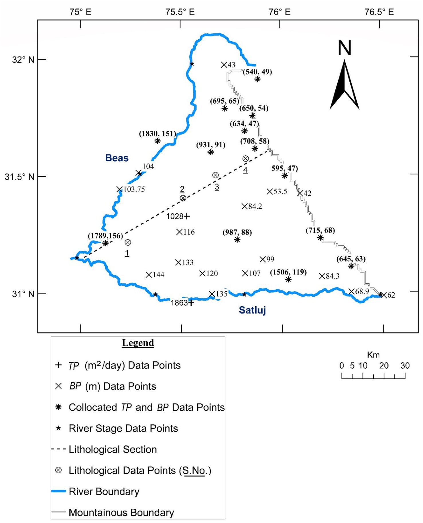
Figure 1. Index map of study area.

2.2.1 Study area

The study area spanning over 8,040 km² is inhabited by 5.26 million people (Economic and Statistical Organization, Government of Punjab, 2016). In terms of Land Use and Land Cover, approximately 80% of the geographical area in this region is covered by agricultural tracts. The detailed LULC analysis for the study area has been performed using ESA WorldCover (Zanaga et al., 2022) dataset in Google Earth Engine. ESA WorldCover provides a global LULC map for the year 2021 at a 10 m resolution. It provides 11 classes such as tree cover, shrubland, grassland, cropland, builtup area, bare lands, snow etc. Additional details for the same are presented in the Supplementary material. The underlying aquifer is composed of alluvium deposits consisting dominant sand strata with intermittent clay layers. Since the clay layers are nearly horizontal and spatially intermittent, the formation may be deemed to be a single horizontally isotropic unconfined aquifer. As per reported data, its saturated thickness varies from 42 m to 156 m and the transmissivity from 540 m²/day to 1830 m²/day from north-east to south-west (Central Ground Water Board, 2009; Singh et al., 2013). The area is served by southwest monsoon system with normal rainfall varying from 432 mm in southwest region to 759 mm in the north-east. A large part of annual rainfall (about 77%) occurs during monsoon season extending from June to October. The groundwater resource is primarily derived from the rainfall recharge with a relatively smaller contribution from two canal systems serving the area. The area is subjected to intensive groundwater development with about 95% of the withdrawals utilized for meeting irrigation demands. Contribution of the canal systems towards the irrigation demands is quite small. Rice and wheat are major crops of the area, with the former cultivated during monsoon season (locally referred as kharif season) and the latter in non-monsoon season (locally referred as rabi season). Consequent to the intensive agricultural groundwater development, especially for water intensive rice crop, the area is experiencing a watertable decline.

2.2.2 Data base

The envisaged cokriging requires sample T data (TP) and the sample B data (BP). Further, the proposed IP solution requires historical head fields and the corresponding withdrawals, recharge and boundary conditions. These data were gathered from several state and central government water resources agencies. Pumping test based TP data from 15 test sites (Figure 1) and well-log derived BP data from 58 bore sites were employed for the study. The available well logs were rather elementary displaying only “sand” and “clay” layers – broadly referring to permeable and non-permeable fractions, respectively. The saturated thickness values (BP) were arrived at by adding all the ‘sand’ thicknesses captured in the respective well logs. A few well log sites along with the corresponding values of saturated thickness are shown in Figure 1. Lithological profile for a representative section (refer Figure 1) along north-east direction is shown in Figure 2. Thirteen of the fifteen (TP) points have co-located (BP) points – leading to as many co-located (TP-BP) data points (Figure 1).

Figure 2

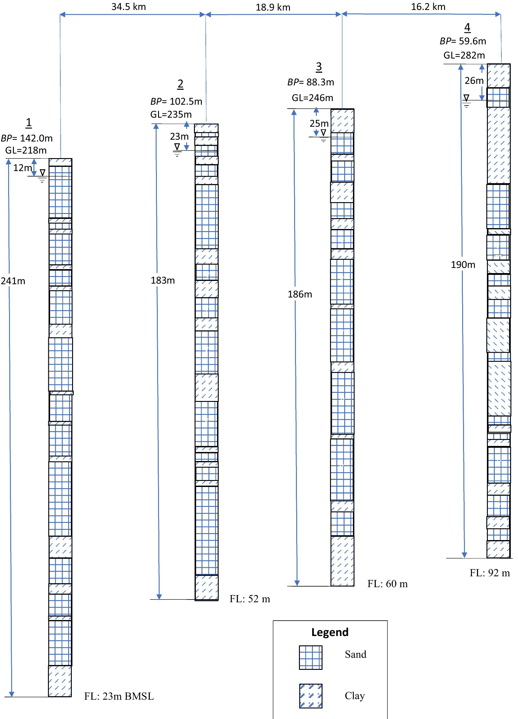
Figure 2. Lithological profile along the lithological section depicted in Figure 1.

Watertable data comprises observations from 91 wells at six discrete times over a period of three years extending from June-2014 to October-2016. These discrete times represent three pre-monsoon and two post-monsoon states. River stage data from six locations (three on Satluj, two on Beas and one at the confluence) at the same discrete times were employed for assigning the boundary conditions (Figure 1). The study area comprises 29 administrative blocks (Figure 3) and seasonal blockwise recharge/withdrawals and block-wise specific yield data were derived from published reports (CGWB, 2013).

Figure 3

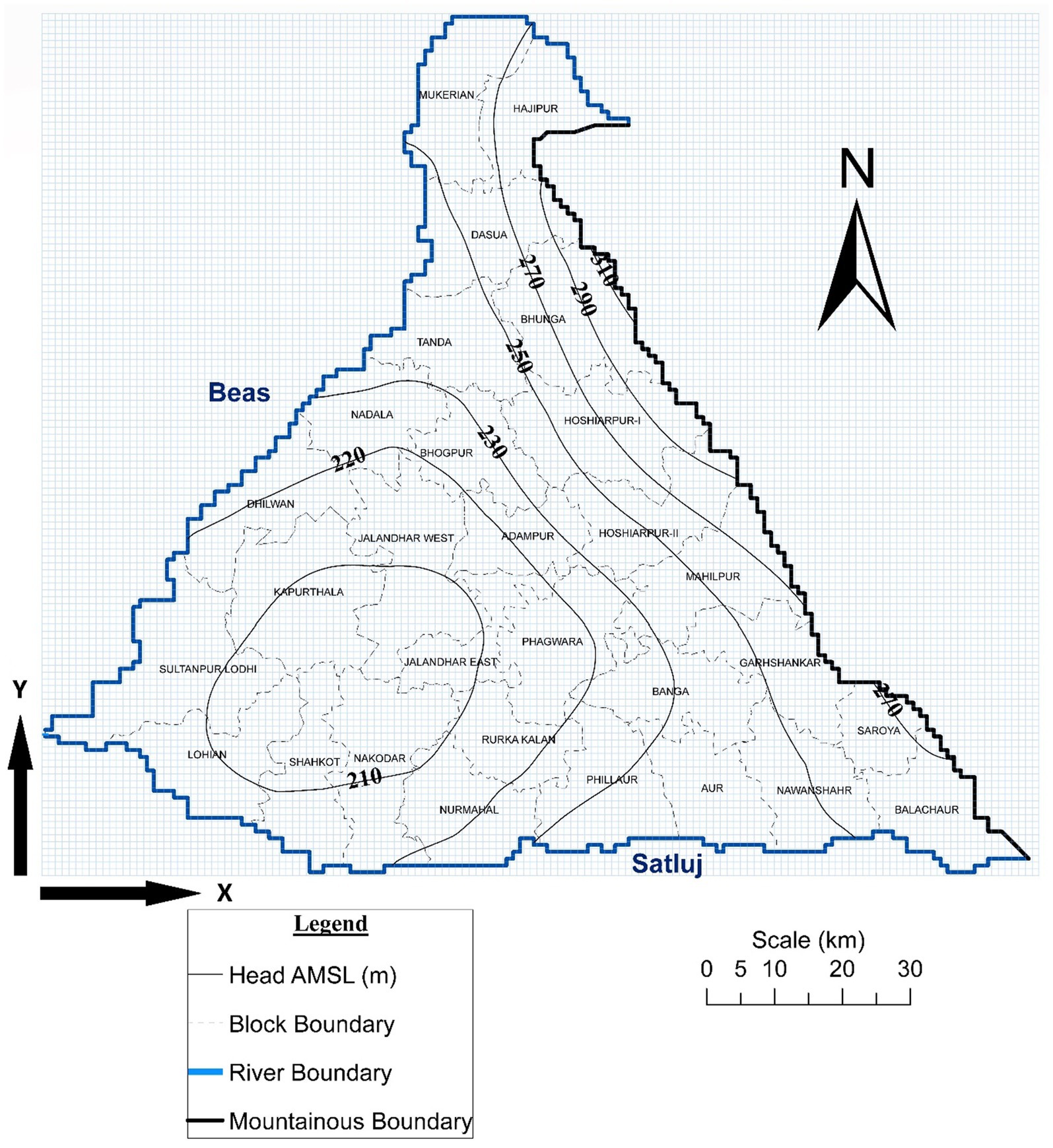
Figure 3. Block Boundaries and adopted initial condition.

2.2.3 Correlation between primary and secondary variables

The proposed cokriging model is an interpolator of the primary variable transmissivity (T) wherein the saturated thickness (B) is incorporated as the secondary variable. Although the correlation between variables T and B is depicted by the definition of T (i.e., T = KB), additional analyses were conducted to establish the necessary correlation between their respective sample values. As a first step, the co-located T and B data are plotted on linear scales (Figure 4). The scatter-points display a consistent rise of T as B increases – implying a positive correlation between the two. The points tend to fall between two enveloping straight lines (TP = 10.2BP, and TP = 13.5BP) – implying that K may be varying in the range (10.2 to13.5 m/day) in the region encompassed by the measurement points. Further, the correlation between T and B was established objectively by developing a cross- correlogram (Wackernagel, 2003) between T and B (Figure 5). This figure depicts the variation of the coefficient of correlation between T and B as a function of separation distance (h). It may be seen that a strong correlation (0.91) exists between co-located (h = 0) T and B values. The correlation vanishes asymptotically at a distance of about 35 km.

Figure 4

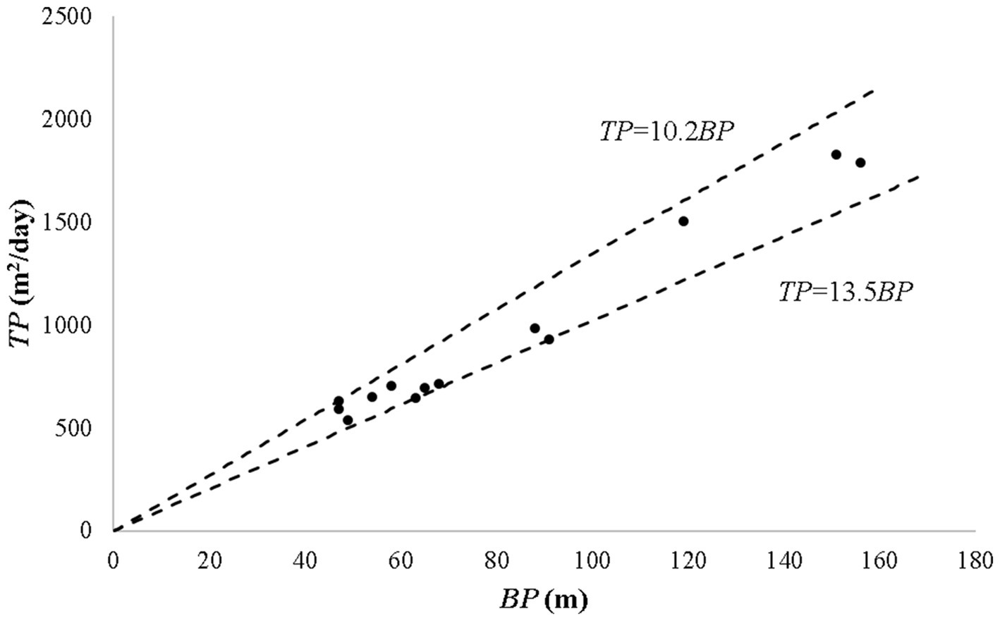
Figure 4. Variation in hydraulic conductivity.

Figure 5

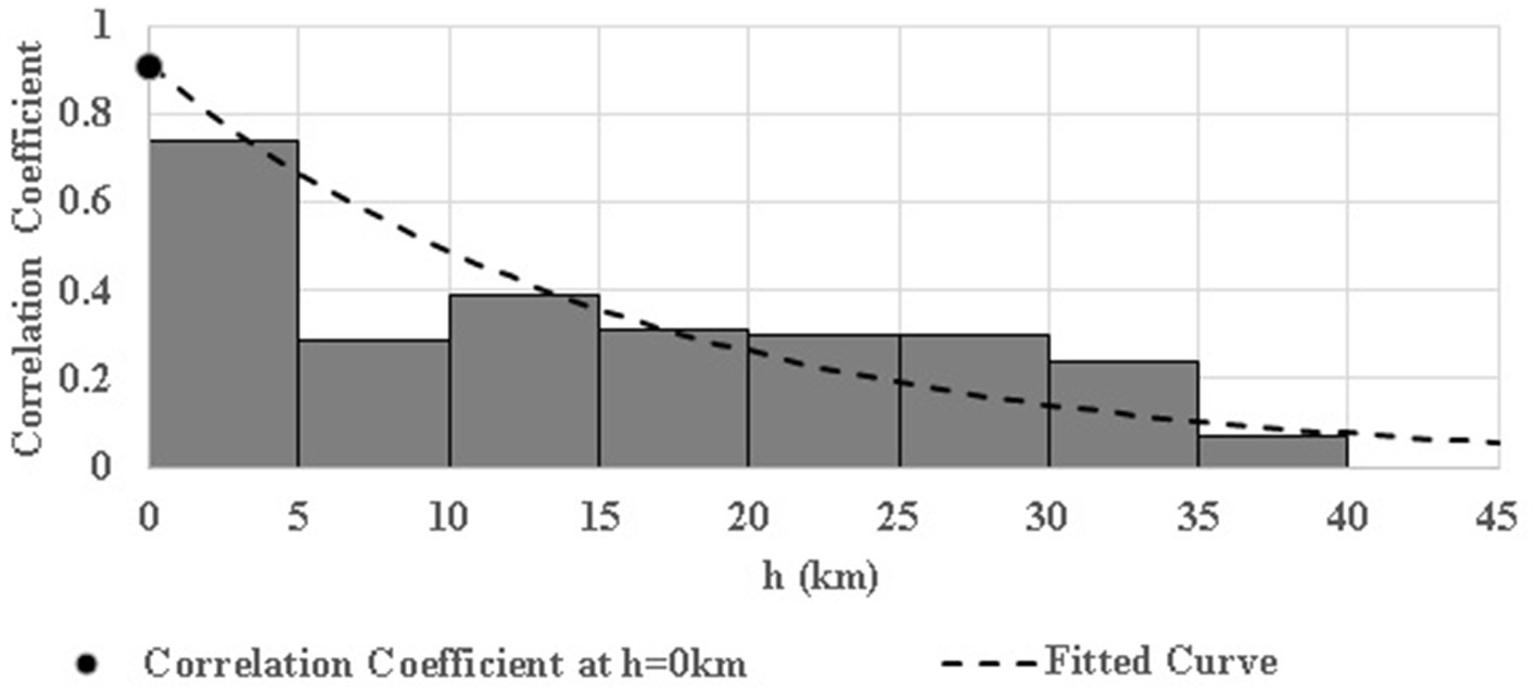
Figure 5. Cross-correlogram depicting variation in T-B cross-correlation coefficient with separating distance (h).

2.2.4 Detrending raw data

The available data (TP and BP) were detrended to fulfill the requirement of first order stationarity. Detrending has been performed by fitting least-squares 2-D plane equations in terms of X and Y (Figure 3), through TP(X,Y) and BP(X,Y) data points. Parameters of these planes viz., intercepts (T₀ and B₀ respectively) and gradients (trends) in x and y directions (I_XT and I_YT; I_XB and I_YB respectively) were estimated by regression analyses (Table 1). Finally, T and B data were detrended by simply subtracting the trend terms derived from the respective gradients.

Table 1

Table 1. Detrending parameters.

2.2.5 Generation of variograms/cross-variogram

These geostatistical attributes were generated employing the detrended data of TP_D (15 Nos.), BP_D (58 Nos.) and co-located (TP_D and BP_D) (13 Nos.). These data were utilized for developing experimental values of semivariances (${\hat{\gamma }}_{TT}$, ${\hat{\gamma }}_{BB}$ and ${\hat{\gamma }}_{TB}$) for an array of separating distances (h). These discrete point data of experimental variograms/cross-variogram are presented in Figures 6–8 respectively.

Figure 6

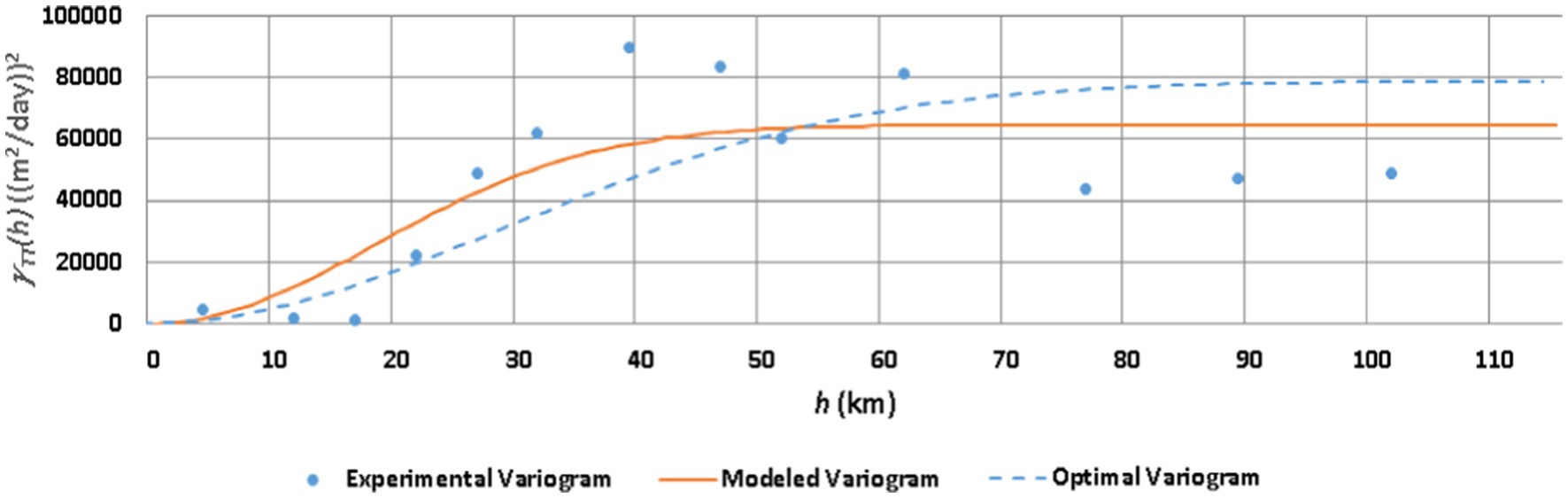
Figure 6. Experimental, modeled and IP-derived optimal T variograms.

Figure 7

Figure 7. Experimental and modeled B variograms.

Figure 8

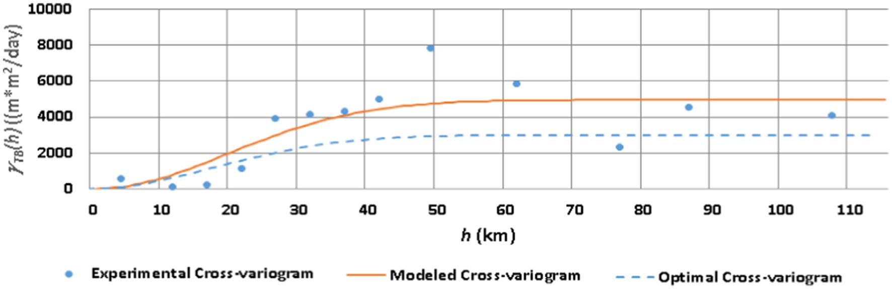
Figure 8. Experimental, modeled and IP-derived (Optimal) T-B cross-variograms.

Subsequently a theoretical model was fitted to each experimental variogram/cross-variogram by the least squares approach. The models were selected from an array of reported models (Kitanidis, 1997), on the basis of the “best” least-squares fit characterized by highest R². The reported models have two main characteristics viz. sill (${\sigma }^2$) and range (R). Whereas the sill is the limiting value of the semivariance as h tends to infinity, the range is the distance (h) at which the semivariance equals 95% of the sill. Gaussian and exponential variogram models (Kitanidis, 1997) were adopted for T and B, respectively. Gaussian cross-variogram model was adopted for T-B cross variogram Estimated geostatistical parameters for these models are presented in Table 2.

Table 2

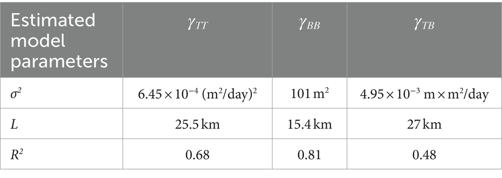
Table 2. Estimated parameters of models of variograms and cross-variogram.

As expected, R² for the model of B variogram is higher apparently on account of large number of sample (BP) points. On the other hand, the statistic values for the models of T variogram and T-B cross-variogram are lower owing to fewer sample points of (TP) and (TP-BP) data. This substantiates the need for refining the estimates of the model parameters of T variogram (termed as θ₁) and those of T-B cross-variogram (termed as θ₃). As such, the parameters (Ω) of the IP solution are defined as follows by Eq. 15.

$\begin{array}{ll}\mathrm{\Omega }=\left[\left({\sigma }_{\text{TT}}^2{,\mathrm{L}}_{\text{TT}},{\sigma }_{\text{TB}}^2{,\mathrm{L}}_{\text{TB}},\lambda \right)\right]& (15)\end{array}$

2.2.6 Interface of cokriging with IP

The cokriging model of T discussed in the preceding Sections was linked to a groundwater flow model of the study area for the estimation of the envisaged parameters (Ω) of the IP problem. The groundwater flow model employed in the present study is based upon a numerical solution of the differential equation presented in Eq. 16. governing two dimensional horizontal in an isotropic confined aquifer Eq. 16.

$\begin{array}{ll}\frac{\partial }{\partial X}\left(\mathrm{T}\frac{\partial h}{\partial X}\right)+\frac{\partial }{\partial Y}\left(\mathrm{T}\frac{\partial h}{\partial Y}\right)-\mathrm{W}=\left({\mathrm{S}}_{\mathrm{y}}\right)\frac{\partial h}{\partial t}& (16)\end{array}$

Where, T = isotropic transmissivity, h = head, X,Y = orthogonal cartesian coordinate, W = sink term, S_y = specific yield. Employing “current” values of (Ω), the T term appearing in above equation is cokriged as per Eqs. 7, 8 using the sample points (TP and BP) falling within the respective search radius (=7/4L_TT). This confined flow equation incorporating isotropic transmissivity as a time-averaged flow parameter has been invoked for modeling the unconfined flow assuming (i) horizontal isotropy, (ii) small enough temporal fluctuation of h and (iii) flat spatial gradients honoring Dupuit-Forchheimer assumptions. The adopted flow equation was solved to simulate the head fields at advancing discrete times using IADI based finite difference method. The flow model was externally linked to an optimizer based upon SUMT algorithm (Fiacco and McCormick, 1990) to facilitate the estimation of (Ω).

Adopting a spatial discretization of 1,000 m, a finite difference grid (Figure 3) comprising 8,350 active nodes and 418 boundary nodes was superposed over the study area. Recalling that the head data are available at six discrete times (over a period of three years extending from June-2014 to October-2016), the June-2014 head field was treated as the initial condition (Figure 3). Head fields at the following five discrete times (until October 2016) were simulated adopting a time interval of 15 days. The boundary conditions at the river boundary nodes were assigned as per the available river stage data. Neuman boundary condition was assigned along the mountainous boundary. The necessary flux rate was derived from the prevailing hydraulic gradients. The forcing function vector (W) was derived from the available recharge/withdrawal data.

The vector of poorly known/unknown parameters (Ω) was estimated by minimizing the mismatch between the observed and the simulated head fields of October 2016. Accordingly, the IP is defined as the following optimization problem (Eq. 17).

$\begin{array}{l}\mathit{\text{Minimize}}\mathrm{Z}={\displaystyle {\sum }_{\mathrm{i}=1}^{\text{na}}{\left({\hat{\mathrm{h}}}_{\mathrm{i}}-{\mathrm{h}}_{\mathrm{i}}\right)}^2\text{wrt}.\text{Five decision variables}}\\ \left[\mathrm{\Omega }=\left({\sigma }_{\text{TT}}^2{,\mathrm{L}}_{\text{TT}},{\sigma }_{\text{TB}}^2{,\mathrm{L}}_{\text{TB}},\lambda \right)\right]\end{array}\text{ (17)}$

Where, na = number of active nodes, ${\hat{h}}_i$= observed head at ith active node at October 2016, and $h_i$=simulated head at ith active node at October 2016. Constraints were assigned to ensure non-negativity of all the five variables. Further, the fifth decision variable (λ) was contrained as in Eq. 18.

$\begin{array}{ll}0\le \lambda \le 1& (18)\end{array}$

3 Results

Recalling that the poorly known/unknown cokriging parameters (Ω) are treated as the IP parameters (and hence decision variables of the proposed optimization problem), their initial and the optimized values along with the corresponding objective function values are presented in Table 3. It may be seen that the parameters undergo a substantial variation leading to a reduction of the objective function from 1954 m² to 1,609 m². The corresponding cokriged-IP T field is presented in Figure 9.

Table 3

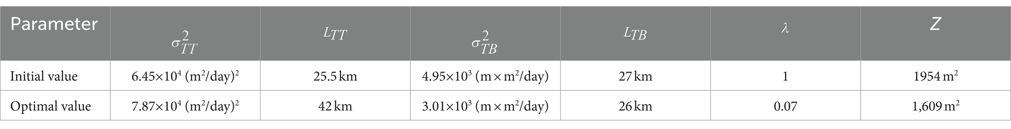
Table 3. Initial and optimal geostatistical parameters.

Figure 9

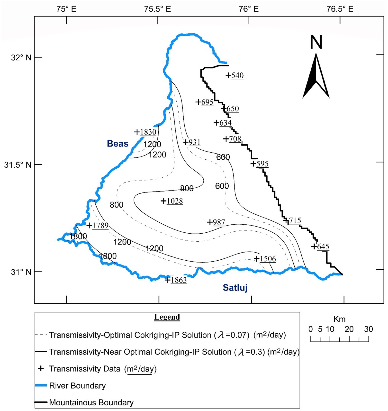
Figure 9. Optimal and pareto-front (near-optimal) transmissivity fields.

It may be noted that the resultant optimal value of $\lambda$ is quite low (0.07)—apparently on account of relatively sparse and some-what clustered T data. This implies that the interpolation of T has been largely governed by BP data with a relatively smaller role of TP data. This in turn has led to large mismatch between the interpolated and sampled T values at the sampling points (Figure 9). Although this kind of mismatch is quite common in practical calibrations (Davis et al., 2015), attempt was made to control it as much as possible to enhance plausibility (RamaRao et al., 1995) of the cokriged T field without significantly compromising upon the optimality of Z. This was done enforcing representing T mismatch as expressed in Eq. 19.

$\begin{array}{ll}\mathit{\text{Minimize}}\mathrm{Z}1=\frac{1}{\mathrm{n}}{\displaystyle \sum _{\mathrm{n}}}\left|\frac{{\mathrm{T}}_{\text{oi}}-{\text{TP}}_{\mathrm{i}}}{{\text{TP}}_{\mathrm{i}}}\right|\times 100& (19)\end{array}$

Where, TP_i, T_oi = measured and IP-cokriged transmissivity at ith sampling location, respectively, and n = number of sampled TP data.

The multi-objective minimization of Z and Z₁ was conducted by applying the principle of Pareto front optimization (Goodarzi et al., 2014; Rao, 2019) which in the present context would imply minimizing Z without undue degradation of Z₁. A Pareto front depicting variation of Z and Z₁ at increasing λ values is presented in Figure 10. The front clearly shows that (λ = 0.07) though an optimal solution in context of Z compromises on minimization of Z₁. As λ increases from 0.07 to 0.3, increase of Z is minimal (1,609 to 1,631 m²) with a notable decrease in Z₁. However, as λ increases beyond 0.3, Z increases rapidly with a pronouncedly larger gradient. Thus, (λ = 0.3) may be deemed to be the Pareto front optimal solution since around it there is no way of decreasing Z without increasing Z₁ sharply. As such, the optimal value of the decision variable $\lambda$ was modified to 0.3. Incidentally this value of λ also nearly equals the ratio of B and T data. The corresponding modified T field is superposed over the initial T ($\lambda$ = 0.07) field (Figure 9). The former field though still displaying departure from the sampled T values, honors them more closely as compared to the latter one. The departure is more pronounced in central-south-western region wherein T data are sparse but B data are well available.

Figure 10

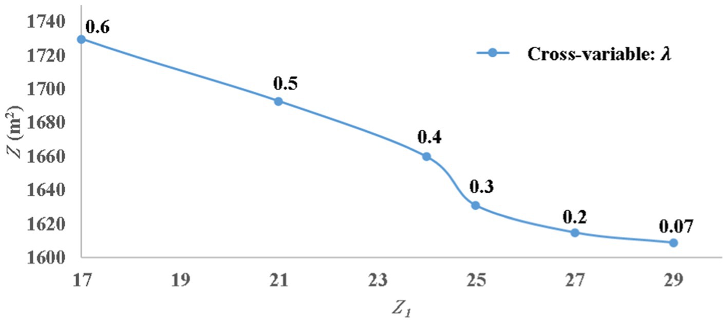
Figure 10. Computed pareto front.

The contours of the simulated heads corresponding to the modified T field at the target time (October 2016) are presented in the Supplementary Figure S2. However, since the residuals (${\hat{h}}_i-h_i$) are not discernible in these contours because of the scale effect, the spatial distribution of the nodal residuals is depicted explicitly in Supplementary Figure S3. The variograms and cross-variogram derived from the initial and optimal parameters, along with the experimental points, are presented in Figures 6–8.

4 Discussion of results

Results presented in Table 3 reveal that parameters L_TT and λ change significantly as the cokriging interpolator is joined with the envisaged IP solution. The assigned initial value (25.5 km) of L_TT emanates from regression of limited number of experimental points with rather low R² (0.68). The optimized value (42 km) is significantly higher implying a substantially enhanced range (R = 7/4L_TT). This indicates that the spatial auto-correlation of T extends over much longer distance than what is revealed by the limited TP data. The distribution parameter (λ) is near- optimized as 0.30 – implying a larger weight to the BP data as compared to the TP data. This weighing proportion seems to be reasonable in view of the relative sparseness of TP data. The transmissivity field emanating from the proposed approach has resulted in much improved reproduction of the observed head field – evidenced by improved Z (Table 3).

For gaining additional insight, hydraulic conductivity (K) field was generated (Figure 11) by dividing the IP-cokriged T field by the kriged B field (Figure 12). The K field displays a variation from 7 to 15 m/day which extends beyond the range of 10.2 to 13.5 m/day depicted in Figure 4. Recalling that Figure 4 is derived from the limited co-located T-B data, the expansion of the K range is accomplished through IP-cokriging assisted interplay between the head and (T, B) data including the ones among the latter that are not co-located. This facilitates production of more realistic K and T fields. For example, this has permitted capture of hydrogeologically consistent low K in the interior zone and high K near river Satluj (shown as sites A and B in Figure 11) in spite of absence of any co-located T-B data there.

Figure 11

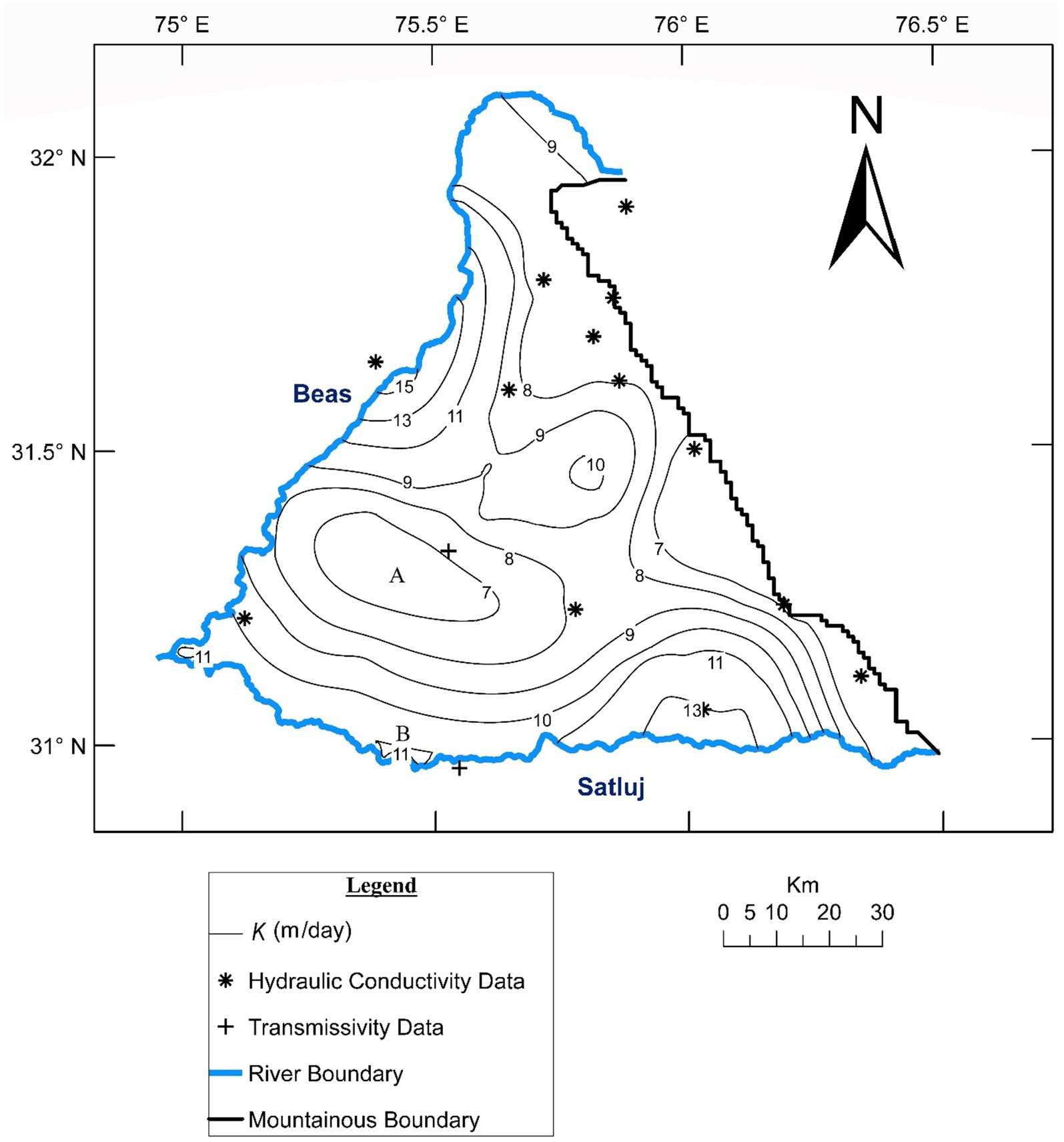
Figure 11. K field emanating from proposed model and B field (refer Figure 12).

Figure 12

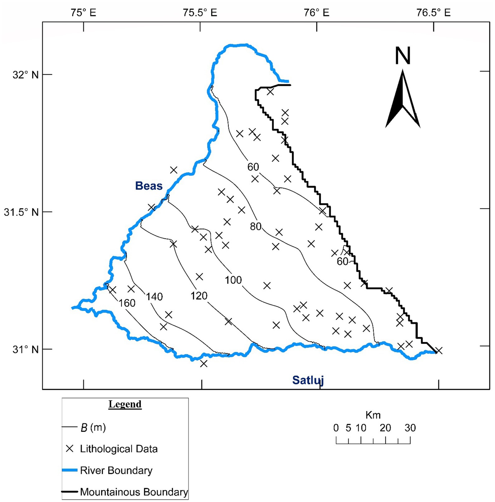
Figure 12. B Field obtained by kriging the BP data.

5 Validation of T field

It may be recalled that while solving the envisaged IP, the head field of the June 2014 was treated as the initial condition and the fields of the following five discrete times (until October 2016) were simulated. However, the head based IP solution was defined in terms of the mismatch between the observed and the simulated fields of October 2016 only—not using the observed head fields of four intervening discrete times. As such, October 2016 and the four preceding simulation times are henceforth termed as target and non-target times, respectively. Validity of the optimal parameter estimates (and hence of the resulting T field) has been linked to the reproduction of the observed fields at the non-target times.

Values of the mismatch parameter Z (Eq. 13) at the target as well as non-target times are presented in Table 4. It may be seen that Z values at the non-target times are not conspicuously higher than the optimized value (1,631 m²) corresponding to the target time. The time series of the observed and simulated heads at four typical locations OW1, OW2, OW3, OW4 (Supplementary Figure S3) are presented in Supplementary Figure S4. Again, the observed head time series are quite well reproduced at the target as well as non-target times. These inferences validate the parameter estimation and the consequent transmissivity field.

Table 4

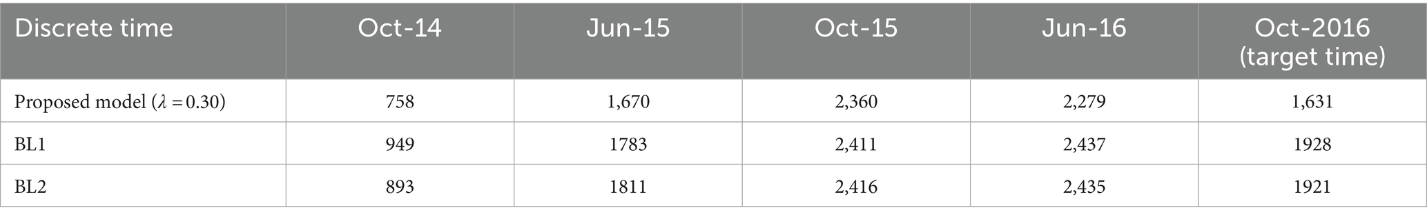
Table 4. Z (m²) at target and non-target times.

6 Baseline studies

The proposed model for generation of T field invokes a cokriging-IP based solution. However, there could be relatively simpler/practice-oriented modeling options viz. (i) kriging of TP and (ii) kriging of K(=TP/BP) and BP, and multiplying the two to obtain T field. Performance metrics of these baseline options (termed, respectively, as BL1and BL2) were compared with those of the proposed model. As a first step towards the comparison, an alternative T field was generated using the baseline model under reckoning. This was subsequently employed for simulating the head fields at five discrete times viz. four non-target times and the target time (October 2016) referred to in the Validation Section.

The transmissivity fields emanating from the proposed model, BL1 and BL2 are presented in Figure 13. Corresponding values of the mismatch parameter (Z) were derived from these head fields (Table 4). It may be seen that compared to BL1 and BL2, the proposed model yields significantly reduced Z values at all discrete times including the non-target ones. This clearly demonstrates superiority of the proposed model over BL1 and BL2. It may also be seen that in spite of using additional data, BL2 does not lead to significantly lower Z values in comparison to those from BL1. It may be seen that BL1 and BL2 lead to almost similar transmissivity fields (Figure 13). It may be inferred that independent usage of T and B data does not provide any value addition over using only T data. It is the synergic and simultaneous deployment of both T and B data that improves the credibility of resulting T fields.

Figure 13

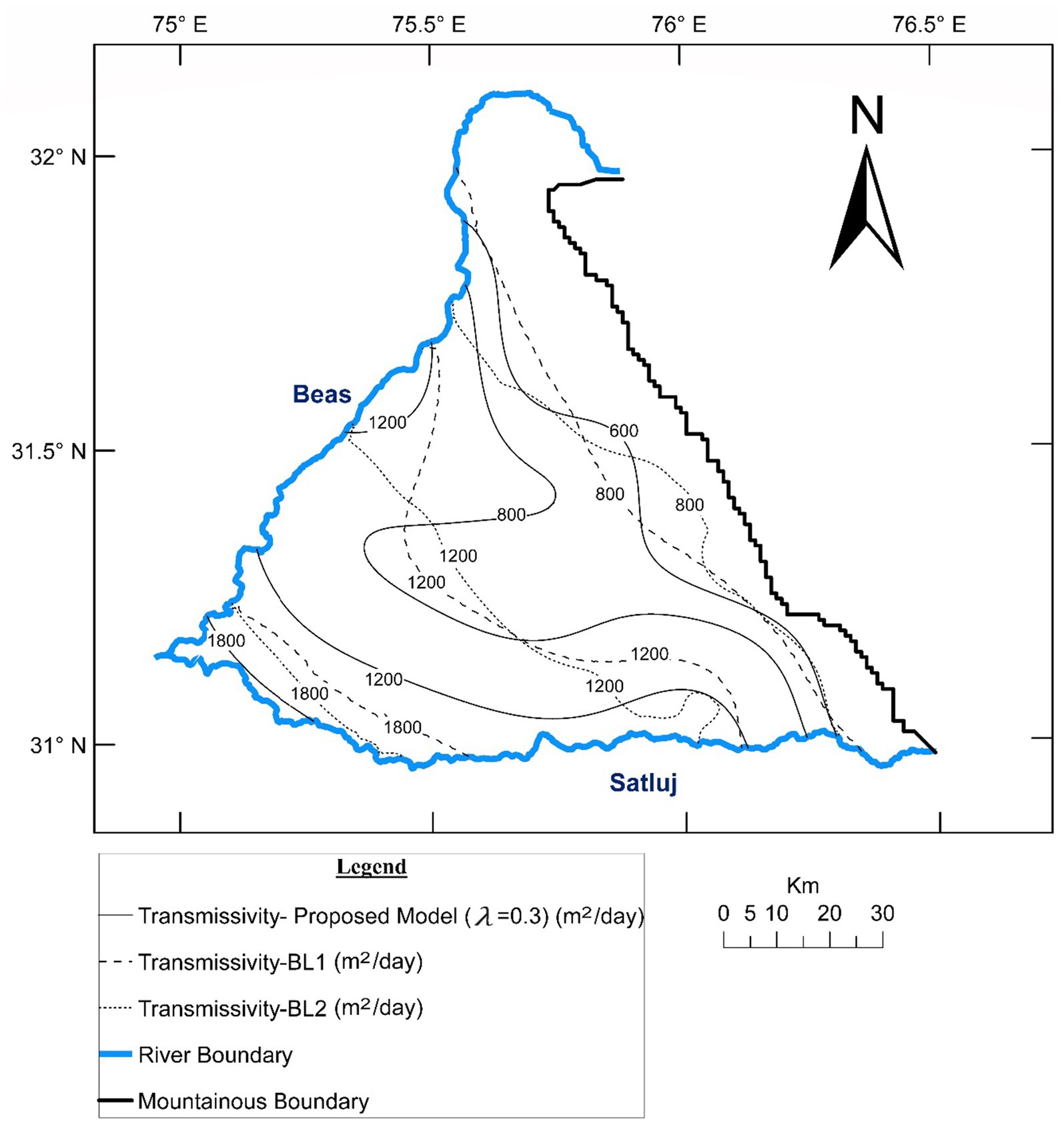
Figure 13. Transmissivity fields (proposed model, BL1 and BL2).

The generated T field has also been informally validated by invoking the corresponding K field (Refer Figure 12) that was computed by dividing the proposed T field by B field. The field displays K variation from 7 to 15 m/day which falls in the broad range for sands (Domenico and Schwartz, 1990). Recalling that B represents cumulative ‘sand’ thickness, this may be deemed to be an elementary validation of the generated T field.

7 Conclusion

The proposed IP-joined cokriging interpolator permits credible generation of transmissivity fields even when the primary T data are sparse. The data sparseness is overcome by simultaneously invoking data of other T-correlated secondary variable B, and moderating the unknown/poorly known cokriging parameters. In the present study, combination of sparse T data with abundantly available saturated thickness values has been shown to be work well. However, recourse can be taken to other secondary variables like formation loss parameter (derived from step-drawdown tests), geophysical resistivity etc. The prevalent practice of IP solution is generally aimed at moderating the available T data or estimating T values at stipulated un-gauged locations. However, as has been demonstrated in this study, the IP solution can also be used for modification of poorly known geostatistical parameters of cokriging, apart from estimating the unknown ones. The study reveals that adopting IP- joined cokriging in place of kriging may lead to a substantial improvement in the reproduction of the observed head fields. This in turn may imply enhanced head prediction capability of the generated transmissivity fields.

Data availability statement

The raw data supporting the conclusions of this article will be made available by the authors, without undue reservation.

Author contributions

AK: Conceptualization, Data curation, Formal analysis, Investigation, Methodology, Resources, Software, Validation, Visualization, Writing – original draft, Writing – review & editing. DK: Conceptualization, Funding acquisition, Investigation, Methodology, Project administration, Resources, Software, Supervision, Validation, Visualization, Writing – original draft, Writing – review & editing, Formal analysis.

Funding

The author(s) declare that no financial support was received for the research, authorship, and/or publication of this article.

Acknowledgments

The data used in the present study was gathered from Water Resources Organization, Punjab; Department of Agriculture, Punjab; and Central Groundwater Board, Chandigarh. Authors are thankful to Chief Engineer K.S. Takshi, Mr. Neeraj Pandit and Mr. Tejdeep Singh from these organizations for their help and meaningful discussions. Authors are also thankful to Indian Institute of technology Ropar for providing the facilities to perform this research.

Conflict of interest

The authors declare that the research was conducted in the absence of any commercial or financial relationships that could be construed as a potential conflict of interest.

Publisher’s note

All claims expressed in this article are solely those of the authors and do not necessarily represent those of their affiliated organizations, or those of the publisher, the editors and the reviewers. Any product that may be evaluated in this article, or claim that may be made by its manufacturer, is not guaranteed or endorsed by the publisher.

Supplementary material

The Supplementary material for this article can be found online at: https://www.frontiersin.org/articles/10.3389/frwa.2024.1380761/full#supplementary-material

Abbreviations

BL, baseline; ESA, European space agency; IADI, iterative alternating direction implicit; IP, inverse problem; LSO, linked simulation optimization; LULC, land use land cover; SHD, secondary hydrogeological data; SUMT, sequentially unconstrained minimization technique; SC, specific capacity; T, transmissivity (primary variable); OW, observation well.

References

Aboufirassi, M., and Mariño, M. A. (1984). Cokriging of aquifer transmissivities from field measurements of transmissivity and specific capacity. J. Int. Assoc. Math. Geol. 16, 19–35. doi: 10.1007/BF01036238

Crossref Full Text | Google Scholar

Adhikary, S. K., Muttil, N., and Yilmaz, A. G. (2017). Cokriging for enhanced spatial interpolation of rainfall in two Australian catchments. Hydrol. Process. 31, 2143–2161. doi: 10.1002/hyp.11163

Crossref Full Text | Google Scholar

Ahmed, S., and de Marsily, G. (1987). Comparison of geostatistical methods for estimating transmissivity using data on transmissivity and specific capacity. Water Resour. Res. 23, 1717–1737. doi: 10.1029/WR023i009p01717

Crossref Full Text | Google Scholar

Ahmed, S., de Marsily, G., and Talbot, A. (1988). Combined use of hydraulic and electrical properties of an aquifer in a geostatistical estimation of transmissivity. Groundwater 26, 78–86. doi: 10.1111/j.1745-6584.1988.tb00370.x

Crossref Full Text | Google Scholar

Alam, F., and Umar, R. (2013). Groundwater flow modelling of Hindon-Yamuna interfluve region, western Uttar Pradesh. J. Geol. Soc. India 82, 80–90. doi: 10.1007/s12594-013-0113-8

Crossref Full Text | Google Scholar

Anderson, M. P., Woessner, W. W., and Hunt, R. J. (2015). Applied groundwater modeling: Simulation of flow and advective transport. Amsterdam, Netherlander: Academic press.

Google Scholar

Bailey, R. T., Abbas, S., Arnold, J., White, M., Gao, J., and Čerkasova, N. (2023). Augmenting the national agroecosystem model with physically based spatially distributed groundwater modeling. Environ. Model Softw. 160:105589. doi: 10.1016/j.envsoft.2022.105589

Crossref Full Text | Google Scholar

Belkhiri, L., Tiri, A., and Mouni, L. (2020). Spatial distribution of the groundwater quality using kriging and co-kriging interpolations. Groundw. Sustain. Dev. 11:100473. doi: 10.1016/j.gsd.2020.100473

Crossref Full Text | Google Scholar

Bhattacharjya, R. K., and Datta, B. (2005). Optimal management of coastal aquifers using linked simulation optimization approach. Water Resour. Manag. 19, 295–320. doi: 10.1007/s11269-005-3180-9

Crossref Full Text | Google Scholar

Cardiff, M., and Barrash, W. (2011). 3-D transient hydraulic tomography in unconfined aquifers with fast drainage response. Water Resour. Res. 47:367. doi: 10.1029/2010WR010367

Crossref Full Text | Google Scholar

Central Ground Water Board (2009). Report of the working group on methodology for assessment of development potential of deeper aquifers. Faridabad: Central Ground Water Board, pp.26–27.

Google Scholar

Certes, C., and de Marsily, G. (1991). Application of the pilot point method to the identification of aquifer transmissivities. Adv. Water Resour. 14, 284–300. doi: 10.1016/0309-1708(91)90040-U

Crossref Full Text | Google Scholar

Chapra, S. C., and Canale, R. P., (2010). Numerical methods for engineers. Boston: McGraw-Hill Higher Education. ISBN: 978-0073401065

Google Scholar

Christelis, V., Kopsiaftis, G., Regis, R. G., and Mantoglou, A. (2023). An adaptive multi-fidelity optimization framework based on co-kriging surrogate models and stochastic sampling with application to coastal aquifer management. Adv. Water Resour. 180:104537. doi: 10.1016/j.advwatres.2023.104537

Crossref Full Text | Google Scholar

Cui, T., Pagendam, D., and Gilfedder, M. (2021). Gaussian process machine learning and kriging for groundwater salinity interpolation. Environ. Model Softw. 144:105170. doi: 10.1016/j.envsoft.2021.105170

Crossref Full Text | Google Scholar

CGWB, (2013). Dynamic Groundwater Resources of Punjab. Central Groundwater Board and Water Resources and Environment Directorate of Punjab. Chandigarh.

Google Scholar

Davis, K. W., Putnam, L. D., and LaBelle, A. R. (2015). Conceptual and numerical models of groundwater flow in the Ogallala and Arikaree aquifers, pine ridge Indian reservation area, South Dakota, water years 1980-2009 (no. 2014-5241). Reston, Virginia, USA: US Geological Survey.

Google Scholar

Dickson, N. E., Comte, J. C., Koussoube, Y., Ofterdinger, U. S., and Vouillamoz, J. M. (2019). Analysis and numerical modelling of large-scale controls on aquifer structure and hydrogeological properties in the African basin (Benin, West Africa). Geol. Soc. Lond., Spec. Publ. 479, 81–100. doi: 10.1144/SP479.2

Crossref Full Text | Google Scholar

Domenico, P. A., and Schwartz, F. W., (1990). Physical and chemical hydrogeology, John Wiley & Sons, New York, 824.

Google Scholar

Economic and Statistical Organization, Government of Punjab, (2016). District Domestic Product Of Punjab (2011-12 To 2015-16). [online] EPOSB. Available at: https://www.esopb.gov.in/static/PDF/Publications/State-Income/DDP-2011-12TO2015-16.pdf (Accessed 15 May 2020).

Google Scholar

Escriva-Bou, A., Hui, R., Maples, S., Medellín-Azuara, J., Harter, T., and Lund, J. R. (2020). Planning for groundwater sustainability accounting for uncertainty and costs: an application to California’s Central Valley. J. Environ. Manag. 264:110426. doi: 10.1016/j.jenvman.2020.110426

PubMed Abstract | Crossref Full Text | Google Scholar

Fiacco, A. V., and McCormick, G. P. (1990). Nonlinear programming: sequential unconstrained minimization techniques. Soc. Indus. Appl. Math. 12, 593–594. doi: 10.1137/1012119

Crossref Full Text | Google Scholar

Gannett, M. W., Wagner, B. J., and Lite, K. E. (2012). Groundwater simulation and management models for the upper Klamath basin, Oregon and California. Reston, Virginia, USA: US Department of the Interior, US Geological Survey.

Google Scholar

Ghosh, S., and Kashyap, D. (2012). Kernel function model for planning of agricultural groundwater development. J. Water Resour. Plan. Manag. 138, 277–286. doi: 10.1061/(ASCE)WR.1943-5452.0000178

Crossref Full Text | Google Scholar

Goodarzi, E., Ziaei, M., and Hosseinipour, E. Z., (2014). Introduction to optimization analysis in hydrosystem engineering. New York, NY: Springer International Publishing.

Google Scholar

Hoeksema, R. J., and Kitanidis, P. K. (1985). Analysis of the spatial structure of properties of selected aquifers. Water Resour. Res. 21, 563–572. doi: 10.1029/WR021i004p00563

Crossref Full Text | Google Scholar

Isaaks, E. H., and Srivastava, R. M. (1989). An Introduction to Applied Geostatistics. Oxford University Press, New York, 413.

Google Scholar

Izady, A., Joodavi, A., Ansarian, M., Shafiei, M., Majidi, M., Davary, K., et al. (2022). A scenario-based coupled SWAT-MODFLOW decision support system for advanced water resource management. J. Hydroinf. 24, 56–77. doi: 10.2166/hydro.2021.081

Crossref Full Text | Google Scholar

Jazaei, F., Waldron, B., Schoefernacker, S., and Larsen, D. (2019). Application of numerical tools to investigate a leaky aquitard beneath urban well fields. Water 11:5. doi: 10.3390/w11010005

Crossref Full Text | Google Scholar

Júnez-Ferreira, H. E., Hernández-Hernández, M. A., Herrera, G. S., González-Trinidad, J., Cappello, C., Maggio, S., et al. (2023). Assessment of changes in regional groundwater levels through spatio-temporal kriging: application to the southern basin of Mexico aquifer system. Hydrogeol. J. 31, 1405–1423. doi: 10.1007/s10040-023-02681-y

Crossref Full Text | Google Scholar

Kapoor, A., and Kashyap, D. (2021). Parameterization of pilot point methodology for supplementing sparse transmissivity data. Water 13:2082. doi: 10.3390/w13152082

Crossref Full Text | Google Scholar

Kavusi, M., Khashei Siuki, A., and Dastourani, M. (2020). Optimal design of groundwater monitoring network using the combined election-kriging method. Water Resour. Manag. 34, 2503–2516. doi: 10.1007/s11269-020-02568-7

Crossref Full Text | Google Scholar

Kitanidis, P. K. (1997). Introduction to geostatistics: Applications in hydrogeology. Cambridge, United Kingdom: Cambridge University Press.

Google Scholar

Kitanidis, P. K., and Vomvoris, E. G. (1983). A geostatistical approach to the inverse problem in groundwater modeling (steady state) and one-dimensional simulations. Water Resour. Res. 19, 677–690. doi: 10.1029/WR019i003p00677

Crossref Full Text | Google Scholar

LaVenue, A. M., and Pickens, J. F. (1992). Application of a coupled adjoint sensitivity and kriging approach to calibrate a groundwater flow model. Water Resour. Res. 28, 1543–1569. doi: 10.1029/92WR00208

Crossref Full Text | Google Scholar

Maliva, R. G., Manahan, W. S., and Missimer, T. M. (2021). Climate change and water supply: governance and adaptation planning in Florida. Water Policy 23, 521–536. doi: 10.2166/wp.2021.140

Crossref Full Text | Google Scholar

Mamo, S., Birhanu, B., Ayenew, T., and Taye, G. (2021). Three-dimensional groundwater flow modeling to assess the impacts of the increase in abstraction and recharge reduction on the groundwater, groundwater availability and groundwater-surface waters interaction: a case of the rib catchment in the Lake Tana sub-basin of the upper Blue Nile River, Ethiopia. J. Hydrol. Reg. Stud. 35:100831. doi: 10.1016/j.ejrh.2021.100831

Crossref Full Text | Google Scholar

Marino, M. A. (2001). “Conjunctive management of surface water and groundwater” in Regional management of water resources Journal of the International Association for Mathematical Geology, vol. 268, 165–173.

Google Scholar

McKinney, D. C., and Lin, M. D. (1994). Genetic algorithm solution of groundwater management models. Water Resour. Res. 30, 1897–1906. doi: 10.1029/94WR00554

Crossref Full Text | Google Scholar

Miller, N. L., Dale, L. L., Brush, C. F., Vicuna, S. D., Kadir, T. N., Dogrul, E. C., et al. (2009). Drought resilience of the California Central Valley surface-ground-water-conveyance system 1. J. Am. Water Res. Ass. 45, 857–866. doi: 10.1111/j.1752-1688.2009.00329.x

Crossref Full Text | Google Scholar

Olea, R. A. (2018). A practical primer on geostatistics (no. 2009−1103). New York, USA: Reston, Virginia, USA: US Geological Survey.

Google Scholar

Oliver, M. A., and Webster, R. (2015). Basic steps in Geostatistics: the variogram and kriging, springer briefs in agriculture. 2211–808X, vol. 1 Springer.

Google Scholar

Panagiotou, C. F., Kyriakidis, P., and Tziritis, E. (2022). Application of geostatistical methods to groundwater salinization problems: a review. J. Hydrol. 615:128566. doi: 10.1016/j.jhydrol.2022.128566

Crossref Full Text | Google Scholar

Rai, P. K., and Tripathi, S. (2019). Gaussian process for estimating parameters of partial differential equations and its application to the Richards equation. Stoch. Env. Res. Risk A. 33, 1629–1649. doi: 10.1007/s00477-019-01709-8

Crossref Full Text | Google Scholar

RamaRao, B. S., LaVenue, A. M., De Marsily, G., and Marietta, M. G. (1995). Pilot point methodology for automated calibration of an ensemble of conditionally simulated transmissivity fields: 1. Theory and computational experiments. Water Resour. Res. 31, 475–493. doi: 10.1029/94WR02258

Crossref Full Text | Google Scholar

Rao, S. S. (2019). Engineering optimization: theory and practice. Hoboken, New Jersey: John Wiley & Sons.

Google Scholar

Senoro, D. B., de Jesus, K. L. M., Mendoza, L. C., Apostol, E. M. D., Escalona, K. S., and Chan, E. B. (2021). Groundwater quality monitoring using in-situ measurements and hybrid machine learning with empirical Bayesian kriging interpolation method. Appl. Sci. 12:132. doi: 10.3390/app12010132

Crossref Full Text | Google Scholar

Singh, A., Panda, S. N., Kumar, K. S., and Sharma, C. S. (2013). Artificial groundwater recharge zones mapping using remote sensing and GIS: a case study in Indian Punjab. Environ. Manag. 52, 61–71. doi: 10.1007/s00267-013-0101-1

PubMed Abstract | Crossref Full Text | Google Scholar

Singh, A., Panda, S. N., Saxena, C. K., Verma, C. L., Uzokwe, V. N., Krause, P., et al. (2016). Optimization modeling for conjunctive use planning of surface water and groundwater for irrigation. J. Irrig. Drain. Eng. 142:04015060. doi: 10.1061/(ASCE)IR.1943-4774.0000977

Crossref Full Text | Google Scholar

Wackernagel, H. (2003). Multivariate Geostatistics. Berlin, Heidelberg: Springer Berlin Heidelberg.

Google Scholar

Yao, L., Huo, Z., Feng, S., Mao, X., Kang, S., Chen, J., et al. (2014). Evaluation of spatial interpolation methods for groundwater level in an arid inland oasis, Northwest China. Environ. Earth Sci. 71, 1911–1924. doi: 10.1007/s12665-013-2595-5

Crossref Full Text | Google Scholar

Yeh, W. W. (2015). Optimization methods for groundwater modeling and management. Hydrogeol. J. 23, 1051–1065. doi: 10.1007/s10040-015-1260-3

Crossref Full Text | Google Scholar

Yeh, T. C. J., Gutjahr, A. L., and Jin, M. (1995). An iterative cokriging-like technique for ground-water flow modeling. Groundwater 33, 33–41. doi: 10.1111/j.1745-6584.1995.tb00260.x

Crossref Full Text | Google Scholar

Yoon, Y. S., and Yeh, W. G. (1976). Parameter identification in an inhomogeneous medium with the finite-element method. Soc. Pet. Eng. J. 16, 217–226. doi: 10.2118/5524-PA

Crossref Full Text | Google Scholar

Zanaga, D., Van De Kerchove, R., Daems, D., De Keersmaecker, W., Brockmann, C., Kirches, G., et al., (2022). ESA WorldCover 10 m 2021 v200. Zenodo.

Google Scholar

Zawadzki, J., Fabijańczyk, P., and Treichel, W. (2021). Monitoring of groundwater quality with cokriging of geochemical and geoelectrical measurements. Multidiscip. Aspects Prod. Eng. 4, 97–106. doi: 10.2478/mape-2021-0009

Crossref Full Text | Google Scholar

Zeinali, M., Azari, A., and Heidari, M. M. (2020). Multiobjective optimization for water resource management in low-flow areas based on a coupled surface water–groundwater model. J. Water Resour. Plan. Manag. 146:04020020. doi: 10.1061/(ASCE)WR.1943-5452.000118

Crossref Full Text | Google Scholar

Zhao, Z., Zhang, L., and Bi, E. (2022). Spatial interpolation of highly skewed data of the Junggar Basin phreatic groundwater through the multi-scale cokriging model. Earth Sci. Inf. 15, 1737–1748. doi: 10.1007/s12145-022-00835-2

Crossref Full Text | Google Scholar