 Mikhail Tsypin
 Mauro Cacace
 Björn Guse1,3
 Andreas Güntner
 Magdalena Scheck-Wenderoth
95% of researchers rate our articles as excellent or good
Learn more about the work of our research integrity team to safeguard the quality of each article we publish.
Find out more
ORIGINAL RESEARCH article
Front. Water , 21 February 2024
Sec. Water and Hydrocomplexity
Volume 6 - 2024 | https://doi.org/10.3389/frwa.2024.1353394
This article is part of the Research Topic Advances in Integrated Surface—Subsurface Hydrological Modeling View all 4 articles
This study investigates the decades-long evolution of groundwater dynamics and thermal field in the North German Basin beneath Brandenburg (NE Germany) by coupling a distributed hydrologic model with a 3D groundwater model. We found that hydraulic gradients, acting as the main driver of the groundwater flow in the studied basin, are not exclusively influenced by present-day topographic gradients. Instead, structural dip and stratification of rock units and the presence of permeability contrasts and anisotropy are important co-players affecting the flow in deep seated saline aquifers at depths >500 m. In contrast, recharge variability and anthropogenic activities contribute to groundwater dynamics in the shallow (<500 m) freshwater Quaternary aquifers. Recharge fluxes, as derived from the hydrologic model and assigned to the parametrized regional groundwater model, reproduce magnitudes of recorded seasonal groundwater level changes. Nonetheless, observed instances of inter-annual fluctuations and a gradual decline of groundwater levels highlight the need to consider damping of the recharge signal and additional sinks, like pumping, in the model, in order to reconcile long-term groundwater level trends. Seasonal changes in near-surface groundwater temperature and the continuous warming due to conductive heat exchange with the atmosphere are locally enhanced by forced advection, especially in areas of high hydraulic gradients. The main factors controlling the depth of temperature disturbance include the magnitude of surface temperature variations, the subsurface permeability field, and the rate of recharge. Our results demonstrate the maximum depth extent and the response times of the groundwater system subjected to non-linear interactions between local geological variability and climate conditions.
Aquifers are sometimes perceived as more resilient and protected from the impacts of climate change and extreme weather events compared to surface waters (Rodella et al., 2023). This is despite the fact that climate variability directly affects the net balance between precipitation and evapotranspiration, which, in turn, defines groundwater recharge into aquifers. In addition, heavy precipitation events can lead to an increase in the runoff component of the water cycle, thereby leaving less water for infiltration (Taylor et al., 2013).
Other feedback effects between climate and groundwater are more complex to quantify. Climate determines human demand for water: during droughts, the demand for irrigation and public water supply results in increased pumping, which might lead to groundwater depletion and land subsidence. Conversely, return flows from surface-water-fed irrigation can cause groundwater accumulation (Taylor et al., 2013). Removal of water from terrestrial water storage contributes to sea-level rise, in addition to thermal expansion and ice melting (Konikow, 2011). Global sea-level rise induces saltwater intrusion into coastal freshwater aquifers (Werner and Simmons, 2009). Changes in the thermal state of an aquifer, as triggered by ongoing global warming, may affect groundwater quality by altering chemical equilibrium and microbiological activity (Riedel, 2019).
Groundwater flow dynamics is the result of non-linear interactions between three primary forcings: climate, geology, and topography (Toth, 1963; Condon and Maxwell, 2015) with a growing influence from human activities (e.g., irrigation, pumping, etc.). The effects of climate change on groundwater dynamics can be assessed by monitoring variations in groundwater levels and near-surface temperatures (Chen et al., 2004; Benz et al., 2017) or, on a more global scale, by analyzing changes in the Earth's gravity field (Thomas and Famiglietti, 2019; Güntner et al., 2023). Projected feedback effects on groundwater resources from climatic forcing are usually quantified by coupling groundwater and surface flow (hydrologic) models (Goderniaux et al., 2011; Dams et al., 2012) or, more recently, by relying on machine learning-assisted regression analysis trained on historical weather and groundwater records (Wunsch et al., 2022). These methods typically estimate changes in groundwater level and recharge/discharge in response to precipitation and surface temperature scenarios. Temperature data is mainly used in hydrologic modeling for computing evapotranspiration. Including thermo-hydraulic coupling into fully-saturated subsurface models opens up a set of additional applications such as estimation of historic recharge rates and tracing groundwater flow (Anderson, 2005; Mather et al., 2022).
In this study, we aim at quantifying how climate-driven forcing (in terms of time- and space-varying recharge and temperature), basin-scale geology (e.g., aquitard discontinuities, deformed strata, and contrasts in rock properties between geological units), and topographic gradients interact with each other to modify the regional groundwater flow and the thermal field. To achieve this, we look at the North German Basin (NGB) beneath Brandenburg (NE Germany) as an example of a porous aquifer system with a shallow-lying water table under a humid continental climate.
Brandenburg is one of the driest federal states in Germany, characterized by a negative and declining climatic water balance, i.e., with potential evapotranspiration (PET) exceeding precipitation (LfU Brandenburg, 2022). The annual mean surface temperature in the region has increased by ~1°C over the past 70 years, with additional recent evidence of rising temperatures at the water table (SenStadt, 2020). Since the onset of continuous observations, precipitation exhibited no statistically confident annual trend, rather showing a high annual variability with a 20% increase of winter precipitation and a minimal increase in the number of days with >10 mm of precipitation (Deutscher Wetterdienst, 2019; GERICS-Climate-Service Center Germany, 2019). The estimated groundwater recharge varies between 80 and 150 mm/a, compared to an average of 50–300 mm/a for the entire Germany (Bundesanstalt für Geowissenschaften und Rohstoffeand, 2019). In Brandenburg the majority of groundwater observation wells and groundwater-fed lakes showcase a decrease in water level with a long-term mean rate of 1–3 cm/a since 1970's. Though further changes in atmospheric temperature, precipitation volumes and intensity are expected to put additional stress on the availability of groundwater resources in the region, such effects so far remain to be quantified.
Previous thermo-hydraulic modeling studies in NGB addressed the role of aquitard discontinuities (Noack et al., 2013), of faults (Cherubini et al., 2014), of salt diapirs (Magri et al., 2005; Kaiser et al., 2013), and of interactions with surface waters (Frick et al., 2019) on groundwater and heat transport. These studies aimed to investigate the overprint of the regional gravity-driven groundwater flow and free convection in response to fluid density variations on the conductive heat transport regime in the subsurface. The underlying models commonly assumed steady-state pressure and temperature boundary conditions and approximated the hydraulic head by the surface elevation, therefore forcing the water table to coincide with the topographic relief.
However, to properly evaluate the impact of climate change on the groundwater flow dynamics and thermal regime requires to consider variable (in space and time) boundary conditions across the top of the groundwater model. The absolute position of the water table is a function of topographic elevation, water level in surface water bodies, recharge, and hydraulic conductivity, and is subject to diurnal, seasonal, and longer-term fluctuations. Under specific conditions (e.g., arid climate, high permeability, and steep relief) the water table may get disconnected from topography and become influenced predominately by recharge variability (Haitjema and Mitchell-Bruker, 2005). At the same time deep groundwater dynamics may carry memory effects from past climates, as evidenced in parts of Northern and Central Europe that are still in the process of pressure and temperature re-equilibration following the last glacial maximum, as suggested by postglacial seismicity (Sirocko et al., 2008), presence of relict permafrost in deep wells in Poland (Szewczyk and Nawrocki, 2011) and sub-glacial groundwater modeling (Frick et al., 2022). In order to understand the transient effects of such a complex non-linear system, we coupled a subsurface 3D groundwater model of Brandenburg with a near-surface distributed hydrologic model and simulated the 62-year-long behavior (1953–2014) of the coupled dynamics of groundwater flow and thermal field. The novelty of our approach stems from the integration of basin-scale flow modeling principles (thermo-hydraulic coupling, capturing heterogeneity of an entire sedimentary fill) with modeling tools typically applied in catchment hydrology (transient hydrometeorological forcing, utilizing the true depth of the water table as the boundary condition, rather than assuming the water table is a subdued replica of topography). To our knowledge, this is the first model of this kind, at least in the selected geographic area.
Geologically, Brandenburg belongs to NGB, the largest sub-basin within the intracontinental Central European Basins System (CEBS). It hosts up to 8 km-thick Permian to Cenozoic fill, structurally shaped during its multiphase tectonic evolution by rifting, thermal subsidence, salt tectonics, and more recently, by several stages of glaciation (Littke et al., 2008).
In our study, we make use of an available 3D structural model of the subsurface beneath Brandenburg (Noack et al., 2013). The model was built by integrating a set of depth structure maps and exploration wells and was further constrained against potential field data (Scheck and Bayer, 1999; Maystrenko et al., 2010; Stackebrandt and Manhenke, 2010; Figure 1). The original model spans over parts of five German states and the westernmost part of Poland. In this study we limited its spatial extent within administrative boundaries of the state of Brandenburg in order to ensure consistency of groundwater monitoring data, being collected and stewarded by the countries' administrative bodies independently. The model differentiates 12 geological units, which depth extent has been limited to a constant level of −6,000 m a.s.l. in order to encompass all permeable strata above.
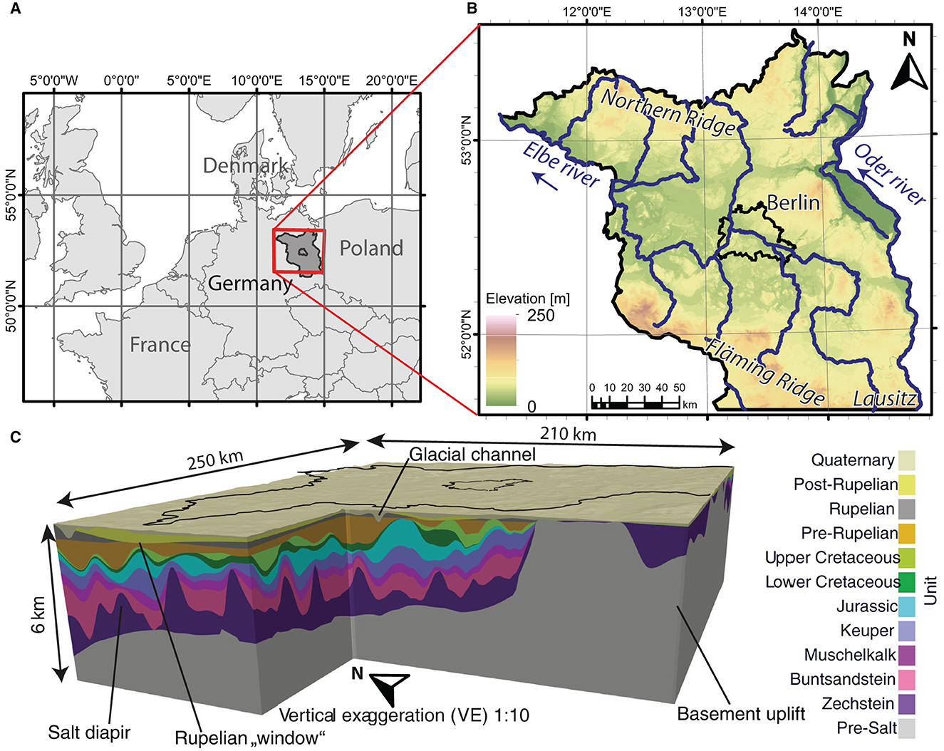
Figure 1. (A) Location of the study area; (B) topographic map; (C) 3D view of the structural model. Black outline follows Brandenburg administrative boundary, except the southern latitudinal edge, which corresponds to the model 3D model limit.
The lowermost model unit includes all formations below the Zechstein salt: the Paleozoic basin fill (Rotliegend sandstone of Permian age, Permo-Carboniferous volcanics, and Carboniferous molasses) is lumped with the Variscan basement, given the high consolidation state and low permeability of these units (see Section 2.4). These rocks are overlain by the Upper Permian Zechstein formation, which dominantly consists of halite with some anhydrite and carbonate. Salt tectonics resulted in numerous salt diapirs, pillows, and walls from post-depositional mobilization, with vertical thickness locally reaching up to 4,000 m. Rim synclines around these salt structures provided accommodation space, which have been filled by Mesozoic-Cenozoic sediments (Scheck-Wenderoth and Maystrenko, 2013).
Stratigraphically above the Zechstein, the lower Triassic Buntsandstein unit is the deepest regional aquifer considered in the model. This succession, dominated by non-marine sandstones and siltstones, is an important target for deep geothermal energy in the NGB (Huenges and Ledru, 2011; Franz et al., 2018). Above it, the middle Triassic Muschelkalk unit, composed of limestones and interbedded marls, acts as a regional aquitard. The overlying units, Upper Triassic Keuper, Jurassic, Lower Cretaceous, Upper Cretaceous, and pre-Rupelian Tertiary, have a heterogeneous composition with permeable sediments represented by sand, silt, and limestone. These deposits form a single brackish to saline aquifer megacomplex, with salinity increasing with depth from ~1 g/l to >200 g/l (Gaupp et al., 2008). These saline aquifers are a potential target for a number of subsurface utilization projects (geothermal energy, aquifer thermal energy storage, H2 storage, CO2 sequestration; Bruhn et al., 2023). Due to salt movements, basin inversion, glacial erosion, and postglacial isostatic rebound, the thicknesses of each individual unit vary significantly with local manifestation of non-deposition and complete erosion of stratigraphic units.
The Keuper-to-pre-Rupelian Tertiary complex is overlain by the Rupelian Clay unit, which acts as the main aquitard separating the freshwater aquifers above from the saline aquifers below. The Rupelian aquitard is eroded locally, providing domains for cross-formational flow between the Tertiary—Quaternary section above the Rupelian Clay and the units below the base Rupelian unconformity. These hydrogeological windows are the widest in the southern part of the study area, where a greater stratigraphic succession is missing, such that Quaternary deposits lay directly on Paleozoic rocks (Figure 2A).
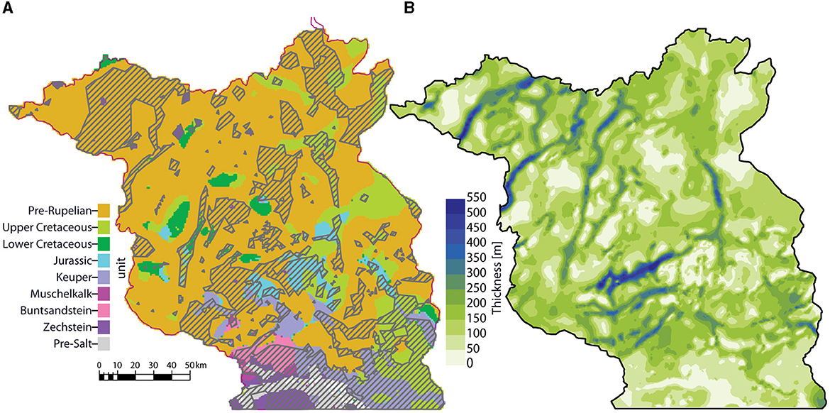
Figure 2. Geologic controls on groundwater flow, as extracted from the 3D geological model, relevant surface-groundwater interactions: (A) Rupelian subcrop map with dashed areas corresponding to absence of Rupelian aquitard; (B) Quaternary thickness map, where thicknesses of 300–550 m correspond to SW-NE-oriented glacial channels.
The post-Rupelian Tertiary unit is mainly composed by fluvial and lacustrine clastic deposits. Tertiary lignite has been mined in the region since the end of the eighteenth century, with large open-case mines altering groundwater quality and levels from the second half of the twentieth century (Benthaus and Totsche, 2015; Tissen et al., 2019). Quaternary is the uppermost modeled unit, with its top defined by the surface topography. Lithologically, it consists of glacial, fluvio-glacial, and alluvial sands, silts, and muds with a total thickness of up to 540 m (Figure 2B). Maximum thickness is reached within NE-SW oriented glacial channels, likely formed by subglacial meltwater erosion (Sirocko et al., 2008). Quaternary channels incised deep into underlying Tertiary rocks, sometimes eroding the Rupelian Clay.
The present-day relief in Brandenburg has been shaped by the last three Pleistocene glacial and intraglacial cycles (Stackebrandt and Manhenke, 2010). Consequently, elevated belts of moraines align preferentially along WNW-ESE oriented axes, separated by wide ice-marginal valleys. Absolute elevations range from 0 to 200 m a.s.l., with elevations above 50 m being typical for plateau belts, and those below characteristic for valleys and floodplains. Large differences in height occur over short distances (Stackebrandt and Manhenke, 2010).
We have assigned constant physical properties to each stratigraphic unit, chosen consistently with its predominant lithology (Table 1). Despite recent advances in facies-dependent petrophysical characterizations for specific sites and formations within the NGB (BGR-SGD, 2019; Norden et al., 2023), we chose to rely on a homogeneous parameterization due to the regional span of the model, which together with an uneven data coverage hinders a more differentiated litho- or sequence-stratigraphical mapping at a basin scale. The selected rock properties are consistent with published parametrized models of the same geographic area and with the results of sensitivity analyzes conducted herein (Noack et al., 2013; Frick et al., 2019). Permeability is typically much higher parallel to bedding than orthogonal to it. We approximated this anisotropy, by orienting principal directions of permeability vertically and horizontally. Assigned vertical component (Kz) is set one order of magnitude smaller than lateral components (Kxy). This is a common assumption for stratified sedimentary materials, while Kz/Kx(y) ratios measured in cores may vary substantially depending on mineralogy and lithology (Domenico and Schwartz, 1997). We assign an isotropic permeability of 1e-19 m2 to both, the pre-Salt and Zechstein units, which act as a natural impermeable base to fluid flow, while still allowing for heat conduction. Consequently, the model does not account for groundwater movement in Rotliegend sandstones, marginal carbonate-dominated facies of Zechstein formation, or weathered basement uplifts. Due to its composition, the Zechstein unit has a higher thermal conductivity than the rest of the basin fill, with salt structures acting as chimneys for conductive heat transfer on a basin scale (Noack et al., 2013).
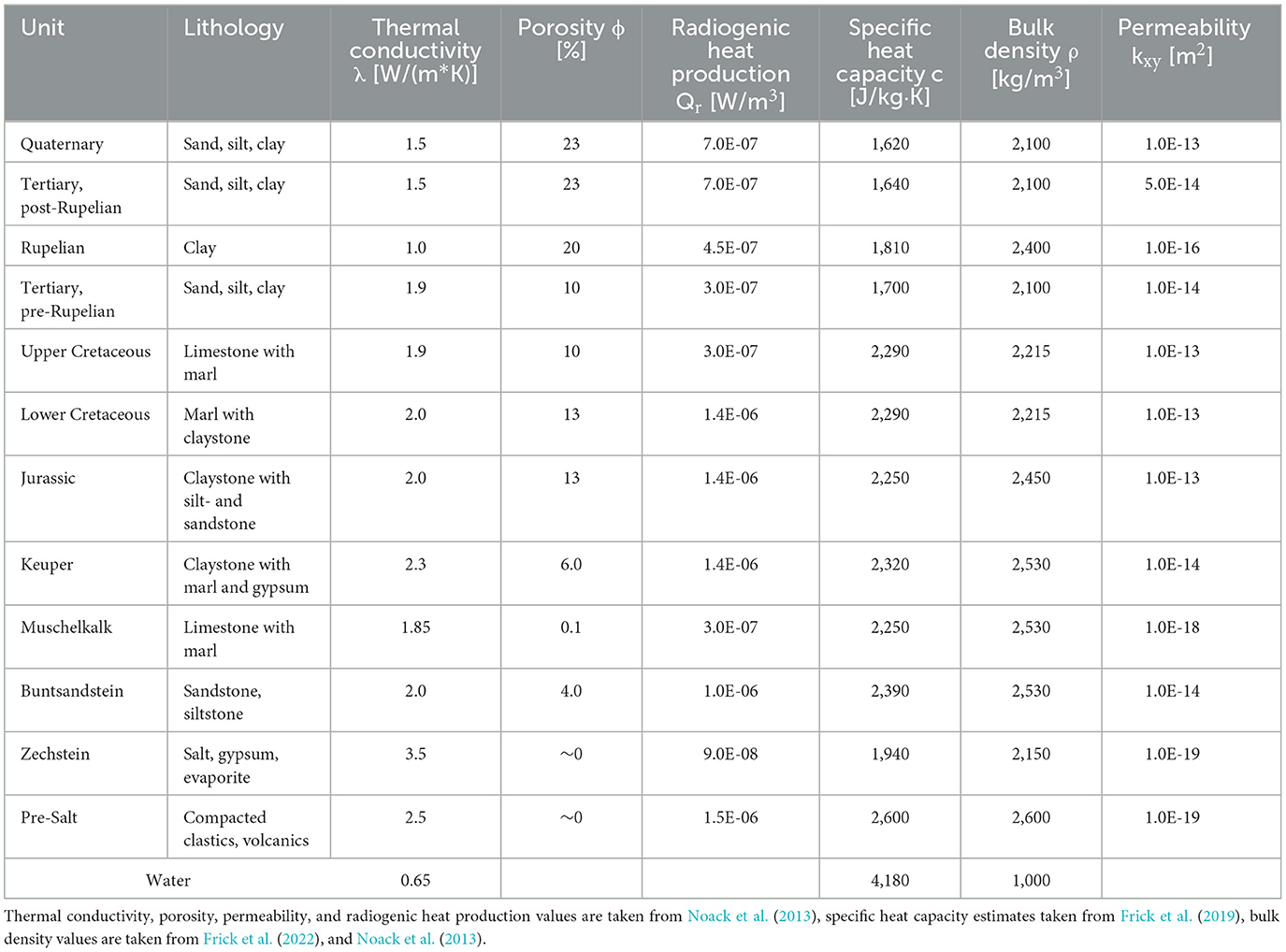
Table 1. Petrophysical properties of the model units assigned in the numerical simulations.
Fluid properties are considered constant for all units (Table 1), with viscosity 0.001 Pa·s and fluid modulus 2.18e+9 Pa, except for the Quaternary unit, for which we set a higher fluid modulus equal to 2.18e+5 Pa to approximate the higher storativity in the aquifer with unconfined conditions, consistent with an equivalent specific yield of 0.1. In our study, we neglect variations in fluid density and viscosity with depth due to salinity and temperature stratification. Our choice stems from previous studies, which demonstrated how density driven free convection is unlikely to be a significant heat transport mechanism in the NGB (Kaiser et al., 2011). Given the modeled temperature range of interest (~200°C), an ~1 order of magnitude variations in water viscosity is expected (Kestin et al., 1978). Therefore, we may underestimate the hydraulic conductivity at greater depths. However, the impact of such variations in fluid viscosity on the regional Darcy flux can be considered of secondary relevance than that resulting from the heterogeneous permeability field, which also decreases with depth.
We have conducted all simulations presented below with GOLEM, a Finite Element Method (FEM) modeling platform for thermal-hydraulic-mechanical and non-reactive chemical processes in fully-saturated porous media (Cacace and Jacquey, 2017). GOLEM relies on a pressure-based formulation to describe the groundwater mass balance as:
where ϕ–porosity, Kf–fluid modulus, ρf —fluid density, k—permeability, μf–fluid viscosity, g—gravitational acceleration. The first term of Equation 1 describes the change in water storage under the assumption of incompressible rock matrix), and the second term describes the gradient of Darcy flux.
Equation 1 is implicitly coupled with an equation describing the conservation of the internal energy of the porous system, considering change in heat storage, as well as advective and conductive transport components as:
where c—specific heat capacity, b and f subscripts denote bulk or fluid properties, T—temperature, λ–thermal conductivity, Qr—rate of radiogenic heat production.
An earlier coupled simulation study in NGB suggested that free convection (density-driven flow due to temperature and/or salinity gradients) can be considered as a secondary source of groundwater flow acting only locally within the most permeable and thick Mesozoic section and in the absence of any significant hydraulic gradients (Kaiser et al., 2013). Since our study focuses on climatic drivers over a time window of six decades, which will affect primarily the shallow freshwater aquifers, we decided to neglect double-diffusive convection in our simulation set-up.
When converting the input geological model into a 3D FEM mesh, each modeled stratigraphic unit has been vertically subdivided into four computational layers, while a higher resolution has been applied to the Quaternary unit, which was refined by a factor of 10 to better approximate the dynamics near the surface-subsurface interface. The lateral resolution of the FEM mesh has been kept to 1 km x 1 km as in the original geological model. The final model, divided into 54 computational layers, consists of 1.59 million nodes, giving a total of 3.18 million degrees of freedom.
Equations 1, 2 form an initial boundary value problem, the closed form solution of which requires to specify a set of initial and boundary conditions. We have first derived steady-state conditions by solving separately for the hydraulic (Equation 1) and the thermal (Equation 2 with only the conductive term included). These uncoupled steady-state simulations have been used as initial conditions to run a coupled pseudo-transient simulation, the results of which have been later imposed to initialize the pore pressure and the temperature in the final transient simulation.
For the steady state runs, we assume hydrostatic conditions with respect to a spatially variable hydraulic loading at the surface as given by a fixed hydraulic head. The initial distribution of hydraulic heads for the Quaternary unit across the study area is based on ~100 groundwater level measurements taken in 1953 together with a trend from the water table contour map of 1999 (Landesamt für Umwelt Brandenburg, 2020). The resulting hydraulic heads grid has been converted into a pressure boundary condition (Figure 3A) as:
where P is the assigned pressure at the top boundary, P0 is 1 bar (pressure at the water table), Z is ground elevation, h is the hydraulic head.
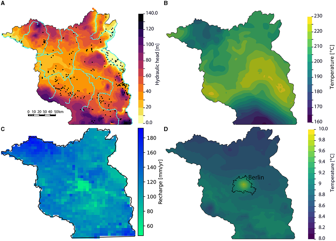
Figure 3. Source grids used for boundary conditions assignment: (A) pressure at the top boundary with groundwater level measurement points (Landesamt für Umwelt Brandenburg, 2023) and river boundary conditions; (B) basal temperature at −6,000 m a.s.l.; (C) mean annual groundwater recharge 1953–2014; (D) mean surface temperature 1953–2014 (Deutscher Wetterdienst—Climate Data Center, 2021).
To better approximate the shallow groundwater dynamics, we additionally integrate the 15 longest rivers in Brandenburg as a node set to which we assign a Type I (Dirichlet) pressure boundary condition with a constant value of 1 bar, thereby forcing groundwater level to match the model top at these locations.
We close the side edges of the 3D model, therefore assuming that no significant lateral flow or heat transport occurs into or out of the domain. This assumption particularly applies for the shallowest aquifer, for which the Oder river in the east, the Elbe river in the west, and watershed divides in the north and south act as natural hydraulic no-flow boundaries (Figure 1B). There is a higher potential of outflow from the deeper aquifers, that, according to regional geology, dip northward, extending beyond the model domain, while onlapping onto the basement high to the south. The impact of our choice of side boundary conditions is discussed further in Section 4.4. A Type I temperature boundary condition is assigned along the top surface as derived from grids of monthly averaged daily air temperature 2 m above the ground from the German Weather Service (Deutscher Wetterdienst—Climate Data Center, 2021) and averaged over a period of 1951–1953.
Along the base of the model, we assign no flow and a Type I temperature boundary conditions (Figure 3B). Given the extremely low permeability at a depth of −6,000 m, flow through this boundary can be indeed considered as negligible. The basal temperatures have been extracted from a lithosphere-scale thermal conductive model of Brandenburg, which has been additionally validated against temperature measurements from deep exploration wells (Noack et al., 2012). Basal temperature ranges from 230 to 160°C, reflecting difference in the thickness of the crystalline crust and the sedimentary cover. Lower temperatures in the southwest corner are caused by an almost complete absence of any sedimentary cover on top of the uplifted basement (Figure 1C). Without insulation from the low-conductive sediments, highly conductive basement rocks efficiently dissipate heat toward the surface. Higher temperatures in the center correlate with a thicker felsic upper crystalline crust, generating more heat from radiogenic decay, covered by 3–5 km of insulating clastic sediments (Scheck-Wenderoth and Maystrenko, 2013).
In a second step, we use the results from the uncoupled thermal and hydraulic runs as initial conditions to a pseudo transient coupled thermo-hydraulic simulation, that is, a transient simulation which has been run till reaching equilibrium conditions. For this run we impose the same set of boundary conditions as described above. We set a constant timestep of 1,000 years and considered steady state conditions if the maximum change in temperature and pressure per simulation step drops to values lower than 0.1°C or 10 kPa, respectively. Steady-state conditions were achieved after ~120,000 years.
In the final simulation step, we take the output of the pseudo transient coupled simulation as initial conditions for the transient thermo-hydraulic simulation to quantify the influence of time-varying climate-driven surface forcing conditions over the period from 1953 to 2014, with a timestep of 1 month. This period was chosen due to availability of all input data required to compute recharge in a hydrological model. As a caveat, the onset of the transient simulation coincides with increasing groundwater abstraction due to population growth and mining activities in Brandenburg.
The temperature boundary conditions imposed along the top surface have been derived from a spatial interpolation of the monitored monthly air temperature time series (Deutscher Wetterdienst—Climate Data Center, 2021). Mean surface temperatures across the study area vary between +8.5 and +10°C, with a decreasing trend from south to north and a positive thermal anomaly in the center of the study area associated with the urban heat island of the capital city of Berlin (Figure 3D). Time series of the surface temperatures indicates an annual difference between the coldest and the warmest months varying from 15 to 21°C, and an increase of mean annual temperature of ~1°C during the simulated period (Figures 4A, B).
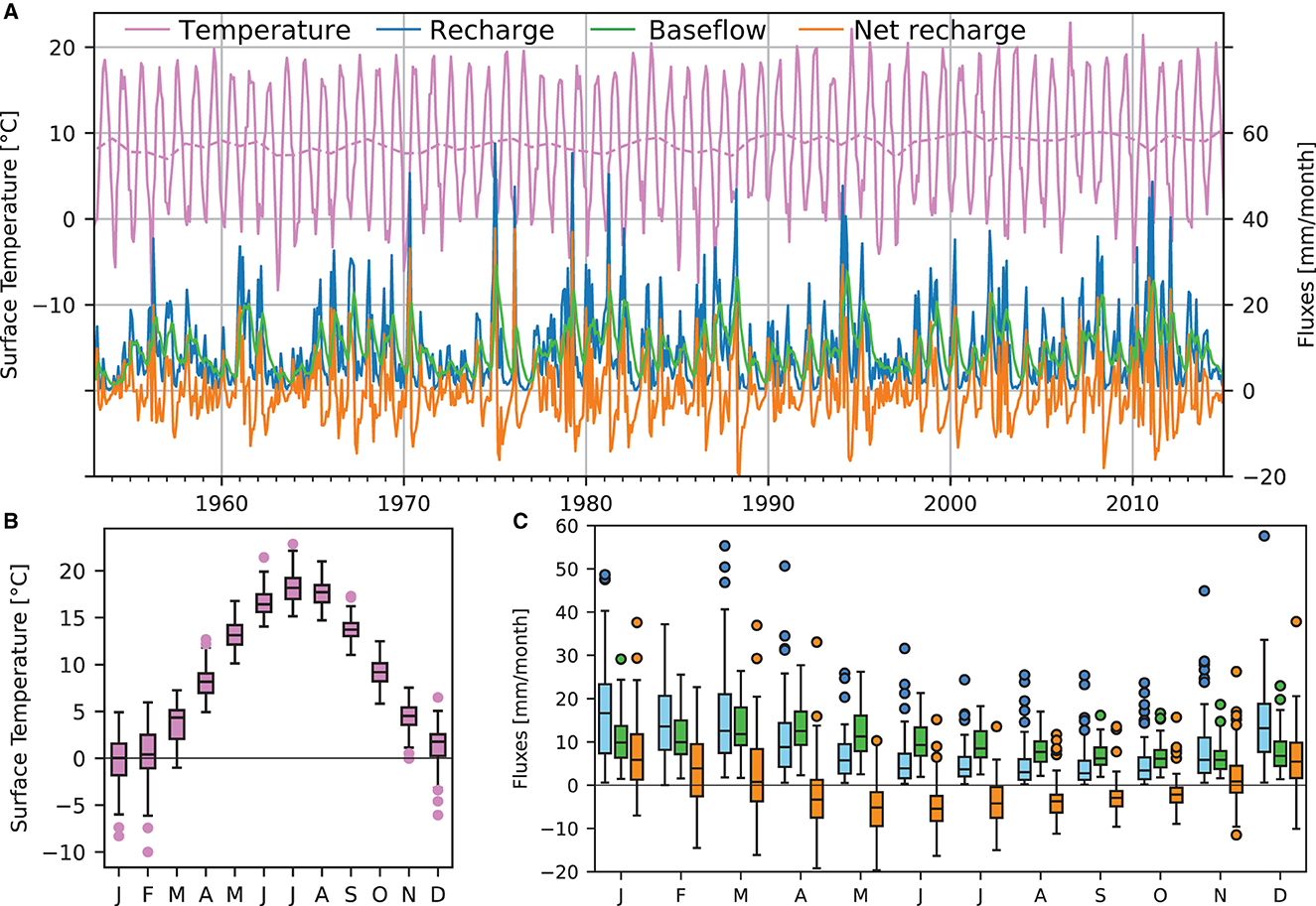
Figure 4. Hydrometeorological monthly time series, mean values across the study area. (A) Surface temperature and mHM output fluxes; dashed line corresponds to annual temperature mean; (B) boxplots of monthly temperature (B) and mHM output fluxes (C) across the study area for the entire simulation period.
Many hydrologic models that employ water balance components, climatic data, and physics of the unsaturated zone, are able to simulate groundwater recharge from watershed to global scales. For the current study, we make use of the mesoscale Hydrological Model (mHM; Samaniego et al., 2010). mHM is a spatially distributed hydrologic model that uses gridded observed surface temperature and precipitation as inputs. We make use of the results from a Germany-wide realization of mHM to derive time and space varying water fluxes, which we translate into boundary conditions at the top of our groundwater model. The output of the mHM model consists of monthly 5 km x 5 km grids as used in Rakovec et al. (2016) and Samaniego et al. (2019) covering the period 1953–2014, with the following response fluxes relevant to the current study, as defined in Samaniego et al. (2010):
where C is percolation from the soil layers to the groundwater reservoir (i.e., groundwater recharge), [mm/d]; q4 is baseflow, [mm/d]; β22 is an effective percolation rate [1/T], which depends on the hydraulic conductivity of the soil; β23 is a baseflow recession rate [1/T], which defines how the release of water from the groundwater reservoir to surface runoff in the stream network must be distributed over time; x5 defines the amount of water storage in the lower soil reservoir, expressed in equivalent water height, [mm]; and x6 the amount of the water storage in the groundwater reservoir, [mm]; t is time index for each time interval.
mHM is a process-based bucket-type hydrological model with a spatial regularization on regular grids. All hydrological processes are calculated first separately for each individual grid. The flow from different runoff components (e.g., fast and slow interflow and baseflow) is then routed from cell to cell, according to the largest topographic gradient as derived from the digital elevation model. The spatial parameterization approach (multiscale parameter regionalization, MPR) leads to spatially consistent outputs of hydrological states and fluxes (Samaniego et al., 2010; Kumar et al., 2013). There is no subsurface lateral flow redistribution between grid cells in mHM, though this may be relevant especially at the regional scale, where groundwater recharge and discharge areas are usually situated away from each other (Jing et al., 2018).
We apply the net recharge flux, being the difference between recharge and baseflow fluxes in an mHM cell at any given time, as a Type II (Neumann) pressure boundary condition, where positive net flux indicates that recharge outweighs baseflow, and vice versa (Figure 4A). Given that for each grid cell of mHM the sole source of baseflow is recharge in the corresponding cell, over a sufficiently long period the net flux will be close to zero. It follows that cells with a high recharge flux also have a high baseflow component and vice versa. Lateral groundwater flow along a topographic gradient is not represented in the hydrological model (no lateral/horizontal fluxes between adjacent model cells). To alleviate for this limitation of the hydrologic model and to allow for lateral groundwater flow we have integrated the major rivers in the study area into the groundwater model with a constant pressure (1 bar), ensuring the presence of a regional hydraulic gradient at all times.
For the modeling and data analysis, we limited the mHM output to the spatial extent of the 3D geological model, and interpolated the data onto the mesh. Long-term recharge increases in the NW direction up to a maximum of >160 mm/a and spatially correlates with a seaward increase in precipitation (Figure 3C). Southern Brandenburg, characterized by a hilly terrain, also has relatively higher recharge rates. The lowest recharge (<60 mm/a) is modeled for the Berlin metropolitan area due to its urban land cover.
Figure 4C illustrates the 12-month long time series derived from averaging the mHM fluxes across the whole study area and the entire simulation period. Groundwater recharge peaks between January-March, and reaches its minimum in August-September, being therefore temporally linked to the seasonality of evapotranspiration rather than precipitation. The peak in baseflow typically lags 1–3 months behind the peak in recharge followed by a 7–11-month long recession. According to the sign of net recharge flux, groundwater typically gains storage from November to March and loses storage from April to October.
The final output of thermo-hydraulic simulation contains modeled pressure and temperature at every mesh node for monthly timesteps. We use the open-source ParaView software (Ayachit, 2015) for post-processing and analysis, including back-calculation of hydraulic heads from the pressure field.
We validated the model results against published groundwater level and temperature data. The groundwater monitoring network of Brandenburg comprises ~1,900 observation wells and piezometers with daily to quarterly measurements (Landesamt für Umwelt Brandenburg, 2023). While the earliest groundwater level records date back to the 1920's, a more uniform spatial coverage (>500 localities) is only available from 1970 onward, making possible to have a higher-confidence validation dataset for the modeled time series (Figure 3A). Observation wells tap exclusively Quaternary and Tertiary unconfined, confined, and perched aquifers. Differences in well construction, spatial clustering of sometimes conflicting data, and uncertainty in the well penetration levels make it challenging to reconstruct consistent potentiometric maps over the entire Berlin-Brandenburg region for every timestep. We therefore utilize a limited set of gridded equipotential line maps that incorporate quality-controlled groundwater and surface water data (Landesamt für Umwelt Brandenburg, 2020), while relying on individual wells for time series analysis.
Groundwater temperature is monitored in ~200 observation wells in Berlin and ~200 wells in Brandenburg and is limited to 80 m below ground (SenStadt, 2020). Static measurements in the deeper pre-Cenozoic section come from corrected bottom-hole temperatures and repeated temperature logs in ~50 petroleum exploration wells (Förster, 2001; Norden et al., 2008). They have been previously used for calibration of steady-state models of Brandenburg (Noack et al., 2013), from which we derived the lower thermal boundary condition for calculating the deep thermal field in the present study (Supplementary Figure 1).
The aim of this model realization is to capture equilibrium groundwater conditions under a fixed, though spatially variable reference head and surface temperature prior to the onset of the transient simulation (1953). As such, it provides a first-order description of the groundwater dynamics and resulting thermal field through the entire stratigraphic section without considering the influence of climatic cyclicity (i.e., neglecting seasonal changes in recharge and surface temperature) or continuous climate warming.
Analytical models of gravity-driven flow in a homogeneous isotropic basin suggest that the superposition of the regional slope and local water table relief is responsible for forming flow cells that differ in distance between recharge and discharge areas and their depth of penetration (Toth, 1963). Consequently, groundwater flow in sedimentary basins is often subdivided into regional, intermediate, and local flow systems. In what follows we examine the results based on computed groundwater flowlines and Darcy flux, focusing on three stratigraphic intervals of interest: Buntsandstein, Keuper—pre-Rupelian, and post-Rupelian—Quaternary (Figure 5).
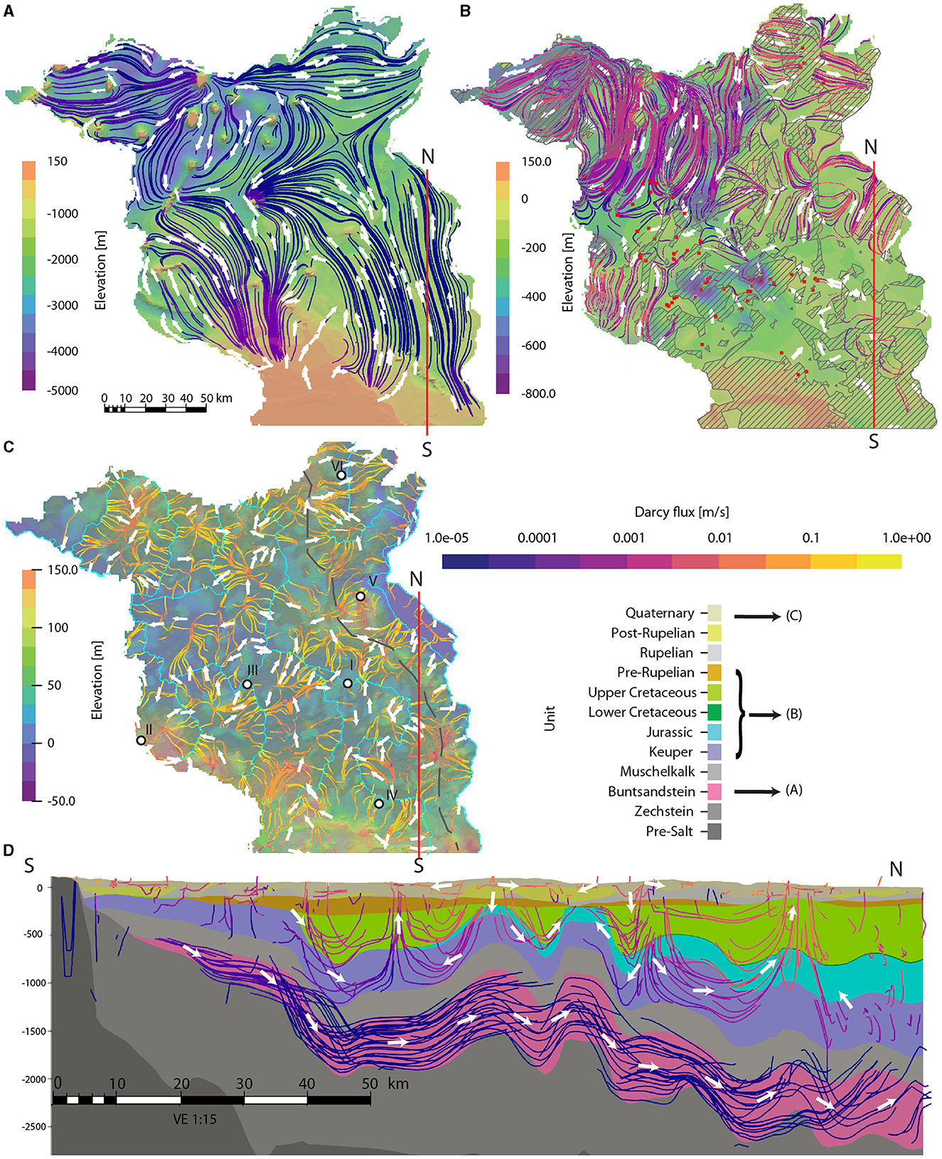
Figure 5. Groundwater flowlines under steady-state conditions: in Buntsandstein (A), in Keuper to pre-Rupelian Tertiary untis (B), in Quaternary (C), in all units along a S-N slice (D). Coloring of the maps show top aquifer elevations. Roman number annotations refer to locations shown on Figures 7, 10. Dashed areas refer to Rupelian windows, arrow glyphs indicate flow direction, streamline color indicate Darcy flux, dashed gray line—Oder-Elbe watershed divide, red squares—evidence of saltwater discharge at the surface as given by Rößling et al. (2010).
As an example of a regional groundwater system, we look at the Buntsandstein unit (Figure 5A), the deepest modeled aquifer, bounded below and above by impermeable Zechstein and Muschelkalk units. The spatial extent of individual flowlines (computed as the distance between the entry and exit points of the groundwater flow) spans over 100 km, indicating a regional, long-distance flow with long residence times. The dominant direction of the flow is from the south to the center and then to the northwest and northeast. Such an orientation is defined by the reservoir dip, which is, in turn, controlled by the basin configuration. In the southern marginal part of the basin, the Buntsandstein is uplifted to < -1,000 m a.s.l., while in the northwestern part it is buried below −3,500 m a.s.l. The Buntsandstein aquifer is likely recharged in the south of Brandenburg, where it lies at depths of < 200 m below ground directly underneath a thin Cenozoic cover in the absence of Muschelkalk and Rupelian aquitards. Following the steeply dipping Buntsandstein, Darcy flux ranges between 1e-4 and 1e-3 m/s, and water can freely flow downward. As groundwater flow becomes dominated by a more lateral component, Darcy flux decreases to 1e-5 – 1e-4 m/s. Groundwater flow is diverted locally, in the northeastern quadrant of the model, where large Zechstein salt diapirs and salt walls are present. Salt structures act as a local gradient anomaly being associated to elevated Darcy flux. Groundwater tends to sink into the salt rim synclines and to rise over salt structures, following the folded topology of the Buntsandstein reservoir. Due to the no-flow boundary along the model edge, groundwater leaves the aquifer via cross-flow to the adjacent units, eventually discharging at the surface. A larger basin model of the whole Northern Europe suggested that this deep groundwater flow actually continues north-west toward the most buried offshore parts of the NGB (Frick et al., 2022).
The intermediate flow system includes units from Keuper to pre-Rupelian Tertiary and lies between two regional aquitards, the Muschelkalk below and the Rupelian above. The thickness of this aquifer complex increases from < 1,000 m south of Berlin to more than 2,000 m in the north-western part of Brandenburg, where fluid circulation is also more active (Figure 5B). Erosional windows in the Rupelian aquitard provide pathways for groundwater cross-flow to and from the post-Rupelian—Quaternary aquifer complex. The intermediate flow system is recharged, where hydrological windows lie below topographic highs, while discharge occurs where the windows are found below topographic lows. Therefore, the flow travel distances structurally depend on the distance between adjacent erosional windows. The presence of saltwater springs and halophilic plants on the surface as mapped by Rößling et al. (2010) is consistent with the upward flow through Rupelian windows in the central and northeastern parts of the study area. Darcy flux ranges from 1e-5 to 1e-2 m/s with highest flux in the permeable Jurassic and Cretaceous units. Individual salt structures cause local diversion of the flow from the shortest path between inflow and outflow points. In rim synclines the vertical flow dominates over the lateral component of the flow.
Groundwater dynamics of the local flow system, that includes post-Rupelian Tertiary and Quaternary units, is fundamentally different from what has been described above (Figure 5C). Higher Darcy flux (1e-2 – 1e-1 m/s) and shorter travel distances lead to shorter groundwater residence times. There is no predominant flow direction or continuous streamlines at the scale of the whole Brandenburg. Instead, the present-day watersheds configuration controls the orientation of groundwater flow, which follows the topographic gradient, from elevated areas (glacial plateaus, acting as watershed divides) toward the nearest adjacent valley or stream. Due to the “hummocky” post-glacial relief of Brandenburg, groundwater forms numerous domains of recharge and discharge. A N-S drainage divide (gray line on Figure 5C) separates groundwater catchments contributing to the Elbe and Oder river basins.
Groundwater levels vary from −5 to 140 m a.s.l. across the study area (Figure 6A). Depth to the water table, calculated as the difference between surface elevation and groundwater level, lies predominantly between 0 and 30 m, with 5% of model cells having a deeper water table (Figure 6B). In places where recharge derived from mHM is abundant, the water table is shallower and the groundwater level shows a preferential correlation with the topographic elevation, i.e., the potentiometric surface replicates the topographic relief. As recharge decreases, groundwater level correlates less with the topography. At surface elevations >100 m, the groundwater level becomes more variable and does not follow the surface relief even in those model cells characterized by a high estimated recharge (Figure 6A). Model cells with a surface elevation to groundwater level ratio >2 can be explained by the additional artificial lowering of the water table from pumping and drainage.
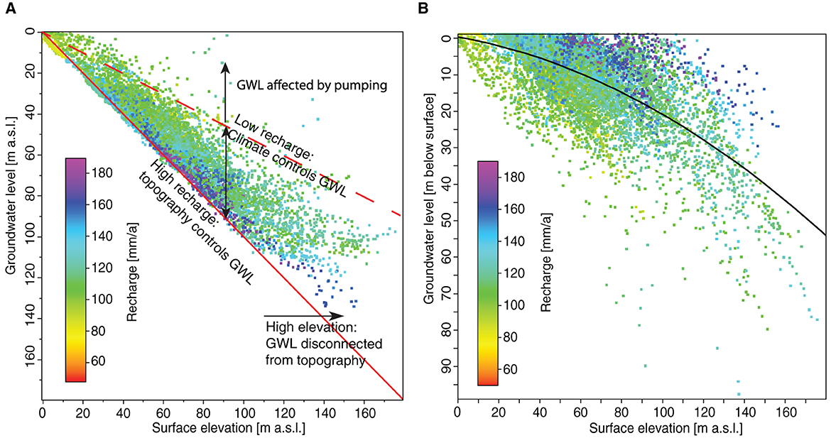
Figure 6. Controls on steady-state groundwater level. (A) Topography and groundwater level elevation, with 1:1 and 2:1 ratios shown as solid and dashed red lines for reference in solid red; (B) topography and depth to water table; a line of best fit shown in black. Each point represents a single grid cell of the groundwater model.
In order to visualize how variations of the imposed boundary condition over time affect the local groundwater system, we plot in Figure 7 time series of computed Darcy flux for two selected locations, on a glacial plateau (point V in Figure 5C) and in a river valley (point VI in Figure 5C). We found that variations in the vertical component of the Darcy flux show a high degree of correlation with variations in the net recharge. In late winter and spring, when recharge is higher than baseflow (i.e., net inflow), the vertical downward component of the Darcy flux is enhanced, while showing an opposite trend in summer and early fall. The lag time between net recharge and Darcy flux peaks at a depth of 25 m below ground varies from 1 to 6 months, being shorter in the valley location. Such correlation is even more evident if looking at specific years characterized by exceptionally high recharge (as in 1994 and in 2002), where we observed a reversal in the vertical flow component in the valley location, otherwise dominated by an upward flow (marked by green boxes in Figure 7). Seasonal changes in groundwater flux magnitudes and directions are limited to the post-Rupelian section: the annual cycle in the surface flux signal does not propagate through erosional windows, as can be seen from steady velocities at −200 m, corresponding approximately to the top of pre-Rupelian unit for both locations. We therefore observe no modification in the regional and intermediate groundwater flow during the whole 62-year time period investigated.
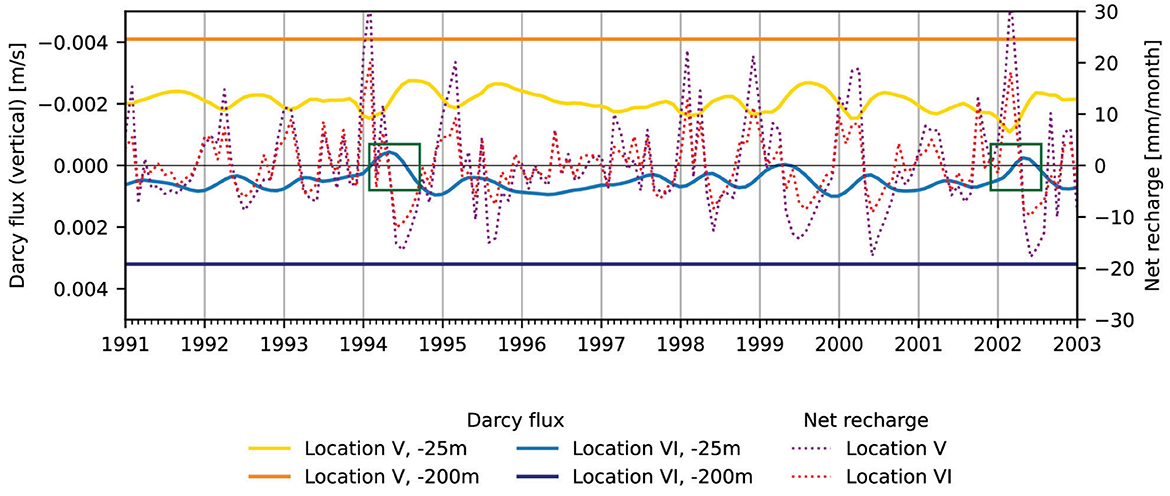
Figure 7. Time series of net recharge flux and simulated vertical Darcy flux at two locations, shown on Figure 5C. Location V is on top of a glacial plateau, while location VI is in a river valley. Positive net recharge flux corresponds to the gain of groundwater storage, negative Darcy flux corresponds to downward flow.
Figure 8 depicts computed differences between modeled and observed water levels at the end of the transient simulation. The Pearson correlation coefficient of 0.98, with a RMSE of 1.92, indicates that the model predicts the observed groundwater level well with +/- 2 m of misfit over the study area. An anomalously high misfit of ±10 m in two localities in the southeast of the study area is associated with lignite mining activity (Lausitz region), which was on the rise until 1985, followed by a gradual closure and recultivation of open-cast mines. To access the coals seams in Tertiary and Quaternary units, the water level had to be lowered by 30–50 m. The area of misfit spatially correlates with depression cones, which extend well over the borders of the opencast mines (Benthaus and Totsche, 2015).
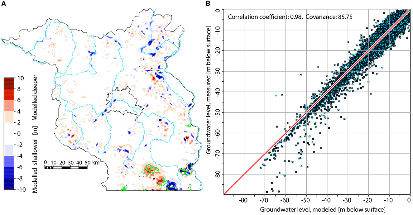
Figure 8. Difference between measured hydraulic heads and those predicted by the transient simulation at the end of the transient simulation. (A) Map (B) cross-plot with each point corresponding to a grid cell of the groundwater model, red line is 1:1 line. Green polygons outline open-cast mines.
In valleys and floodplains, where groundwater level is near the surface and therefore less variable, the misfit between simulated and observed level lies within a confidence interval of ± 2 m. A misfit up to +8 m is found around topographic heights, where the groundwater level is also deeper. According to hydrogeological mapping, near-surface porosity and permeability is lower on the highs than in the river valleys (BGR-SGD, 2019). Therefore, we can anticipate higher magnitude fluctuations in these regions.
The amplitude of hydraulic head variations in the model is a function of the net recharge flux at the upper boundary and of the aquifer storativity. As commonly done, we can also make use of the relationship that estimates recharge following a Water Table Fluctuation (WTF) method (Healy and Cook, 2002). For a specific yield of 0.1, as the one assumed for the Quaternary unit, and given recharge rates as typical for Brandenburg (60–180 mm/yr) the expected seasonal range of water table fluctuation, i.e., the difference between the highest and the lowest position of the water table in a given year, is between 0.3 and 0.9 m, assuming an equal duration of rise and fall of 6 months. If we compute the seasonal fluctuations based on all measured wells, we arrive at values of 0.17 m [10th percentile (P10)], 0.68 m (P90), and 0.41 (P50). Modeled average seasonal fluctuations in the groundwater level range between 0.25 m (P10) and 0.48 m (P90) with P50 of 0.36 m, thereby in agreement with measured values. We note a positive correlation between magnitudes of seasonal fluctuations and recharge, with the maximum fluctuations in NW and SE, and the lowest fluctuations in the center (Berlin) and in E-NE (Figure 9). We also note an overprint of the local geology: in the Quaternary glacial channels the average seasonal fluctuations are lower than outside of the channels because of the greater porosity and higher storage.
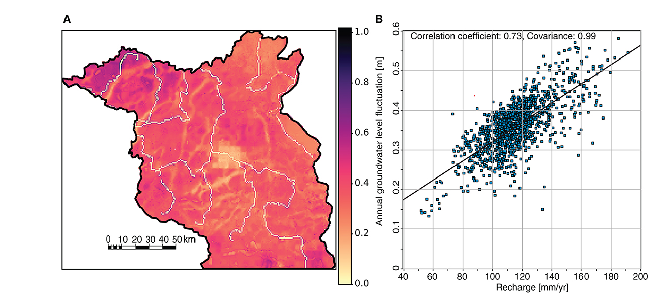
Figure 9. Average groundwater level difference between an annual maximum and minimum for the transient simulation: (A) spatial distribution of the seasonal groundwater level fluctuations. (B) Cross-plot between annual groundwater level fluctuation and recharge, with each point corresponding to a grid cell of the groundwater model; black line is a line of best fit.
To further validate the model outcomes, we cross-plot the simulated groundwater level time series against measurements for several representative observation wells, within different geomorphological and hydro-geological settings (Figure 10).
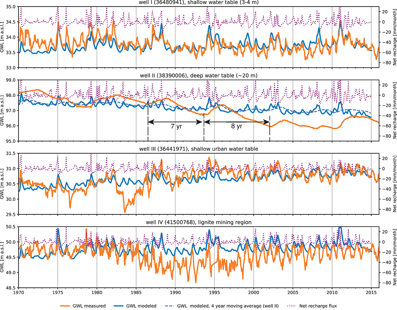
Figure 10. Groundwater levels (GWL): measured and modeled, and net recharge flux time series for selected observation wells shown on Figure 5C. All presented wells are screened in the Quaternary unit. Numbers in the brackets refers to well ID in Brandenburg Water Information Platform (Landesamt für Umwelt Brandenburg, 2023), from where the monitoring data is available for download.
Well I is representative of a river valley or floodplain setting, characterized by a very shallow water table (0–5 m below ground). The wellhead location is ~0.5 km away and 4 m above a river. We observe a good agreement between modeled and measured groundwater level behavior with short-wavelength fluctuations correlating to the assigned net recharge flux. The seasonal magnitude in groundwater level change ranges between 0.1 and 1 m with highest levels in spring and lowest in late summer—early fall. Our model also captures years with exceptionally high levels (e.g., 1975, 2011) and the extended periods of low level running throughout 1989–1994. Local disagreements between model and observations of up to 0.5 m can be seen in the period between 1972 and 1974. We also note that the modeling results can capture the longest observed period of sustained decline in the levels from 2011 to 2015.
Well II is representative of a hilly terrain setting, characterized with a deeper water table (>20 m below surface). The well is located on the Fläming ridge, SW Brandenburg. We note a poor correlation between observed and modeled groundwater level dynamics, with the measurements lacking any clear indication of seasonal variability but rather following a 7–8-year cycles with a smooth and likely delayed response to large recharge pulses (arrows on Figure 10). This smoothed response is likely due to the travel time of infiltrating meteoric water through a thicker unsaturated zone, a process not explicitly considered by mHM, and therefore not reflected in the net recharge or modeled level time series. Indeed, after applying a moving average filter with a 48-month window to the modeled heads, we have been able to reproduce the periodicity in the modeled time series (dashed line). We also note a ~2 m groundwater level decline as monitored over the entire time window, while the modeled level exhibited a weaker long-term trend. A stronger decline of the measured levels could be explained by the fact that groundwater has been used for crop irrigation in the surrounding area on top of the Fläming ridge since the 1990's, representing an additional sink which is not captured by our model (NABU-Brandenburg, 2021).
Well III represents an example of long-term water table behavior in an urban area (SE Potsdam). The water table is shallow, 3–4 m below ground. During two periods, in 1976 and 1983, modeled levels deviate from the historical record by up to +0.7 and +1 m, respectively. The modeled trend is solely driven by climate forcing, as the groundwater model does not include other sinks, such as pumping. Conversely, the climatic variability of the measured levels shows a clear interference typically caused by a drawdown from groundwater abstraction. The affected time period is indeed associated with the maximum population growth and new housing development in post-war Potsdam. The average annual city water consumption rose during these times from 36 k m3/d in 1967 to its peak of 65 k m3/d in 1988 before dropping sharply in the 1990's (Zühlke, 2018). In the remaining period (from 1988 to 2014) modeled and observed groundwater level behavior match, an indication that by that time groundwater extraction has stabilized, and that the annual hydrologic cycle has become the primary control to the observed fluctuations.
Well IV denotes the influence of open-cast mining on groundwater levels in Brandenburg's Lausitz region. The observation well with a shallow water table (1–2 m deep) is located 3 km away from an ex-coal mine, which was in operation between 1983 and 1996 (Seese-Ost), and then was partially filled with water to form artificial lakes (lakes Bischdorf and Kahnsdorf). The measured levels began declining in 1985, followed by a recovery since 1995. In the same period, modeled levels exhibited only seasonal fluctuations. The maximum deviation between measured and modeled levels of 1.1 m was reached in 1992. Despite the strong anthropogenic overprint, recharge influence on groundwater levels was not suppressed as seen from peak levels in 1994 and relatively stable low levels during a dry period in 1996–1997.
The steady-state thermal field beneath Brandenburg has been extensively studied in previous works (Noack et al., 2012, 2013), which compared the effect of basement heterogeneity on the conductive heat transport and modifications to the resulting basin-wide thermal regime by additional advective forces in the sedimentary section. Here we focus on discussing the transient behavior of shallow groundwater temperatures due to the spatially and temporally varying recharge and surface temperatures.
In doing so, we based our analysis on temperature maps extracted at different depths relative to the surface (500, 100, and 25 m), rather than depth maps relative to sea level or top aquifer maps since this enables more consistently quantify the overprint of surface processes on the thermal distribution. We therefore compared the temperature at the start (1953) and the end (2014) of the transient simulation as well as the difference between summer and winter seasons. We further note that at 500 and 100 m below the surface, the temperature distribution does not exhibit any significant temporal fluctuation, so for those intervals we discuss only the initial-state maps (Figure 11).
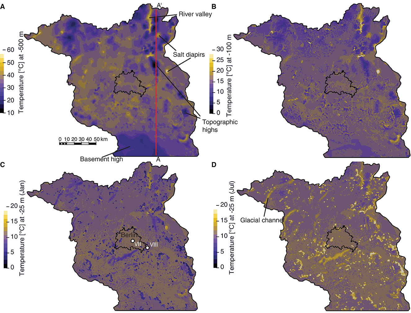
Figure 11. Temperature at 500 m (A) and 100 m (B) below ground at the start of the simulation (no seasonal difference) and average temperature in 1980–2014 in January (C) and in July (D) at 25 m below ground. A-A' refer to the cross-sections on Figure 12; VII, VIII—well locations, for which temperature time series are presented on the Supplementary Figure 2.
At depths of 100 m and greater, temperature patterns are primarily the result of contrast in thermal rock properties between salt, basement and the sedimentary overburden (Figures 11A, B). Lower temperatures in the south are caused by an uplift of the highly conductive crystalline basement in the presence of a thin sedimentary cover. In the rest of the study area, a thick sedimentary cover provides enough thermal insulation to accumulate heat and maintain relatively higher temperature (Figure 12A). The presence of small-wavelength positive thermal anomalies can be associated with occurrences of Zechstein salt structures acting as conductive heat transport chimneys, leading to a dipole shaped heat anomaly: on top of the salt structures, the temperatures are increased due to heat refraction within the highly conductive salt rock and then “trapped” by the less conductive post-Zechstein sandstones, mudstones and limestones.
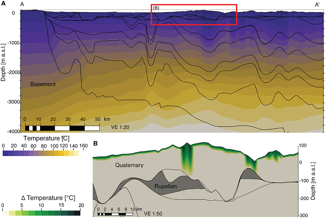
Figure 12. (A) Steady-state temperature distribution in the basin. (B) Average temperature difference between January and July (1980–2014). Location of cross-sections shown on Figure 11.
The additional role played by heat advection from imposed pressure (hydraulic head) gradients can also be noticed at all depth levels. Low-wavelength negative temperature anomalies could be associated to domains characterized by higher hydraulic heads, characteristic for topographically elevated areas (NW, NE, and the south), where hydraulic gradients drive downward flow (recharge areas). Most of these anomalies have a circular shape, and they don't align spatially with hydrogeological windows in the Rupelian aquitard. An opposite thermal signature occurs, for example, below a N-S river valley with lower heads in the NE corner of the model, where upward groundwater flow causes a local warming.
At depths shallower than 100 m, the temperature distribution carries both geological and climatic signatures. For example, at 25 m below ground, the mean temperature for January is +9.9°C, and for July it is +10.8°C (Figures 11C, D), while mean air temperature is −0.2°C and +18.2°C, respectively. The basement high in the SW quadrant and elevated areas with higher head in the east and northwest cause a relative cooling down by 1–1.5°C below the background. Above shallow salt diapirs and in the deeply incised valley in the northeast, temperatures are above the average, reaching up to +15–20°C. Additionally, we note a northward cooling trend of 0.5–1°C, which resembles the pattern of the average surface temperature imposed as the upper boundary condition (Figure 3D).
According to the analytical solution proposed by Stallman (1965), the magnitude of seasonal surface temperature change and total thermal conductivity provide first-order control to the depth to the neutral zone, defined here as a depth where seasonal temperature fluctuations can be considered as negligible (< 0.1°C), while the additional advective component due to downward or upward flow is capable of deepening or raising its depth level. Based on the Quaternary rock properties and the annual average delta in surface temperature for Brandenburg (18°C), the top of the neutral zone is expected to be at 20 m below surface, with the additional effect from downward groundwater flow of 0.01 m/d lowering it to 30 m below surface. Monthly temperature-depth profiles measured in a selection of wells in Berlin find the top of the neutral zone, between 15 and 20 m below ground (SenStadt, 2020). Accordingly, the comparison of July and January temperature distribution at 25 m below ground reveals that most of the study area exhibit no or minimum seasonal change (Figures 11C, D). Patchy areas where the seasonal difference is well-pronounced could be linked to higher heads (Figure 3A) and to glacial channels, where the porous Quaternary unit is the thickest. However, we must note that the effect of surface temperatures within the channels is likely to be overestimated due to the lower vertical mesh resolution. Thirty-five percent of the cells in the uppermost model layer have a thickness >15 m, and 15% of the cells >20 m. Thus, the vertical resolution does not allow to entirely map the top of the neutral zone or temperature at the water table. This said, we can nevertheless determine areas where the seasonal fluctuations propagate substantially deeper than the first computational layer (Figure 12B). Seasonal fluctuations, reaching a maximum depth of 100–150 m, are associated with higher hydraulic gradients (their magnitudes being proportional to the imposed flux), and occur almost entirely within the Quaternary unit, with the Rupelian aquitard effectively limiting the downward propagation of the advective front.
In order to analyze the climate-induced warming effects over the 62-year period, we calculated the difference in the average groundwater temperatures between the last and first 3 years of the simulation and looked at this difference at the depth of 25 m below surface (as a proxy for a top of the neutral zone) (Figure 13A). In most of Brandenburg, the temperature increase is < 0.17°C, i.e., the temperature below the neutral level was not significantly affected during the simulation timeframe. A scattered groundwater heating of up to 2°C at this depth level is observed only locally across Brandenburg and it is associated with elevated hydraulic heads, being additionally facilitated in case of reduced thickness of the Quaternary unit thus forcing flow downward around less permeable underlying rocks (post-Rupelian Tertiary and Rupelian; Figure 13B). Such mechanism can propagate the six decades-long groundwater heating signal of at least 0.2°C to the depths of 150 m below the surface. In instances where these advective forces overlap with hydrogelogical windows, the warming signal may propagate deeper into the saline aquifers, where the second regional aquitard, the Muschelkalk, provides an additional barrier to the advective front.
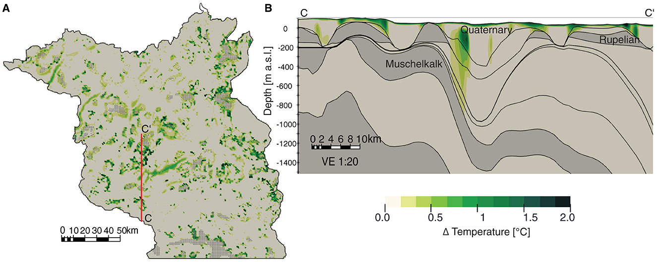
Figure 13. Temperature difference between the first and last 3 years of the transient simulation (1953–1956 and 2011–2014). The plotted data is averaged annually to remove the effect of seasonal fluctuations. (A) Map at 25 m below the surface. Gray dots indicate areas of reduced Quaternary thickness (<25 m). (B) Cross-section; main aquitards are shown in gray.
In Berlin, the most populous city within the model domain, the urban heat island effect due to land use and waste heat adds onto the climatic warming signal, as reflected in the upper boundary condition grids (Figure 3D). The annual mean surface temperature in Berlin has increased during the modeling period by 2°C. After the year 2000, at any month, the temperature in the center of the city is 1–2°C above the Brandenburg average. The warming trend is also reflected in groundwater temperatures: well measurements are indicative of an increase of ~1.5°C in the past three decades (SenStadt, 2020; Supplementary Figure 2). Unlike groundwater level data, groundwater temperature monitoring in Berlin and Brandenburg is sparse, and the depth of the temperature probe relative to the water level in the well is not always documented. This hinders a quantitative comparison of modeled results against the available measurements. This said, though on a more qualitative level, we can note that modeled temperature time series exhibit depth-depended damping of temperature fluctuations, seasonal phase shifts, and a long-term warming trend (Supplementary Figure 2).
Based on a 3D thermo-hydraulic groundwater simulator one-way coupled to a distributed hydrologic model, we have been able to reconstruct the time-dependent pressure and temperature evolution within the sedimentary units in the region of Brandenburg. In this section, we explore model results further with a focus on the relative control that the imposed recharge, the topographic relief, and the heterogenous hydrostratigraphy have on the shallow thermal and pressure fields. Unlike in synthetic box models or 1D analytical solutions, extracting individual effects from our data-driven 3D model is challenging. As shown in the previous section, all driving factors at play, that is the thickness of the Quaternary unit, discontinuities in the Rupelian aquitard, ground steepness and elevation, and net recharge, are quite variable in space (and time). In the following discussion, we aim at discussing these driving forces more systematically and decoupling what can be considered primary and secondary factors controlling flow configuration (4.1), groundwater temperature (4.2), and groundwater level fluctuations (4.3).
We found that hydraulic gradients, acting as the main driver to the groundwater flow in the studied basin, are not exclusively influenced by present-day topographic gradients. Instead, structural dip and stratigraphic layering of geological units and the presence of permeability contrasts and anisotropy all concur to shape the flow in pre-Rupelian aquifers, while recharge variability and anthropogenic groundwater use can be pointed as the sources of hydraulic head and Darcy flux variations in the Quaternary unit.
Several stages of structural deformation and the paleogeographic evolution of the NGB led to a high level of hydrogeological stratification and variable thickness of the stratigraphic formations. This geological heterogeneity is reflected in a relatively complex pressure field and a groundwater system not bounded to individual reservoir units, but characterized by extensive cross-flows and sharp changes in the main flow direction. Regional aquitards (Rupelian, Muschelkalk, and Zechstein) act as hydraulic barriers, responsible for flow reorganization. Vertical flow is more vigorous within steeply dipping strata, adjacent to salt structures or along the southern rim of the basin, and where hydrological windows provide hydraulic communication between otherwise stratigraphically disconnected compartments. The resulting vertical flux has the greatest potential to locally overprint the conductive thermal signature (see also Section 4.2).
The regional flow system in the Buntsandstein and the intermediate flow system, spanning from Keuper to pre-Rupelian Tertiary are not in direct contact with surface waters, with a possible exception of the southern basement uplift, and are dominated by groundwater storage. In these aquifers, groundwater ages are older than the simulated period of six decades and therefore unlikely to be affected by the recent climate variability.
In the Buntsandstein, the deepest modeled aquifer, groundwater flow is controlled by the geometry of the geological units. Indeed, groundwater flows predominantly from south to north/northwest following the regional dip of 1–2°. Consequently, groundwater age also increases from south to north. Inflow of groundwater into the aquifer occurs in the south of Brandenburg, where the Buntsandstein subcrops directly below a thin Quaternary unit due to erosion and non-deposition of the strata in between. This is the only area where we would expect a potential overprinting of the regional flow modulated by long-term climatic variations.
Inflow into the Keuper—pre-Rupelian Tertiary aquifer complex occurs preferentially via leakage from the overlying Quaternary and post-Rupelian Tertiary aquifers. As such, it is genetically connected to two conditions: presence of hydrogeological windows in the Rupelian aquitard and the existence of a hydraulic gradient forcing a downward groundwater flux (Figure 5D). The latter is controlled to a large degree by the present-day topographic relief. Areas where the hydraulic gradient forces upward groundwater fluxes can provide flow paths for outflow of deep Cl−-rich groundwater via hydrogeological windows thereby posing a potential risk of salinization to the drinking-water aquifers. Initial evidence from brackish springs and lakes above the shallow-buried salt domes has been verified by groundwater sampling (Rößling et al., 2010) and modeling (Kaiser et al., 2013; Chabab et al., 2022). At the typical depths of this aquifer complex (>500 m), we did not observe any influence of recharge variability on the groundwater dynamics during the simulation period. However, sustained lower recharge rates over a longer period of time can potentially lead to a pressure decline in freshwater aquifers, and force further brine uprising from saltwater aquifers.
The situation is different if considering the local flow system. In Quaternary and post-Rupelian Tertiary aquifers, groundwater flows inside catchments, from watershed divides toward the drainage network. Those aquifers receive recharge across the upper boundary, either in terms of percolation from the unsaturated zone or due to leakage from incorporated rivers. As a result of the one-way coupling to mHM, recharge occurs in our model where and when the net flux of percolation and baseflow to/from the groundwater storage in mHM is positive. As such, the amount of recharge estimated by mHM only partly follows the actual topography, being principally a function of precipitation, evapotranspiration, soil properties, and land use. As an example, consider the Fläming ridge in SW Brandenburg (Figure 1B). This is the most elevated area in Brandenburg, and yet it does not receive as much recharge as the hills in the NW of Brandenburg, which experience a greater impact of oceanic air masses and receive more precipitation than average (Figure 3C). As a result, the depth to the water table in the south is greater than that in the north, despite a comparable topographic elevation. This leads to different shallow groundwater dynamics than when considering a constant-head boundary condition as a subdued replica of the topography, as usually done in basin-scale groundwater modeling studies. In the latter, recharge is limited to high-elevation areas (highest head) and discharge to low-elevation areas (lowest head), without any consideration of the amount of water effectively reaching the water table.
A gradual and continuous groundwater warming trend as well as the overprint of seasonal fluctuations are strongest in areas of elevated hydraulic head and hydraulic gradients. The factors controlling the penetration depth of the temperature disturbance are imposed groundwater recharge, Darcy flux, and the magnitude of surface temperature variations.
Advective heat transport by groundwater flow can significantly overprint the conductive subsurface temperature field. This is particularly the case beneath recharge and discharge areas, where advective processes depress or increase heat flow, respectively (Ingebritsen et al., 2006). In practice, such deviations in groundwater temperatures profiles from a purely conductive geotherm can be used to estimate vertical water fluxes, and thus present and past recharge rates (Anderson, 2005; Kurylyk et al., 2017). Our initial simulation, that considered constant annual surface temperatures as Type I boundary condition, demonstrates how topographic highs of only a few tens of meters, if sufficient time for equilibration is given, can result in localized negative temperature anomalies throughout the entire sedimentary succession (Figure 12A), with high Peclet numbers pointing to their advective nature (Supplementary Figure 3). However, it is clear that climatic cyclicity and oscillations hinder temperatures in any groundwater system from reaching a true steady state.
In the transient simulation, we have demonstrated that the seasonal groundwater temperature cycling due to conductive heat exchange with the atmosphere is occurring in the upper 20 m and that an additional advective transport component can deepen this feedback. Given that the Quaternary unit is modeled with a homogeneous vertical permeability and a typical thickness >100 m, most of the change is indeed occurring in this unit, with the key factors controlling the depth of the neutral level being the hydraulic gradient, defined either by hydraulic heads or recharge flux, and the magnitude of the annual air temperature variation. Hydrogeological windows in the Rupelian Clay that were thought to play a key role in the vertical advective flow (Noack et al., 2013) cannot trigger this process, but can deepen the thermal front propagation only if the local hydraulic conditions are favorable. In some exceptional cases of very high Darcy flux in the absence of Rupelian aquitard, seasonal temperature fluctuations could reach greater depths, as deep as 100–150 m in our model. The same mechanism is also responsible for the mean increase of ~1.5°C in modeled groundwater temperature from 1953 to present-day in response to the global warming and the urban heat island effect below the city of Berlin, with a modeled anomaly lying within ±0.5°C of the monitored values (Figures 11C, D; Supplementary Figure 2). Additional point sources to the near-surface warming within the study area were attributed to tunnels, underground car parks, and mining operations (Henning and Limberg, 2012; Tissen et al., 2019; Noethen et al., 2023), which have not been incorporated in our model.
Advection-driven undulations of the neutral zone and continuous groundwater warming may impact the state-wide utilization of shallow geothermal heat in Brandenburg, which, as of 2022, consisted of more than 20,000 ground source heat pumps (Ministerium für Wirtschaft, 2023), that, by design, target depths with constant mean annual temperatures.
Despite the lack of modeled heterogeneity in the Quaternary reservoir architecture, and neglecting the details of the hydrodynamics within the unsaturated zone, we have been able to reproduce the seasonal amplitudes of observed groundwater level fluctuations over several decades by properly selecting effective rock properties and considering the assigned net fluxes. However, approximating the multi-annual periodicity and long-term trends with the model has proven to be more challenging.
Modeled groundwater levels predominantly follow the seasonal recharge cycle, showing no delay, with highs during February-March and lows in August-October. Nevertheless, wells characterized by a deeper water table show a smoother and delayed response to recharge pulses (e.g., Well II on Figure 10). We interpret this behavior as an indication of a damped signal from precipitation due to the hydrodynamic dispersion of the advancing wetting front as water infiltrates through a thick unsaturated zone. Indeed, we found such effects to positively correlate with the thickness of the unsaturated zone, becoming increasingly visible for a thickness higher than 10 m. Lischeid et al. (2021), on the basis of principal component analysis of wells and groundwater-fed lakes in Brandenburg, correlated such attenuation to low-frequency patterns in the groundwater time series. Thus, it can be argued that the “deeper” wells are likely to be more suitable to analyze long-term water level trends, since the seasonal signal has been, at least partially, filtered out (Dong et al., 2019; Lischeid and Steidl, 2023).
Inter-annual groundwater level variations in Brandenburg have been attributed to progressive accumulation of soil moisture deficits in the deeper unsaturated zone (Lischeid and Steidl, 2023) or teleconnections between precipitation and the North Atlantic Oscillation (Landesamt für Umwelt Gesundheit und Verbraucherschutz Brandenburg, 2014). mHM recharge fluxes for Brandenburg follow a 5–7-yr periodicity, but in the absence of any damping effect, the seasonal signal is stronger, therefore masking the low-frequency signal in modeled groundwater time series.
In Figure 14 we compare long-term groundwater level trends estimated from a regression analysis, following the procedure described in Länder-Arbeitsgemeinschaft Wasser (2011). The trends based on actual measurements between 1976 and 2013 are presented in accordance with the results from Landesamt für Umwelt Gesundheit und Verbraucherschutz Brandenburg (2014). One caveat of ~37 years of head time series with a single linear regression is evidenced by a reversal in the groundwater trends as seen in some of the wells. For example, the Lausitz mining district underwent a period of mine drainage, followed by mine flooding (Benthaus and Totsche, 2015; Well IV on Figure 10), and the Berlin metropolitan area saw high abstraction rates in the post-war era to supply its growing population and recovering industry, followed by a recovery phase starting from 1990's onward as more sustainable water management strategies were introduced (Frommen and Moss, 2021).
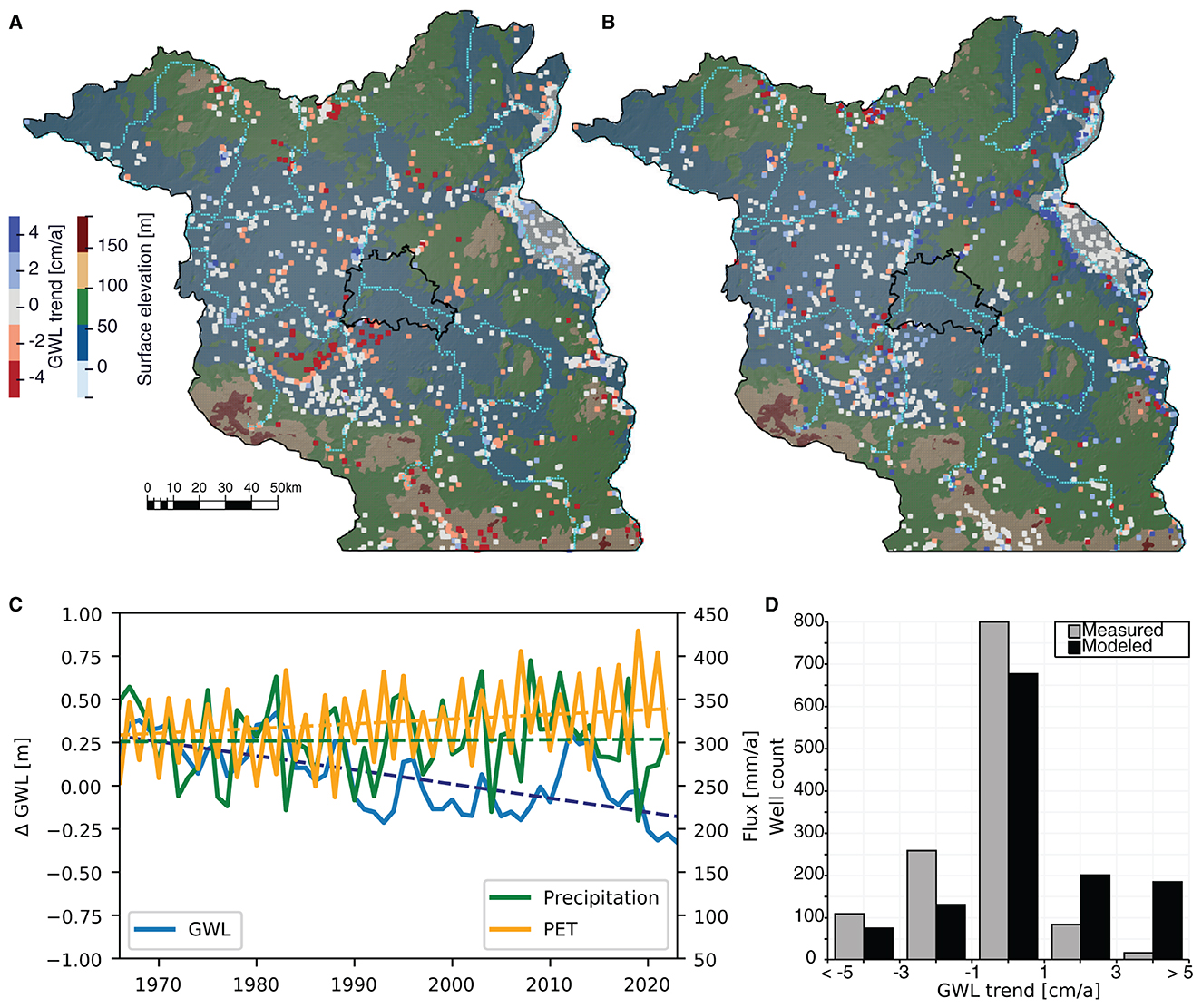
Figure 14. Groundwater level trend (1976–2013). (A) Calculated from well measurements (Landesamt für Umwelt Brandenburg, 2023); (B) Extracted from the model at well locations; (C) annual average hydraulic heads in observation wells in Brandenburg, mHM input fluxes: precipitation and PET; (D) Distribution of modeled and measured groundwater trends.
Despite these assumptions, the majority of wells depicts a decrease in the groundwater level at a rate of 1–3 cm/yr (Figure 14A). Wells with similar behavior are often clustered within a radius of several kilometers. Falling levels are found to correlate spatially with areas where the surface elevation is greater than ~50 m. Highest rate of decline (>10 cm/yr) is found in areas of active or past coal mining in the south of Brandenburg, while lowest values (close to negligible) are seen in the river valleys, occasionally neighbored by wells with rising levels. Falling groundwater levels cannot be directly associated with decline in annual precipitation, which does not exhibit any statistically significant trend (Figure 14C) in the time interval considered. Instead it can be explained by (a) changes in water balance; (b) anthropogenic factors; (c) memory effects in the unsaturated zone.
Regarding the climatic water balance, the observed rise in surface temperatures due to global warming caused an increase of PET in the study area (Figure 14C), which likely led to an increase in the actual evapotranspiration, given no obvious trend in annual precipitation. Coupled groundwater-surface water models from other regions have been able to demonstrate how a higher evapotranspiration can deplete groundwater due to reduced infiltration through the soil and water loss from a shallow-lying water table (Condon et al., 2020).
Local anthropogenic factors depleting groundwater storage in Brandenburg include pumping, coal mine drainage, wetland drainage and other land use changes (Germer et al., 2011). As an evidence, it is typical for neighboring monitoring wells in Brandenburg to show opposing water level trends (Lischeid et al., 2021). Recent high magnitudes of water level decline in local groundwater-fed lakes could only be simulated by superposition of several anthropogenic and natural factors altering the water balance (Somogyvári et al., 2023).
Finally, an apparent monotonic decades-long decline of groundwater levels may arise from memory effects, for example, due to a progressive soil moisture deficit accumulation with depth initiated by a meteorological drought, an effect sometimes referred to as the “drought cascade” (Changnon, 1987; Lischeid and Steidl, 2023).
While inspecting the long-term head behavior based on the model results, we note a higher spatial variability with opposing trends in neighboring grid cells and less clustering than in the observation data (Figure 14B). Clustering can only be seen for wells showing a weak trend (−1 to 1 cm/yr) mostly within lowlands, where the imposed fixed head in the river cells limits the actual rise or fall of groundwater levels. When compared to the observations, the model underestimates the long-term groundwater level decline (Figure 14D). The main explanation is that the net recharge flux derived from mHM does not exhibit a statistically significant trend over time, neither for the entire Brandenburg (Figure 4A), nor in specific locations (Figure 10). Instead, the inflow and outflow components of the groundwater storage in mHM balance each other out on the long-term. Indeed, if we compute the total volume of simulated recharge and discharge over the whole study area for the 1953–2014 period we arrive at an estimate of 2.560e+5 km3 and 2.558e+5 km3, respectively. This results in a cumulative sum of the net recharge fluxes at the scale of individual cells at the end of the simulation to be only −12 to +31 mm. The associated change in groundwater levels would be therefore minimal, that is in the order of few centimeters. Consequently, modeled long-term groundwater level trends are generally weaker than measured ones. This comes back to some inherent limitations of mHM (and of any bucket hydrologic models), that is, in the absence of a deep percolation component, each grid cell of a groundwater reservoir maintains a mass balance between recharge and baseflow over time. Therefore, any single-year increase or decrease of recharge will be compensated by a corresponding baseflow change such that the long-term annual average head will not be significantly affected.
To address these challenges, decoupling cell-based recharge and discharge by lateral redistribution of subsurface water fluxes between grid cells may improve modeling of the long-term groundwater level evolution. On a watershed scale, baseflow routing can be applied to assign Type II boundary condition along river nodes (Jing et al., 2018), but for the Germany-wide mHM model, the routing scheme has not been implemented so far. An alternative could be to assign only positive recharge fluxes from the hydrologic model as a boundary condition while computing the corresponding discharge rates as a function of the hydraulic conductivity, hydraulic gradient, and river network configuration directly in the groundwater model. In such case, a careful calibration of the aquifer parameters becomes crucial to close the water balance.
In addition to input fluxes (precipitation and evapotranspiration), land cover is another transient parameter affecting recharge flux in mHM. Three land cover classes (natural, agricultural, and artificial) are defined for four periods: 1950–1999, 2000–2005, 2006–2011, 2012–2015. Changes in land cover have an immediate impact, resulting in a step-like change of output water fluxes. However, land cover class changes occurred in only 6% of the cells, mostly in the vicinity of Berlin (agricultural to artificial) and in the mining district (natural to artificial; Supplementary Figure 4). Thus, the impact of land cover on the model results is limited.
The uppermost model unit (Quaternary) encompasses three aquifers, all of which are utilized for water supply in Brandenburg, along with corresponding aquitards separating them (Stackebrandt and Manhenke, 2010). In our study, we have approximated this complex architecture of fluvio-glacial deposits characterized by mixed lithologies and abundant discontinuities via unit-averaged effective rock properties, typical for poorly consolidated sand. Recent efforts have been focused on providing a more accurate parameterization of these aquifers, either through higher-resolution structural models (Frick et al., 2019; Chabab et al., 2022) or via stochastic parameter distribution (Truong et al., 2023). The incremental level of heterogeneity in the shallow geology is expected to locally decelerate or enhance surface-to-groundwater interactions.
The sensitivity of the simulation outputs to the mesh resolution was conducted during the FEM mesh set-up. Initially, we carried out test simulations without any vertical refinement, that is the FEM resolution equals the vertical stratification of the input geological model. We found that these runs provided with erroneous output P/T values. In a second stage, we gradually increased the vertical resolution of the numerical mesh until numerically stable and physically consistent (against observations) results were attained. Further mesh refinement is recommended for greater resolution and thus, the accuracy of temperature and Darcy flux profiles in the first tens of meters below the surface, which are sensitive to the high-frequency variations in the upper boundary conditions.
The structural framework of the model does not incorporate faults, which are attributed to basement uplifts, salt diapirism and Pleistocene isostatic adjustment in NGB (Sirocko et al., 2008; Scheck-Wenderoth and Maystrenko, 2013). Some of these faults exhibit significant displacement and a surface expression, however data on faults permeability is not available. Introducing faults would add an extra degree of freedom to the model and can significantly overprint the thermo-hydraulic state at least locally. Previous modeling studies indicated that warm fluids rising along presumably permeable faults can be responsible for a positive anomaly of up to 15°C at a depth of 450 m and a similar magnitude of advective cooling within recharge domains (Cherubini et al., 2014).
Our model does not consider groundwater extraction as an additional sink in the groundwater balance. For a single watershed in Brandenburg (Nuthe), groundwater extraction is estimated to be 8% of groundwater recharge with a total rate of 6 mm/a Landesumweltamt Brandenburg (2009). In Lausitz, the drainage of opencast mines produced a widespread depression in the water levels. Future efforts should characterize such additional fluxes as groundwater extraction, irrigation, riverbank filtration, and lateral inflow/outflow across the model boundaries. Satellite gravimetry may provide an independent, though lower resolution, evidence of groundwater storage reduction in Brandenburg, while multi-scale modeling seems appropriate for evaluating a contribution of the basin-scale flow to the model's water balance A screening analysis suggested that the effect of open vs. closed boundaries on the local groundwater system is minimal since the flow is bounded by smaller-scale catchments and hydraulically connected to the resolved rivers (Figure 5C). The situation differs in regional groundwater system, which showcases an evidence of lateral outflow beyond the model domain (Supplementary Figure 5). However, these boundary effects can be considered of secondary relevance for current study, given that the internal flow geometries within the limits of Brandenburg are not significantly affected by our choice of open vs. closed boundary conditions, and, in principle, in agreement with a flow pattern obtained from the larger-scale model of CEBS (Frick et al., 2022; Supplementary Figure 5).
Our model simulates groundwater flow in a fully saturated domain. Fluxes applied at the top of the model have been derived by one-way coupling the groundwater model to a hydrologic model simulation (mHM) with its own uncertainties and limitations. The mHM setup for Germany used in the present study includes a large number of discharge gauges from upland and headwater regions for model calibration. In contrast, the contribution of pure lowland catchments is rather low and thus limits the performance of the model in lowlands. However, due to the MPR, the effect of parameter changes on the model output is lower in mHM compared to other hydrological models. Simulated fluxes in mHM, like in many other hydrologic models, are calibrated against river discharges but in the majority of the cases not against groundwater levels or other measurements from the subsurface, and are thus subject to uncertainty in soil and rock properties. The travel-time of infiltrating water through the thick unsaturated zone and the delay of recharge pulses are likely to be underestimated.
Given that groundwater accounts for 87.6% of Brandenburg's public water supply and 55.9% of its non-public water supply (Statistisches Bundesamt, 2022), forecasting the system's evolution with respect to climate scenarios becomes crucial for water management. On one hand, climate models suggest an increase in winter precipitation for Brandenburg (GERICS-Climate-Service Center Germany, 2019), which would lead to an overall increased groundwater recharge. On the other hand, rising temperatures will lead to higher evapotranspiration, having an opposite effect on groundwater recharge. Additionally, an increase in the intensity of individual precipitation events may cause a higher surface runoff, further reducing flux through the soil to the water table. Consequently, projecting the trend of groundwater levels due to climate change is challenging, even without considering pumping rates and irrigation. The same applies to groundwater temperatures, which, despite an overall warming trend, may be further altered by advection from evolving recharge rates and their seasonal distribution. Increasing shallow aquifer temperatures might affect groundwater composition, ecosystem, and energy potential, prompting the need for innovative adaptation strategies and heat utilization concepts (Riedel, 2019; Tissen et al., 2019). Present-day subsurface conditions reconstructed by this study can serve as a starting point and input for the next generation of predictive models exploring these effects over longer simulation periods (i.e., 100's−1,000's of years).
In addition to freshwater availability in Quaternary aquifers, climatic impacts on the groundwater dynamics is of relevance for site selection and proper planning and design of geothermal energy utilization concepts as well as in relation to the integrity of subsurface storage projects in saline and brackish formations. In this regard, future work is required to improve current modeling solutions in order to better approximate hydraulic and thermal heterogeneity, and anisotropic conditions in target reservoirs and neighboring aquitards. A use of layer-parallel orientation of Kxy, rather than horizontal, has proven to produce more accurate fluid flow vectors (Poulet et al., 2023). Sensitivity analysis of model parameters, such as permeability, thermal conductivity, and storativity, would become instructive in establishing confidence in model forecasts.
Publicly available datasets were analyzed in this study. Input data for model set-up and output files can be found at: https://dataservices.gfz-potsdam.de/panmetaworks/showshort.php?id=cf5927b9-b491-11ee-967a-4ffbfe06208e.
MT: Conceptualization, Writing – original draft, Data curation, Investigation, Visualization. MC: Software, Writing – review & editing, Conceptualization, Investigation, Supervision. BG: Writing – review & editing, Investigation. AG: Writing – review & editing, Investigation. MS-W: Supervision, Writing – review & editing, Project administration.
The author(s) declare financial support was received for the research, authorship, and/or publication of this article. Funding was provided by Helmholtz Center Potsdam—GFZ German Research Center for Geosciences.
The authors would like to acknowledge Charlotte Krawczyk and Guido Blöcher for their valuable consultations. Additionally, the authors thank Landesamt für Umwelt Brandenburg for kindly providing groundwater temperature data. Constructive suggestions made by two reviewers are greatly appreciated.
The authors declare that the research was conducted in the absence of any commercial or financial relationships that could be construed as a potential conflict of interest.
All claims expressed in this article are solely those of the authors and do not necessarily represent those of their affiliated organizations, or those of the publisher, the editors and the reviewers. Any product that may be evaluated in this article, or claim that may be made by its manufacturer, is not guaranteed or endorsed by the publisher.
The Supplementary Material for this article can be found online at: https://www.frontiersin.org/articles/10.3389/frwa.2024.1353394/full#supplementary-material
Anderson, M. P. (2005). Heat as a ground water tracer. Groundwater 43, 951–968. doi: 10.1111/j.1745-6584.2005.00052.x
Ayachit, U. (2015). The Paraview Guide: a Parallel Visualization Application. Clifton Park, NY: Kitware, Inc.
Benthaus, F. C., and Totsche, O. (2015). The Groundwater Raise in Lignite Mining Induced Areas in Lusetia–Actions Taken to Reduce the Follows Ups. Mining Report (Essen: Bergbau-Verwaltungsgesellschaft mbH), 522530.
Benz, S. A., Bayer, P., and Blum, P. (2017). Global patterns of shallow groundwater temperatures. Environ. Res. Lett. 12:034005. doi: 10.1088/1748-9326/aa5fb0
Bruhn, D. K., Silke, K., Regenspurg, S., and Schumann, F. (2023). Wärmeversorgung in Berlin und Brandenburg durch Geoenergie, Position Paper. Available online at: https://www.gfz-potsdam.de/fileadmin/gfz/sec48/pdf/de/Netzwerke/GEB/Posititionspapier_GEB__2.pdf (accessed December 1, 2023).
Bundesanstalt für Geowissenschaften und Rohstoffeand (2019). Hydrogeologische Karten für den Hydrologischen Atlas von Deutschland.
Bundesanstalt für Geowissenschaften und Rohstoffeand and Staatliche Geologische Dienste (2019). Hydrogeologische Übersichtskarte von Deutschland 1:250.000 (HÜK250). Digitaler Datenbestand, Version 1.0.3. Hannover.
Cacace, M., and Jacquey, A. B. (2017). Flexible parallel implicit modelling of coupled thermal–hydraulic–mechanical processes in fractured rocks. Solid Earth 8, 921–941. doi: 10.5194/se-8-921-2017
Chabab, E., Kühn, M., and Kempka, T. (2022). Upwelling mechanisms of deep saline waters via Quaternary erosion windows considering varying hydrogeological boundary conditions. Adv. Geosci. 58, 47–54. doi: 10.5194/adgeo-58-47-2022
Changnon, S. A. (1987). “Detecting drought conditions in Illinois,” in Circular no. 169 (Champaign, IL: Illinois State Water Survey).
Chen, Z., Grasby, S. E., and Osadetz, K. G. (2004). Relation between climate variability and groundwater levels in the upper carbonate aquifer, southern Manitoba, Canada. J. Hydrol. 290, 43–62. doi: 10.1016/j.jhydrol.2003.11.029
Cherubini, Y., Cacace, M., Scheck-Wenderoth, M., and Noack, V. (2014). Influence of major fault zones on 3-D coupled fluid and heat transport for the Brandenburg region (NE German Basin). Geoth. Energ. Sci. 2, 1–20. doi: 10.5194/gtes-2-1-2014
Condon, L. E., Atchley, A. L., and Maxwell, R. M. (2020). Evapotranspiration depletes groundwater under warming over the contiguous United States. Nat. Commun. 11:873. doi: 10.1038/s41467-020-14688-0
Condon, L. E., and Maxwell, R. M. (2015). Evaluating the relationship between topography and groundwater using outputs from a continental-scale integrated hydrology model. Water Resour. Res. 51, 6602–6621. doi: 10.1002/2014WR016774
Dams, J., Salvadore, E., Van Daele, T., Ntegeka, V., Willems, P., and Batelaan, O. (2012). Spatio-temporal impact of climate change on the groundwater system. Hydrol. Earth Syst. Sci. 16, 1517–1531. doi: 10.5194/hess-16-1517-2012
Deutscher Wetterdienst (2019). Klimareport Brandenburg, 1 Edn. ed. D. Wetterdienst (Deutschland: Offenbach am Main).
Deutscher Wetterdienst—Climate Data Center (2021). Grids of Monthly Averaged Daily Air Temperature (2m) Over Germany, Version v1.0. (Offenbach am Main).
Domenico, P. A., and Schwartz, F. W. (1997). Physical and Chemical Hydrogeology. Hoboken, NJ: John Wiley & Sons, Inc.
Dong, Y., Jiang, C., Suri, M. R., Pee, D., Meng, L., and Rosenberg Goldstein, R. E. (2019). Groundwater level changes with a focus on agricultural areas in the Mid-Atlantic region of the United States, 2002–2016. Environ. Res. 171, 193–203. doi: 10.1016/j.envres.2019.01.004
Förster, A. (2001). Analysis of borehole temperature data in the Northeast German Basin: continuous logs vs. bottom-hole temperatures. Petrol. Geosci. 7, 241–254. doi: 10.1144/petgeo.7.3.241
Franz, M., Barth, G., Zimmermann, J., Budach, I., Nowak, K., and Wolfgramm, M. (2018). Geothermal resources of the North German Basin: exploration strategy, development examples and remaining opportunities in Mesozoic hydrothermal reservoirs. Geolog. Soc. 469, 193–222. doi: 10.1144/SP469.11
Frick, M., Cacace, M., Klemann, V., Tarasov, L., and Scheck-Wenderoth, M. (2022). Hydrogeologic and thermal effects of glaciations on the intracontinental basins in central and Northern Europe. Front. Water 4:818469. doi: 10.3389/frwa.2022.818469
Frick, M., Scheck-Wenderoth, M., Schneider, M., and Cacace, M. (2019). Surface to groundwater interactions beneath the city of Berlin: results from 3D models. Geofluids 2019:4129016. doi: 10.1155/2019/4129016
Frommen, T., and Moss, T. (2021). Pasts and presents of urban socio-hydrogeology: groundwater levels in Berlin, 1870–2020. Water 13:2261. doi: 10.3390/w13162261
Gaupp, R., Moeller, P., Lüders, V., di Primio, R., and Littke, R. (2008). “Fluids in sedimentary basins: an overview,” in Dynamics of Complex Intracontinental Basins: The Central European Basin System, eds. R. Littke, U. Bayer, D. Gajewski, and S. Nelskamp (Berlin: Springer Science & Business Media), 345–366.
Germer, S., Kaiser, K., Bens, O., and Hüttl, R. F. (2011). Water balance changes and responses of ecosystems and society in the Berlin-Brandenburg Region—a review. J. Geogr. Soc. Berlin 142, 65–95.
Goderniaux, P., Brouyère, S., Blenkinsop, S., Burton, A., Fowler, H. J., Orban, P., et al. (2011). Modeling climate change impacts on groundwater resources using transient stochastic climatic scenarios. Water Resour. Res. 47:10082. doi: 10.1029/2010WR010082
Güntner, A., Sharifi, E., Behzadpour, S., Boergens, E., Dahle, C., Darbeheshti, N., et al. (2023). Global Gravity-based Groundwater Product (G3P). V. 1.11. GFZ Data Serv. doi: 10.5880/G3P.2023.001
Haitjema, H. M., and Mitchell-Bruker, S. (2005). Are water tables a subdued replica of the topography? Groundwater 43, 781–786. doi: 10.1111/j.1745-6584.2005.00090.x
Healy, R. W., and Cook, P. G. (2002). Using groundwater levels to estimate recharge. Hydrogeol. J. 10, 91–109. doi: 10.1007/s10040-001-0178-0
Henning, A., and Limberg, A. (2012). Veränderung des oberflächennahen Temperaturfeldes von Berlin durch Klimawandel und Urbanisierung. Brandenburgische Geowiss. Beitr 19, 81–92.
Huenges, E., and Ledru, P. (2011). Geothermal Energy Systems: Exploration, Development, and Utilization. Hoboken, NJ: John Wiley & Sons.
Ingebritsen, S. E., Sanford, W. E., and Neuzil, C. E. (2006). Groundwater in Geologic Processes. Cambridge: Cambridge University Press.
Jing, M., Heße, F., Kumar, R., Wang, W., Fischer, T., Walther, M., et al. (2018). Improved regional-scale groundwater representation by the coupling of the mesoscale Hydrologic Model (mHM v5.7) to the groundwater model OpenGeoSys (OGS). Geosci. Model Dev. 11, 1989–2007. doi: 10.5194/gmd-11-1989-2018
Kaiser, B. O., Cacace, M., and Scheck-Wenderoth, M. (2013). Quaternary channels within the Northeast German Basin and their relevance on double diffusive convective transport processes: constraints from 3-D thermohaline numerical simulations. Geochem. Geophys. Geosyst. 14, 3156–3175. doi: 10.1002/ggge.20192
Kaiser, B. O., Cacace, M., Scheck-Wenderoth, M., and Lewerenz, B. (2011). Characterization of main heat transport processes in the Northeast German Basin: constraints from 3-D numerical models. Geochem. Geophys. Geosyst. 12:3535. doi: 10.1029/2011GC003535
Kestin, J., Sokolov, M., and Wakeham, W. A. (1978). Viscosity of liquid water in the range −8 °C to 150 °C. J Phys. Chem. Ref. Data 7, 941–948. doi: 10.1063/1.555581
Konikow, L. F. (2011). Contribution of global groundwater depletion since 1900 to sea-level rise. Geophys. Res. Lett. 38:48604. doi: 10.1029/2011GL048604
Kumar, R., Samaniego, L., and Attinger, S. (2013). Implications of distributed hydrologic model parameterization on water fluxes at multiple scales and locations. Water Resour. Res. 49, 360–379. doi: 10.1029/2012WR012195
Kurylyk, B. L., Irvine, D. J., Carey, S. K., Briggs, M. A., Werkema, D. D., and Bonham, M. (2017). Heat as a groundwater tracer in shallow and deep heterogeneous media: analytical solution, spreadsheet tool, and field applications. Hydrol. Process. 31, 2648–2661. doi: 10.1002/hyp.11216
Länder-Arbeitsgemeinschaft Wasser (2011). “Fachliche Umsetzung der Richtlinie zum Schutz des Grundwassers vor Verschmutzung und Verschlechterung (2006/118/EG)”, in Teil 5, Bundesweit einheitliche Methode zur Beurteilung des mengenmäßigen Zustands (Sachstandsbericht vom).
Landesamt für Umwelt Brandenburg (2020). Hydroisohypsen und Messwerte des oberen genutzten Grundwasserleiters im Land Brandenburg - Datenserie. Available online at: https://geoportal.brandenburg.de/detailansichtdienst/render?url=https%3A%2F%2Fgeoportal.brandenburg.de%2Fgs-json%2Fxml%3Ffileid%3D2435B954-BA43-4598-B6E1-06AA36F2BAB7 (accessed December 12, 2023).
Landesamt für Umwelt Brandenburg (2022). “Klimawandelmonitoring im Land Brandenburg - Aktualisierungsbericht,” in Fachbeiträge des LfU (Potsdam).
Landesamt für Umwelt Brandenburg (2023). Auskunftsplattform Wasser (APW). Available online at: https://apw.brandenburg.de/ (accessed December 12, 2023).
Landesamt für Umwelt Gesundheit und Verbraucherschutz Brandenburg (2014). “Die Wasserbilanzen der Grundwasserkörper im Land Brandenburg,” in Fachbeiträge des Landesamtes für Umwelt, Gesundheit und Verbraucherschutz ed S. Wieneke (Potsdam), 154.
Lischeid, G., Dannowski, R., Kaiser, K., Nützmann, G., Steidl, J., and Stüve, P. (2021). Inconsistent hydrological trends do not necessarily imply spatially heterogeneous drivers. J. Hydrol. 596:126096. doi: 10.1016/j.jhydrol.2021.126096
Lischeid, G., and Steidl, J. (2023). Why Do Our Models Underestimate Regional Groundwater Trends? Vienna: EGU General Assembly.
Littke, R., Bayer, U., Gajewski, D., and Nelskamp, S. (2008). Dynamics of Complex Intracontinental Basins: the Central European Basin System. Berlin: Springer Science & Business Media.
Magri, F., Bayer, U., Jahnke, C., Clausnitzer, V., Diersch, H., Fuhrman, J., et al. (2005). Fluid-dynamics driving saline water in the North East German Basin. Int. J. Earth Sci. 94, 1056–1069. doi: 10.1007/s00531-005-0497-9
Mather, B., Müller, R. D., O'Neill, C., Beall, A., Vervoort, R. W., and Moresi, L. (2022). Constraining the response of continental-scale groundwater flow to climate change. Sci. Rep. 12:4539. doi: 10.1038/s41598-022-08384-w
Maystrenko, Y., Bayer, U., and Scheck-Wenderoth, M. (2010). Structure and Evolution of the Central European Basin System According to 3D Modeling. DGMK research report (Hamburg) 577-2/2-1, 90.
Ministerium für Wirtschaft Arbeit und Energie Brandenburg. (2023). Geothermie. Available online at: https://mwae.brandenburg.de/de/geothermie/bb1.c.478390.de (accessed December 6, 2023).
NABU-Brandenburg (2021). Wir haben ein Wasserproblem! Available online at: https://nabu-bb.de/wasser-in-brandenburg/ (accessed November 13, 2023).
Noack, V., Scheck-Wenderoth, M., and Cacace, M. (2012). Sensitivity of 3D thermal models to the choice of boundary conditions and thermal properties: a case study for the area of Brandenburg (NE German Basin). Environ. Earth Sci. 67, 1695–1711. doi: 10.1007/s12665-012-1614-2
Noack, V., Scheck-Wenderoth, M., Cacace, M., and Schneider, M. (2013). Influence of fluid flow on the regional thermal field: results from 3D numerical modelling for the area of Brandenburg (North German Basin). Environ. Earth Sci. 70, 3523–3544. doi: 10.1007/s12665-013-2438-4
Noethen, M., Hemmerle, H., Menberg, K., Epting, J., Benz, S. A., Blum, P., et al. (2023). Thermal impact of underground car parks on urban groundwater. Sci. Tot. Environ. 2023:166572. doi: 10.1016/j.scitotenv.2023.166572
Norden, B., Bauer, K., and Krawczyk, C. M. (2023). From pilot knowledge via integrated reservoir characterization to utilization perspectives of deep geothermal reservoirs: the 3D model of Groß Schönebeck (North German Basin). Geothermal Energy 11:1. doi: 10.1186/s40517-022-00242-2
Norden, B., Förster, A., and Balling, N. (2008). Heat flow and lithospheric thermal regime in the Northeast German Basin. Tectonophysics 460, 215–229. doi: 10.1016/j.tecto.2008.08.022
Poulet, T., Sheldon, H. A., Kelka, U., and Behnoudfar, P. (2023). Impact of permeability anisotropy misalignment on flow rates predicted by hydrogeological models. Hydrogeol. J. 31, 2129–2137. doi: 10.1007/s10040-023-02708-4
Rakovec, O., Kumar, R., Mai, J., Cuntz, M., Thober, S., Zink, M., et al. (2016). Multiscale and multivariate evaluation of water fluxes and states over European River Basins. J. Hydrometeorol. 17, 287–307. doi: 10.1175/JHM-D-15-0054.1
Riedel, T. (2019). Temperature-associated changes in groundwater quality. J. Hydrol. 572, 206–212. doi: 10.1016/j.jhydrol.2019.02.059
Rodella, A.-S., Zaveri, E. D., and Bertone, F. M. D. C. (2023). The Hidden Wealth of Nations: The Economics of Groundwater in Times of Climate Change-Executive Summary. Washington, DC: World Bank.
Rößling, H. B., Albrecht, B., Haarring, C., Hermsdorf, A., Herrmann, A., List, U., et al. (2010). Regionale Überblicksdarstellungen und Gebietssteckbriefe. Naturschutz Landschaftpflege Brandenburg. 19, 52–118.
Samaniego, L., Kumar, R., and Attinger, S. (2010). Multiscale parameter regionalization of a grid-based hydrologic model at the mesoscale. Water Resour. Res. 46:7327. doi: 10.1029/2008WR007327
Samaniego, L., Thober, S., Wanders, N., Pan, M., Rakovec, O., Sheffield, J., et al. (2019). Hydrological forecasts and projections for improved decision-making in the water sector in Europe. Bullet. Am. Meteorol. Soc. 100, 2451–2472. doi: 10.1175/BAMS-D-17-0274.1
Scheck, M., and Bayer, U. (1999). Evolution of the Northeast German Basin — inferences from a 3D structural model and subsidence analysis. Tectonophysics 313, 145–169. doi: 10.1016/S0040-1951(99)00194-8
Scheck-Wenderoth, M., and Maystrenko, Y. P. (2013). Deep control on shallow heat in sedimentary basins. Energy Proc. 40, 266–275. doi: 10.1016/j.egypro.2013.08.031
SenStadt (2020). Berlin Environmental Atlas. Berlin: SenStadt, Senate Department for Urban Development, Building and Housing.
Sirocko, F., Reicherter, K., Lehné, R., Hübscher, C., Winsemann, J., and Stackebrandt, W. (2008). “Glaciation, salt and the present landscape,” in Dynamics of Complex Intracontinental Basins. The Central European Basin System, eds R. Littke, U. Bayer, D. Gajewski and S. Nelskamp (Berlin; Heidelberg: Springer), 233–245.
Somogyvári, M., Scherer, D., Bart, F., Fehrenbach, U., Okujeni, A., and Krueger, T. (2023). A hybrid data-driven approach to analyze the drivers of lake level dynamics. EGUsphere 2023, 1–23. doi: 10.5194/egusphere-2023-2111
Stackebrandt, W., and Manhenke, V. (2010). Atlas zur Geologie von Brandenburg im Maßstab 1:1,000,000. Kleinmachnow: Landesamt für Geowissenschaften und Rohstoffe.
Stallman, R. W. (1965). Steady one-dimensional fluid flow in a semi-infinite porous medium with sinusoidal surface temperature. J. Geophys. Res. 70, 2821–2827. doi: 10.1029/JZ070i012p02821
Statistisches Bundesamt (2022). Wasserwirtschaft. Available online at: https://www.destatis.de/DE/Themen/Gesellschaft-Umwelt/Umwelt/Wasserwirtschaft/_inhalt.html#236444 (accessed December 10, 2023).
Szewczyk, J., and Nawrocki, J. (2011). Deep-seated relict permafrost in northeastern Poland. Boreas 40, 385–388. doi: 10.1111/j.1502-3885.2011.00218.x
Taylor, R. G., Scanlon, B., Döll, P., Rodell, M., van Beek, R., Wada, Y., et al. (2013). Ground water and climate change. Nat. Clim. Change 3, 322–329. doi: 10.1038/nclimate1744
Thomas, B. F., and Famiglietti, J. S. (2019). Identifying climate-induced groundwater depletion in GRACE observations. Sci. Rep. 9:4124. doi: 10.1038/s41598-019-40155-y
Tissen, C., Benz, S. A., Menberg, K., Bayer, P., and Blum, P. (2019). Groundwater temperature anomalies in central Europe. Environ. Res. Lett. 14:104012. doi: 10.1088/1748-9326/ab4240
Toth, J. (1963). A theoretical analysis of groundwater flow in small drainage basins. J. Geophys. Res. 68, 4795–4812. doi: 10.1029/JZ068i016p04795
Truong, T. M., Guadagnini, A., and Engelhardt, I. (2023). Characterization of Spatial Heterogeneity of Geomaterials in Large Scale Groundwater Bodies Through a Compositional Data Approach. Vienna: EGU General Assembly.
Werner, A. D., and Simmons, C. T. (2009). Impact of sea-level rise on sea water intrusion in coastal aquifers. Groundwater 47, 197–204. doi: 10.1111/j.1745-6584.2008.00535.x
Wunsch, A., Liesch, T., and Broda, S. (2022). Deep learning shows declining groundwater levels in Germany until 2100 due to climate change. Nat. Commun. 13:1221. doi: 10.1038/s41467-022-28770-2
Keywords: groundwater modeling, climate, groundwater level, geothermal potential, groundwater recharge, mesoscale Hydrological Model (mHM), North German Basin, Brandenburg
Citation: Tsypin M, Cacace M, Guse B, Güntner A and Scheck-Wenderoth M (2024) Modeling the influence of climate on groundwater flow and heat regime in Brandenburg (Germany). Front. Water 6:1353394. doi: 10.3389/frwa.2024.1353394
Received: 10 December 2023; Accepted: 31 January 2024;
Published: 21 February 2024.
Edited by:
Oliver S. Schilling, University of Basel, SwitzerlandReviewed by:
Heather Sheldon, Commonwealth Scientific and Industrial Research Organisation (CSIRO), AustraliaCopyright © 2024 Tsypin, Cacace, Guse, Güntner and Scheck-Wenderoth. This is an open-access article distributed under the terms of the Creative Commons Attribution License (CC BY). The use, distribution or reproduction in other forums is permitted, provided the original author(s) and the copyright owner(s) are credited and that the original publication in this journal is cited, in accordance with accepted academic practice. No use, distribution or reproduction is permitted which does not comply with these terms.
*Correspondence: Mikhail Tsypin, dHN5cGluQGdmei1wb3RzZGFtLmRl
Disclaimer: All claims expressed in this article are solely those of the authors and do not necessarily represent those of their affiliated organizations, or those of the publisher, the editors and the reviewers. Any product that may be evaluated in this article or claim that may be made by its manufacturer is not guaranteed or endorsed by the publisher.
Research integrity at Frontiers
Learn more about the work of our research integrity team to safeguard the quality of each article we publish.