Translating pumping test data into groundwater model parameters: a workflow to reveal aquifer heterogeneities and implications in regional model parameterization

Groundwater modelers frequently grapple with the challenge of integrating aquifer test interpretations into parameters used by regional models. This task is complicated by issues of upscaling, data assimilation, and the need to assign prior probability distributions to numerical model parameters in order to support model predictive uncertainty analysis. To address this, we introduce a new framework that bridges the significant scale differences between aquifer tests and regional models. This framework also accounts for loss of original datasets and the heterogeneous nature of geological media in which aquifer testing often takes place. Using a fine numerical grid, the aquifer test is reproduced in a way that allows stochastic representation of site hydraulic properties at an arbitrary level of complexity. Data space inversion is then used to endow regional model cells with upscaled, aquifer-test-constrained realizations of numerical model properties. An example application demonstrates that assimilation of historical pumping test interpretations in this manner can be done relatively quickly. Furthermore, the assimilation process has the potential to significantly influence the posterior means of decision-pertinent model predictions. However, for the examples that we discuss, posterior predictive uncertainties do not undergo significant reduction. These results highlight the need for further research.

1 Introduction

In this paper we address a problem that is encountered on an almost everyday basis when constructing regional or semi-regional groundwater models. It is how to use estimates of hydraulic properties that are forthcoming from historical interpretation of aquifer tests that have been conducted within a study area, perhaps over a period of many years. These estimates may reside in databases, on paper records, or in old reports.

The quality and type of potentially useable information may vary between tests. For some aquifer tests, drawdown observations may have been taken only in the pumped well. For others, drawdown may have been measured in a number of observation wells. Original drawdown measurements may have been retained in some cases. In others, all that may remain from the test are estimates of transmissivity and storativity that were made through curve matching to analytical pumping test solutions, or straight-line methods such as Cooper-Jacob analysis (Cooper and Jacob, 1946). Some pumping tests may have been of short duration—perhaps a matter of hours. For other tests, pumping may have proceeded for many days. Drawdown recovery measurements may (or may not) be available and may (or may not) have been interpreted. Where drawdown induced by pumping from a single extraction well was measured in multiple observation wells, it is not uncommon for different values of transmissivity and storativity to have been assigned to different pumping-observation well pairs.

Groundwater model parameters are subjected to history-matching using manual or automated methods. These parameters will usually include transmissivity and storativity (Anderson et al., 2015). Ideally, estimates of hydraulic properties that are gleaned from interpretations of aquifer tests that have been conducted in different parts of a model domain should inform the prior probability distributions of model parameters (Neuman, 2003). If the groundwater model is subjected to calibration, this prior probability distribution will feature in regularization constraints that are applied to its parameters as uniqueness is pursued through attainment of a maximum a posterior (MAP) solution to the inverse problem that model calibration poses. Alternatively (or as well), if history-matching employs ensemble-based methods to sample the posterior probability distribution of model parameters, then the prior parameter probability distribution is used to generate initial realizations of parameters; these are then adjusted as regional measurements of system states and fluxes are assimilated (White, 2018).

So the question of how to use estimates of transmissivity and storativity that are forthcoming from historical aquifer tests becomes the question of how these estimates should inform the prior probability distributions of regional model parameters. Embodied in this issue are other issues. These issues include the following:

• The nature of regional model parameterization devices that can best accommodate information derived from historical aquifer test interpretations;

• The level of respect that aquifer-test-interpreted transmissivity and storativity should be afforded as regional model parameters undergo adjustment during history-matching; and

• Determination of the spatial extent of the regional model over which these aquifer-test-derived values should retain influence.

Model parameterization devices vary between models and modelers. The finest scale available for model parameterization is that of individual model cells. Depending on the model, cell dimensions may range from less than a meter to hundreds of meters. For a regional or semi-regional model, it is common for cell dimensions to be in the range of tens to hundreds of meters. There may be some circumstances, therefore, where aquifer-test-inferred hydraulic properties may influence parameters that are attributed to a single model cell, and there may be circumstances where they influence more cells than this. Obviously, the influence of aquifer-test-derived hydraulic properties diminishes with distance from an aquifer test site. At the same time, assessment of an aquifer test's area of parametric influence, must also account for the duration of the test (Leven and Dietrich, 2006). Presumably aquifer tests of longer duration will impact hydraulic properties that are assigned to a greater number of regional model cells.

Aquifer test estimates of transmissivity and storativity obtained through analytical curve matching are solutions to an inverse problem (Kruseman and de Ridder, 1990). Solution of the inverse problem of pumping test data interpretation generally relies on hydraulic property uniformity as its sole regularization device. The uniformity assumption is generally approximate at best. Values that are interpreted for local transmissivity and storativity must therefore compensate for errors in this assumption (White et al., 2014). Their utility in parameterization of a regional model that simulates non-radial groundwater flow, and that acknowledges the presence of aquifer heterogeneity, is therefore questionable. This issue is highlighted when drawdowns observed in different monitoring wells influenced by the same pumping well are interpreted to yield different estimates of transmissivity and storativity. A modeler who intends to make use of information that was forthcoming from the aquifer test generally uses this information to define a range of transmissivity and storativity values which is then used to constrain the prior parameter probability distributions of regional model parameters in the vicinity of the aquifer test. Information on the nature and patterns of local heterogeneity of which these different estimates of transmissivity and storativity speak is generally ignored.

Because hydraulic properties that are inferred from an aquifer test are obtained through solution of an inverse problem, they are both uncertain and correlated with each other. This must be taken into account when assessing the manner in which they should inform parameters of a regional groundwater model.

In attempting to solve problems that are posed by the above issues, we draw inspiration from theories and methods that are employed in the specialist fields of upscaling, pumping-test analysis and data assimilation. We attempt to apply these methods in a way that addresses the practical problem that use of historical aquifer test data poses.

2 Background

2.1 Aquifer test interpretation

In this and following sections of the paper, we use the symbols T and S to refer to estimates of transmissivity and storativity that are obtained from analysis of aquifer test data.

Manewell et al. (2023) show that T and S can be conceived of as complex spatial averages of real-world transmissivity and storativity (which we refer to as T and S) over aquifer material that occupies the vicinity of the test site. This spatial averaging relationship is exact where departures of T and S from their average values are small over the integration domain. However, the linearity relationship that is implied in spatial averaging is less exact where local heterogeneity has a higher amplitude than this.

The kernels (a function that assigns weights to contributions from different spatial locations) of these averaging functions vary with duration of pumping. For a two-well test, they are symmetrical about the line which joins the pumping well to the observation well, and about a line that is perpendicular to this which passes through the mid-point of the wells. In a real-world heterogeneous aquifer, these averaging functions cross hydraulic property boundaries, so that T is sensitive to spatially averaged S and vice versa. “Contamination” of estimates of one hydraulic property by values of the other is not an issue unless the medium in which an aquifer test was conducted is heterogeneous. This is because cross-property kernels of the spatial hydraulic property averaging functions integrate to zero.

The averaging kernel for T as a function of aquifer T grows in area with pumping-test duration. At moderate to large times, contours of constant kernel value are elliptical in shape. The averaging kernel for S as a function of aquifer S has a more complicated shape, with higher values close to the pumping and observation wells. Its contours are increasingly elliptical with distance from the pumping-observation well pair. However, most of its density remains close to these wells.

The implications of these and other aspects of the Manewell et al. (2023) study to representation of pumping-test-inferred estimates of transmissivity and storativity within a groundwater model include the following.

• Unless a pumping test was conducted within the borders of a very large groundwater model cell, the value of T that is inferred from a pumping test is likely to be influenced by the T of aquifer material that occupies a number of neighboring groundwater model cells.

• Aquifer-test-inferred S is likely to be influenced by S of aquifer material that occupies fewer model cells than this.

• In a heterogeneous medium, T is partially reflective of S while S is partially reflective of T of material that occupies one or more groundwater model cells which include and surround the site of an aquifer test.

Repercussions of averaging kernel function details on estimated T and S increase with heterogeneity of the medium in which the aquifer test was undertaken. That is, it increases in inverse proportion to departures from the assumption on which estimates of T and S are based. If hydraulic properties of the tested aquifer are viewed as stochastic variables, then the effects of these averaging kernels on estimated T and S can be conceptualized as dependent on the probability distribution of porous medium hydraulic properties in which the aquifer test takes place.

2.2 Upscaling

The literature on upscaling as an adjunct to simulation of flow in porous media is vast; for an overview, see, for example Karimi-Fard and Durlofsky (2016) and Wang et al. (2023). Like aquifer test interpretation, upscaling solves a kind of inverse problem. It asks what uniform properties should be assigned to an individual model cell so that flow rates and directions across the cell's boundaries are the same as those that result from the heterogeneous medium that the cell actually contains. Some upscaling methodologies that are popular in petroleum reservoir simulation implement direct solution of this inverse problem by populating individual model cells with realizations of small-scale heterogeneity, and then imposing appropriate head/pressure conditions at cell boundaries to calculate resulting flows. Upscaled hydraulic properties are calculated from these (Wen and Chen, 2006; Li et al., 2012; Zhang et al., 2021).

Other upscaling procedures are less precise than this but are more easily implemented. These include methodologies such as harmonic, arithmetic and geometric averaging. Where subsurface media have no clear geostatistical description (which is often the case in groundwater modeling), and/or where subsurface distributions of hydraulic properties are approximately multiGaussian, geometric averaging is often a reasonably good approach to upscaling (Durlofsky, 1992; Wen and Gomez-Hernandez, 1996).

Notionally, estimation of aquifer-test-derived T and S can be considered as a form of upscaling. It imposes a simple set of boundary conditions on a porous medium, and then determines what properties should be assigned to an equivalent homogeneous medium in order to obtain the same drawdown responses at one or a number of measurement points. However, these boundary conditions, and the averaging that is implied by use of these boundary conditions (see above), are very different from those that are used to replace heterogeneity by homogeneity in a rectangular or polygonal cell of a groundwater model. These differences in flow regime, and the averaging functions that they imply, challenge the appropriateness of populating groundwater model cells with pumping-test-derived estimates of T and S.

3 Methodology

3.1 Outline

We first outline an “exact” methodology for utilization of aquifer-test-derived T and S in regional groundwater model parameterization. We then explore ways through which the difficulty and numerical cost of this methodology can be reduced.

Figure 1 shows a pumping well and three observation wells. Let us suppose that these were used for an aquifer test in a fully confined aquifer that was conducted many years ago. Let us further suppose (to make the example easier to visualize) that the three observation wells are separated from the pumping well by a distance of 20 m. All of these wells are presumed to lie within the domain of a regional groundwater model whose cells are 10 m by 10 m (we recognize that these cell dimensions are small compared to those used by most regional models. However, we base our current thought example, as well as the following practical example, on this cell size in order to illustrate how T and S interpreted from an aquifer test may influence more than one model cell. Where regional model cells are large, and where pumping to observation well distances are also large, the same principles apply).

Figure 1

Figure 1. Pumping test configuration and numerical model cells.

Suppose that an old report informs us that the pumping test lasted for 9 h, and that T and S estimates of (T₀), (T₁, S₁), (T₂, S₂), and (T₃, S₃) were made from drawdowns that were measured in the pumping well and in observation wells 1, 2, and 3 respectively. These were estimated using Cooper-Jacob analysis of observed drawdowns. We further suppose that pumping test data are no longer available; only details about pumping rate duration, distances to observation wells and interpreted T and S values remain. From application of the Cooper-Jacob method, we surmise that only “late time” data were used for inference of hydraulic properties; these pertain to times for which drawdown is a linear function of the log of time.

We suppose that spatial variability of T and S at the fine scale are known to be characterized by a variogram whose range, sill and mean value are known (actually a variogram is more likely to characterize the log of these quantities than their native values. This has no effect on the methodology that we now describe).

The first step in implementing this methodology is to use the Theis equation to generate late-time drawdowns in the pumping and observation wells using the four sets of interpreted T and the three sets of interpreted S values. We may generate these at an interval of, say, 10 per decade of time. We then add an appropriate realization of measurement noise to these time series (the choice of noise level is based on local experience in gathering and interpreting pumping test data).

Next, we construct a fine-scale numerical model grid with cell size of 1 m or less that extends to something approaching the limits of pumping-test-induced drawdown (alternatively, it can extend a shorter distance than this from the pumping well if it is equipped with a Dirichlet or Neuman circular boundary condition that is populated under the assumption of hydraulic property uniformity using the geometric average of the above values of T and S). Obviously, this fine model grid will contain many cells.

The aquifer test is simulated by pumping from the central cell of this fine-scale model for 9 h. A cell-to-well correction is required to calculate drawdowns in the pumping well; this can be provided by the CLN package of MODFLOW-USG (Panday et al., 2013) or the MAW package of MODFLOW 6 (Langevin et al., 2017). Using an ensemble Kalman smoother, we then derive (for example) 500 realizations of cell-by-cell T and S that fit aquifer-test-derived drawdowns. These realizations are adjusted from 500 samples of the prior probability distribution of aquifer T and S; as such, they are samples of the posterior (with respect to the aquifer test) joint probability distribution of aquifer T and S. This is a numerically intensive procedure, despite the use of ensemble methods. Its numerical intensity reflects the number of fine-scale model grid cells, and the fact that expression of cell-by-cell hydraulic property variability is likely to impede simulation speed. Nevertheless, methods such as that described by Alzraiee et al. (2022) would (in principle) enable fine-scale posterior T and S fields to be calculated in this way. Note, however, that use of ensemble methods places certain requirement on the prior probability distributions of T and S. These must be multi-Gaussian, or transformable to multi-Gaussian (Evensen et al., 2022).

For each of the 500 samples of the joint posterior probability distribution of fine-scale T and S that are derived in this manner, the geometric average of T and S is evaluated within each cell of the regional model. Under the assumption that geometric averaging is suitable for upscaling fine grid properties to coarse grid properties, we now have 500 samples of the aquifer-test-conditioned, upscaled, regional model parameter field. We can expect that variability of these samples between realizations are less in cells that are closer to the site of the aquifer test than in those that are further from it. Where inter-realization variability is smaller than that which is expected for realizations of prior T and S for the regional model (taking the necessarily upscaled nature of regional model T and S parameters into account), then pumping test measurements have a conditioning effect on regional model parameters. As will be shown below, the conditioning effects of the aquifer test are generally confined to only a few regional model cells that are close to the test site.

Note that the prior probability distribution of cell-based values of T and S used by the regional model can, in principle, be formally calculated from the prior probability distribution of fine-scale T and S. If hydraulic property spatial variability is variogram-based, regional-scale model variograms are easily calculated from fine-scale variograms through spatial averaging (Journel and Huijbregts, 1978). In most cases of practical interest, however, the correlation length and variance of upscaled prior T and S will be guessed. This is because there are rarely sufficient data available to undertake geostatistical analysis. Furthermore, even if they were available, stationarity is unlikely to prevail.

The outcomes of the above process are 500 realizations of aquifer-test-conditioned, upscaled T and S values attributed to regional model cells that are close to the site of the aquifer test. Each such realization is comprised of a map of near-test-site (T_u, S_u)_i pairs; the “u” subscript indicates “upscaled” and the “i” subscript refers to the regional model cell to which a pair of hydraulic properties is assigned. Collectively, these realizations encapsulate the information content of the four (T, S) estimates that emerged from interpretation of drawdowns yielded by the historical pumping test. They account for uncertainties in aquifer test data interpretation that originate from measurement noise on the one hand, and from regularization that was required for unique estimation of four pairs of T and S values on the other hand. Collectively the set of regional-model cell-based (T_u, S_u)_i pairs that populate each of the 500 realizations of (T_u, S_u)_i maps will exhibit correlation between T_ui and S_ui values ascribed to neighboring model cells; values of T_ui and S_ui within each model cell will also be correlated.

Optimal usage of the 500 realizations of test-site-proximal maps of upscaled T_ui and S_ui that are obtained in this manner depends on the parameterization scheme that is adopted by the regional model. Suppose, for the moment, that history-matching of this model is also based on ensembles of cell-by-cell parameter values. In accordance with the operation of ensemble Kalman methods, samples of the prior regional model parameter probability distribution are adjusted until they sample the posterior parameter probability distribution as measurements of system state and flux that comprise the history-matching dataset of the regional model are assimilated. The 500 realizations of near-test-site (T_u, S_u)_i samples that were obtained in the manner described above can therefore be used to condition 500 realizations of prior regional model parameter fields that are used to initiate the regional model history-matching process. Conditioning of cell-by-cell property fields is easily undertaken if these fields are generated using the sequential Gaussian methodology; see, for example, Deutsch and Journel (1997).

Stochastic (T_u, S_u)_i maps that surround other historical aquifer test sites can be obtained in a similar manner. These too can be part of the spatial conditioning dataset of prior realizations of regional model parameters.

3.2 Issues

The methodology that is described above is “conceptually correct” except, perhaps, for its use of geometric averaging as an upscaling device from fine-scale model cells to regional-scale model cells. However, this approximation can be justified by the numerical cost of implementing a more rigorous upscaling methodology, and by the fact that deployment of a more exact upscaling device requires an appropriate geostatistical descriptor for fine scale hydraulic properties. Ideally, the same descriptor could be used for upscaling as that which is used to generate prior realizations of fine-scale model parameters that form the basis for aquifer test data re-interpretation in the manner described above. However, in groundwater modeling contexts, geostatistical characterization of subsurface media is approximate at best and unreliable at worst. Use of geometric averaging for upscaling purposes must be seen in this perspective.

Vagueness of stochastic characterization of real-world hydraulic properties is a matter of concern, not just for upscaling to regional model cells, but also as a fundamental element of ensemble-based aquifer test data assimilation. Nevertheless, adoption of a fine-scale hydraulic property prior is something that cannot be avoided for either of these operations. The methodology described above places heavy reliance on use of a (generally multi-Gaussian) prior hydraulic property distribution that yields hydraulic property realizations that still respect the prior after history-match adjustment; this is a requirement of ensemble-based history-matching. This precludes use of a prior that may express more realistic representations of fine scale hydraulic property detail. It also mandates use of a prior which may be itself uncertain and whose uncertainty is not respected in the data assimilation process. This is a weakness of the methodology.

Another problem with the methodology that is outlined above is its high numerical cost. The fine model grid that is used for aquifer-test re-interpretation, and the iterative nature of ensemble-based data assimilation, impose a considerable computational burden. Use of “hierarchical methods” that acknowledge uncertainty in the prior probability distribution of subsurface hydraulic properties is likely to increase this burden considerably (Oliver, 2022).

3.3 Data space inversion

“Data space inversion” (DSI) refers to a class of ensemble methods that supports direct conditioning of model predictions by measurements of past system behavior without the need to adjust model parameters. This can overcome some of the problems that are discussed above. We briefly describe the theory on which it is based, while referring readers to papers such as Lima et al. (2020) and Delottier et al. (2023) for further details.

We use the vector h to designate a set of observations of system behavior. Collectively, these comprise a history-matching dataset. Let the vector o denote model-calculated counterparts to measurements comprising h. Meanwhile, the vector s encapsulates model predictions that are of interest to us. In the present case, these predictions are geometric averages of aquifer-test-conditioned fine-scale hydraulic properties over regional model cells.

The first step in the application of DSI is the generation of stochastic fields at the fine model scale, similarly to the method described previously. A significant difference with the previously described methodology, however, is that these parameter fields are not history-match adjusted. Hence, they can be of arbitrary complexity and can express arbitrary hydraulic property detail. For example, they may include categorical features such as faults or geological boundaries whose positions may change between realizations. Alternatively, or as well, they can include a high degree of non-stationarity that allows spatial correlation and orientation of hydraulic property connectedness to vary in different parts of the aquifer test drawdown cone. Non-stationary cell-by-cell parameter fields are easily generated using the moving average method described by Oliver (1995) and adapted for non-stationarity by Higdon et al. (1999), Paciorek and Schervish (2006), and others. Public-domain packages which implement non-stationary stochastic field generation are readily available; see, for example, Doherty (2023a,b). Additionally, there is no reason why different realizations that comprise the prior hydraulic property ensemble cannot be generated using different prior hydraulic property distributions. The resulting ensemble of hydraulic property fields can therefore accommodate limitations in a modeler's ability to stochastically characterize spatial variability of local hydraulic properties.

Each one of these hydraulic property fields (let us again assume that there are 500 of them) is then used to calculate the geometric average of T and S in regional model cells whose properties may be informed by the aquifer test. These upscaled (T_u, S_u)_i pairs comprise the vector of predictions s made by the statistical model (actually, we work with the natural logs of these quantities, as the hydraulic property inference problem then becomes more linear).

The pumping test is then simulated using each of the 500 hydraulic property fields. Model-outputs o corresponding to h are thereby generated. On the basis of these 500 model run outcomes, standard statistical formulas can be used to calculate the means of both s and o; this is the vector $\left[\begin{array}{c}\underset{\_}{s}\\ \underset{\_}{o}\end{array}\right]$. A covariance matrix that links s and o is just as easily evaluated. We symbolize this as $C\left(\left[\begin{array}{c}\text{s}\\ \text{o}\end{array}\right]\right)$(actually, the methodology often performs better if the elements of s and o are histogram-transformed prior to construction of these empirical statistical quantities; see Jiang et al. (2021). We adopt this approach in the example presented below but discuss it no further here in order to maintain simplicity of the discussion).

Next, a surrogate statistical model (SSM) is constructed that links o and s. It is formulated as follows.

$\begin{array}{ll}\left[\begin{array}{c}s\\ o\end{array}\right]=\left[\begin{array}{c}\underset{\_}{s}\\ \underset{\_}{o}\end{array}\right]+C^{1/2}\left(\left[\begin{array}{c}s\\ o\end{array}\right]\right)x& (1)\end{array}$

$C^{1/2}\left(\left[\begin{array}{c}\text{s}\\ \text{o}\end{array}\right]\right)$ is derived by subjecting the above-mentioned empirical $C\left(\left[\begin{array}{c}\text{s}\\ \text{o}\end{array}\right]\right)$matrix to singular value decomposition, taking the square root of singular values, and then re-assembling the matrix. In the example discussed below, we retain 0.999 of total singular value energy in formulation of the final matrix. It is easily established that statistical relationships between s and o that are embodied in Equation 1 are the same as those that characterize the outputs of the complex model which it replaces, provided that the parameters of the statistical model (the individual elements of x in Equation 1) are independently normally distributed.

Once the model of Equation 1 has been formulated, the next step is to condition predictions s by measurements h. This is done by subjecting this surrogate model to Bayesian history-matching. In our example we use the PESTPP-IES iterative ensemble smoother (White, 2018). This yields posterior samples of statistical model parameters x which can then be used to generate posterior samples of s. Because the surrogate model of Equation 1 runs in a fraction of a second, conditioning of s by h is a numerically trivial exercise. The outcome of the conditioning process is an ensemble of 500 maps of aquifer-test proximal (T_u, S_u)_i. These can be used to condition 500 realizations of regional model parameters in the manner described above.

We now demonstrate the above methodology using a synthetic test case. We then discuss ways in which the methodology can be modified for easier use in real-world settings. In the example that we present below, we do not avail ourselves of the opportunity to use a categorical or non-stationary prior probability distribution for fine scale T and S. Furthermore, the prior parameter probability distribution that we adopt for regional model parameters is directly upscaled from the fine scale prior. These controlled conditions support a systematic assessment of the methodology. Figure 2 shows the steps required to achieve this.

Figure 2

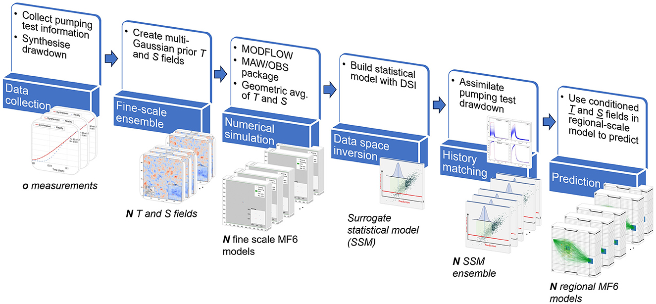
Figure 2. Schematic that shows the steps required to assimilate drawdown data to condition regional-scale model cells.

4 An example

For this study, we continue to discuss the example of Figure 1.

At first we assume that hydraulic testing was undertaken several decades ago. The aquifer is confined. Its mean transmissivity is thought to be 100 m²/day while its mean storativity is thought to be 0.001. Hydraulic property measurements from tests conducted across the aquifer elsewhere exhibit a standard deviation of 0.8 for both T and S on the natural log scale.

A hydrogeologist conducted a 9-h pumping test. Drawdown and recovery were recorded in the pumping well and in three adjacent monitoring wells. The pumping well had a diameter of 15 cm. Hydraulic property estimation relied on the Cooper-Jacob straight-line method applied to late-time drawdown data. Interpreted T and S were summarized in a brief report as shown in Table 1. Unfortunately, drawdown measurements were not included in the report and are absent from project archive databases.

Table 1

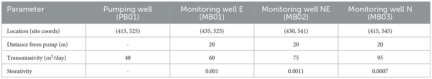
Table 1. Pumping test interpretation presented in historical report.

To begin the workflow described above, we use the interpreted T and S values and the Theis equation to synthesize drawdowns in all observation wells. These are represented by the red points in Figure 3. In keeping with the manner in which data were originally interpreted, we exclude the first decade of these data when re-inferring aquifer transmissivity and storativity, thereby retaining only the linear part of these drawdown curves.

Figure 3

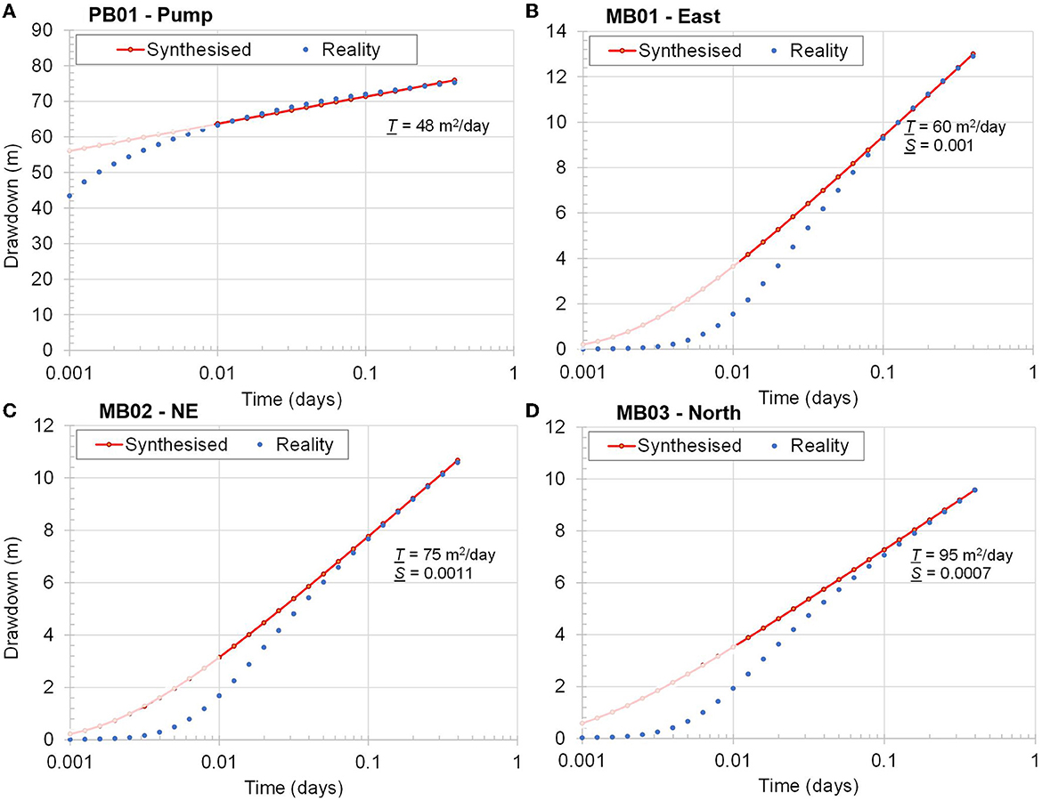
Figure 3. Theis synthesized drawdowns compared to “real” drawdowns at four monitoring locations. T and S values estimated from late-time drawdowns are also shown in this figure. (A) PB01-Pump. (B) MB01-East. (C) MB02-NE. (D) MB03-North.

For the sake of comparison, we also assume that drawdown measurements from this pumping test were eventually discovered. The aquifer parameters for this synthetic example are thereby assumed to be calculated from the blue points shown in Figure 3. Well bore storage effects and hydraulic heterogeneity explain perturbations of these points from those calculated using the Theis equation. This effect is readily included in our small-scale model. We assume that a suite of recovery measurements were also discovered, these spanning a period of 48 h.

An exponential semi-variogram with a range of 100 m and a natural log standard deviation of 0.8 was used to characterize T and S stochasticity over a 1 m grid spanning 1,000 × 1,000 m (we assume that this simplistic characterization of site heterogeneity is in accordance with prevailing site concepts. We note, however, that the methodology described in this paper requires assumptions of neither stationarity nor continuity of hydraulic property fields). This fine scale model therefore has 1,000,000 cells. Five hundred and one realizations of T and S fields were generated; one of these was selected as “synthetic reality.” The blue drawdown measurements depicted in Figure 3 were generated from this “reality.”

The pumping test is simulated using a two-dimensional MODFLOW 6 model. The Multi Aquifer Well (MAW) package is used for extraction of water from the local aquifer; this accounts for well bore storage and losses and performs the necessary cell-to-well correction. In accordance with pumping test specifications that were provided in the report, we simulate extraction at a rate of 2,000 m³/day for 9 h. We also simulate 48 h of recovery.

The eastern and western boundaries of the model domain are no-flow while the northern and southern boundary conditions are Dirichlet. These impose a north-to-south hydraulic gradient of 0.005 on hydraulic heads. These boundary conditions do not affect aquifer test drawdown measurements because drawdowns do not extend to aquifer boundaries. However, as a matter of convenience, they are the same as those used by the regional model for which upscaled parameters are required (see Figure 4A).

Figure 4

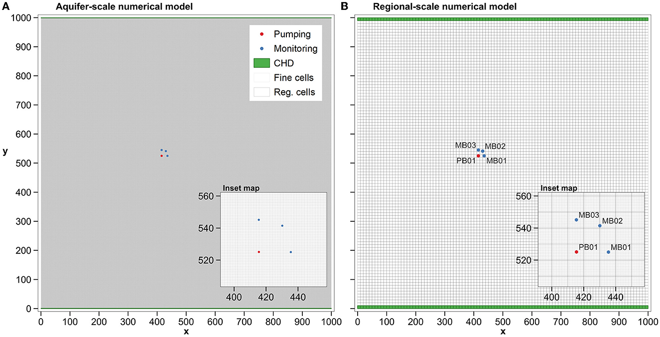
Figure 4. (A) Aquifer-scale (i.e., fine) model grid, together with locations of pumping well, observation wells and boundary conditions. (B) Regional-scale model grid and boundary conditions.

We evaluate the method using a number of different subsets of the full synthetic observation dataset. This allows us to document the performance of the methodology that we describe above, while also illustrating the worth of information residing in aquifer test data that is often ignored. At first we use only synthesized drawdown measurements from the pumping well itself over a time span from 0.01 days to 9 h. The synthetic dataset is then expanded to include synthesized drawdown measurements from one, and then two, offset monitoring wells. This illustrates improvements in the ability of aquifer test data to condition regional model parameter fields when drawdown measurements in one or more observation wells are available. Finally, we use all drawdown and recovery data from the pumping and three observation wells to condition the regional model parameter field.

The regional scale model is depicted in Figure 4B. With grid cell lengths of 10 × 10 m the grid is comprised of 10,000 model cells. Each cell of the regional model therefore contains 100 cells of the fine model. We suppose that the regional model was built to predict particle trajectories and drawdowns toward a planned excavation in the central region of the model domain. This is further discussed below.

The left part of Figure 5 shows “synthetic reality” T and S fields over the domain of both models. Note that transmissivities near the pumping test site are significantly lower (around 30 m²/day) than the average value of 100 m²/day used for generating this field. Note also the presence of elevated storativity to the southeast of the aquifer test site.

Figure 5

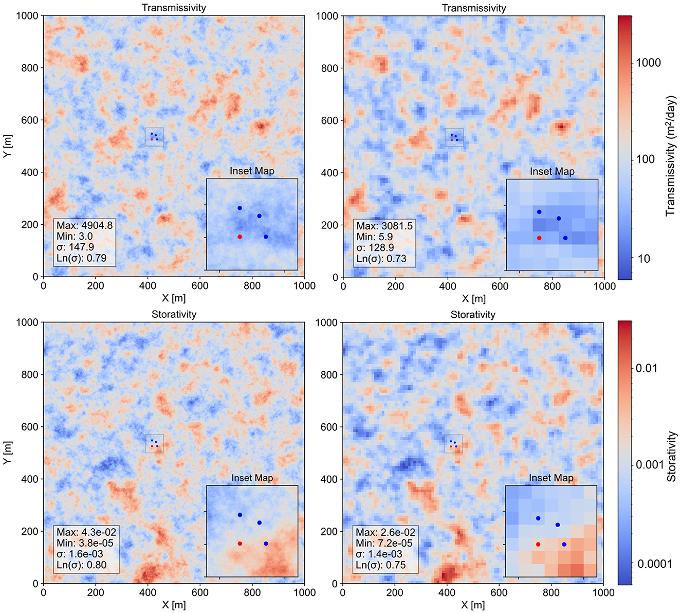
Figure 5. The left part of this figure shows fine-scale reality T and S fields. The right part of the figure shows T_ui and S_ui fields for the regional model derived through geometric upscaling of the fine scale field.

The right part of Figure 5 shows upscaled reality T and S fields for the regional model. Upscaling is performed by geometrical averaging of fine-scale T and S fields within each regional model cell. To validate the integrity of this method of upscaling, flows across all faces of all regional model cells were compared with summed flows across the boundaries of fine model cells that coincide with all of these coarse model cell boundaries. Excluding cells proximate to the pumping well, the maximum flow discrepancy was commensurate with errors incurred in the numerical model solution process.

4.1 Aquifer-test-constrained upscaling using drawdowns from pumping well

At first, we apply the above methodology to drawdowns that are measured in the pumping well only. Figure 6 presents a map of the mean upscaled (T_u, S_u)_i parameter field for that part of the regional model that surrounds the aquifer test site. This is compared with T and S fields obtained from geometric upscaling of real parameters fields (see the left side of Figure 6). Samples of the posterior probability distribution of T_ui and S_ui at selected regional model cells are also shown, together with samples of the prior probability distribution of T_ui and S_ui, together with the true values of T and S in these cells. The latter samples are obtained by geometric upscaling of the 500 parameter fields that were used for construction of the DSI model. These figures demonstrate that drawdown measurements from a single pumping well taken over a limited time do appear to provide some insights into transmissivity in the vicinity of the test site. The low values of T that prevail in this area are reflected in the mean upscaled T_ui field; they are also reflective of the T value of 48 m²/day interpreted from pumping-well drawdown data. In addition to this, the T histogram plot exhibits a shift in the direction of lower transmissivity, despite the fact that uncertainty of T is not reduced by much.

Figure 6

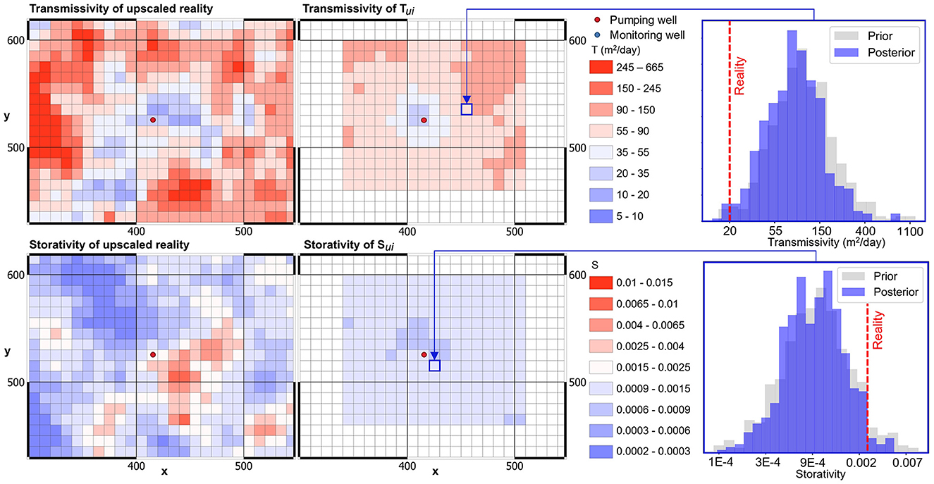
Figure 6. “Real” and pumping-test-constrained mean (T_u, S_u)_i fields are compared on the left. Prior and posterior distributions of upscaled T_ui and S_ui are compared for two model cells on the right.

Prior and posterior standard deviations of T_ui and S_ui (actually their natural logs) can be calculated from prior and posterior realizations of (T_u, S_u)_i. From these it is a simple matter to map relative reduction in standard deviation of T_ui and S_ui accrued through conditioning by drawdown measurements; see Figure 7. The maps presented in this figure indicate that the uncertainty of T_ui is reduced by 78% in the immediate vicinity of the pumping well. As expected, and as is indicated by the spatial averaging function presented in Manewell et al. (2023), information forthcoming from late-time pumping well drawdowns does not significantly reduce the uncertainty of S_ui.

Figure 7

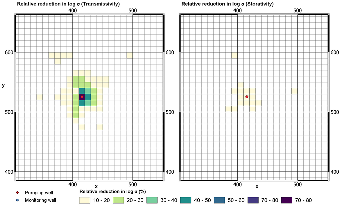
Figure 7. Relative reduction in posterior log standard deviation of T_ui (left) and S_ui (right) accrued through assimilation of late-time drawdowns in pumping well.

4.2 Aquifer-test-constrained upscaling using drawdowns from one observation well

We now repeat the above numerical experiment, this time using Theis-equation-synthesized measurements separately from each of the northern (MB03) and eastern (MB01) observation wells. Figure 8 shows that when drawdown data from MB1 are used to produce maps of (T_u, S_u)_i, the mean T_ui decreases across a wide area; it aligns with the Cooper-Jacob estimated value of 60 m²/day based on drawdowns from this well. In contrast, when drawdown data from MB03 is used to produce maps of (T_u, S_u)_i, the mean T_ui are higher than this; this mirrors the historical estimate of 95 m²/day derived from Cooper-Jacob interpretation of late drawdown data in this well. However, drawdowns from neither test resolve details in the structure of the real T and S fields.

Figure 8

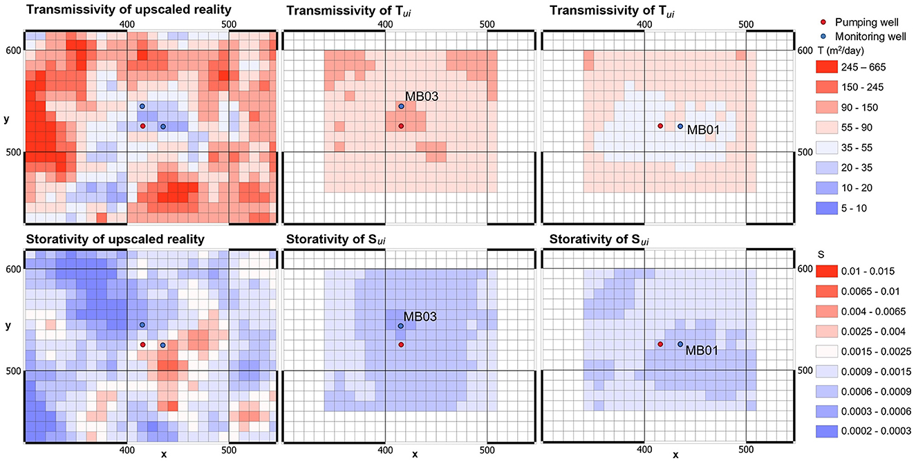
Figure 8. “Real” and pumping-test-constrained mean (T_u, S_u)_i fields are compared. Late time drawdowns in a single observation well are used to constrain (T_u, S_u)_i. The single well is shown in respective figures.

Figure 9 depicts relative uncertainty reduction. This figure illustrates that the posterior uncertainties of T_ui and S_ui are reduced over a wider area than when drawdowns from only the pumping well are used to estimate aquifer properties. However, the relative reduction in the standard deviation of individual T_ui values is of lower magnitude, peaking at around 38%.

Figure 9

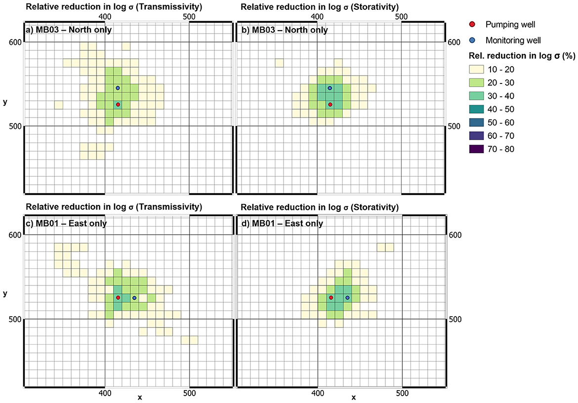
Figure 9. Relative reduction in posterior log standard deviation of T_ui (left) and S_ui (right) accrued through assimilation of late-time drawdowns in individual observation wells. (A, B) MB03-north only. (C, D) MB01-east only.

4.3 Aquifer-test-constrained upscaling using drawdowns from two observation wells

We now derive maps of aquifer-test-constrained (T_u, S_u)_i under the assumption that historical drawdowns from two observation wells (i.e., MB01 and MB03) were used to historically interpret T and S, and that individual values of T and S obtained from interpretation of each well-specific set of drawdowns were recorded in the historical report. In accordance with the workflow described above, we use the Theis equation to generate two sets of observation-well-specific drawdowns. Then, using data space inversion, we produce a single posterior ensemble of 500 sets of (T_u, S_u)_i maps from which posterior statistics of T_ui and S_ui can be calculated.

Figure 10 maps mean T_ui and S_ui obtained through this process; these maps are compared with the real T_ui and S_ui. It is apparent from these maps that simultaneous re-interpretation of synthetic high-time drawdowns that are derived from the two, separate, historical estimates of T and S yields a high level of resolution for subsurface hydraulic property structure. The patterns of T_ui and S_ui heterogeneity that emerge from this process resemble patterns that occur in reality. Furthermore, inferred mean T_ui and S_ui values near the test site are well-aligned with true values. T_ui is particularly well-resolved on the outside lobes of the well-configuration.

Figure 10

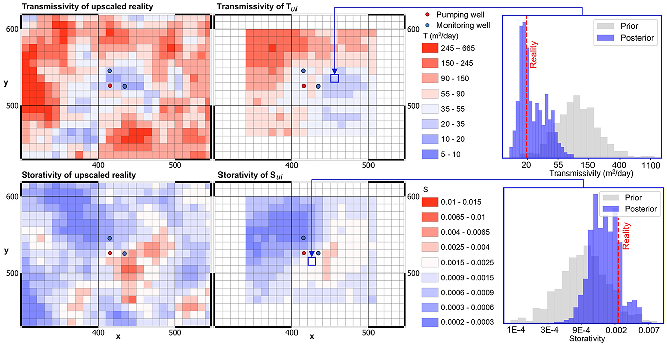
Figure 10. “Real” and pumping-test-constrained mean (T_u, S_u)_i fields are compared. Late time drawdowns in two observation wells are used to constrain (T_u, S_u)_i. Prior and posterior distributions of T and S are compared for two model cells on the right.

Figure 11 reveals that the posterior uncertainty of aquifer-test-constrained T_ui and S_ui decreases across a wider area when drawdowns from two wells are simultaneously reinterpreted than for when drawdown from a single well is reinterpreted. Relative reduction of S_ui peaks at 44%.

Figure 11

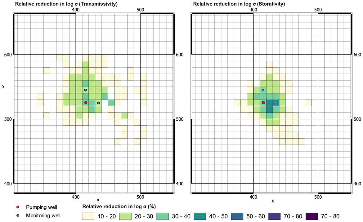
Figure 11. Relative reduction in posterior standard deviation of T_ui (left) and S_ui (right) accrued through simultaneous assimilation of late-time drawdowns in two observation wells.

4.4 Aquifer-test-constrained upscaling using all drawdown and recovery data

As stated above, our final numerical experiment utilizes the “recently discovered” original set of field-observed drawdown and recovery data over a 48-h period. Use of the original drawdown data allows us to base our upscaling workflow on actual drawdown measurements instead of relying on Theis-synthesized data. We also assume that data rediscovery has given us access to supplemental information in the form of groundwater flow rates into the pumping well-provided by in-line flow meter records.

To demonstrate worth of early-time, late-time, recovery, and flow data components of the rediscovered dataset, we repeat the upscaling process multiple times. On each occasion we introduce a new component of aquifer test data to the workflow. Figure 12 provides maps of relative reduction of T_ui and S_ui as more historical data are introduced to the workflow. Measurement data from the pumping well and three observation wells are used in production of all of these plots.

Figure 12

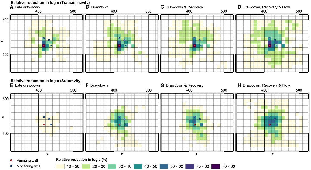
Figure 12. Relative uncertainty reduction of upscaled transmissivity and storativity as extra data are added to the (T_u, S_u)_i estimation workflow. Hydraulic property estimation is based on measurements in the pumping well and in three observation wells. (A, E) Late drawdown. (B, F) Drawdown. (C, G) Drawdown and recovery. (D, H) Drawdown, recovery, and flow.

In accordance with results that have already been presented, Figure 12 demonstrates that use of late-time drawdowns alone (which is equivalent to Cooper-Jacob interpretation) offers limited insights into the heterogeneity and uncertainty of S_ui. In contrast, simultaneous use of all drawdown data reduces the uncertainty of upscaled storativity; the addition or recovery data shines further light on the magnitude and disposition of subsurface S_ui. Interestingly, the addition of well-entrant flows to the aquifer test data reinterpretation process appears to have a significant effect on the uncertainties of both T_ui and S_ui. Maximum absolute uncertainty reduction for these is now 80 and 56%, respectively. At the same time, the area over which uncertainty reduction is experienced is dramatically increased.

Figure 13 shows mean (T_u, S_u)_i parameter fields calculated using the above-described workflow where all components of drawdown and recovery data from all wells are included in the data re-interpretation process. The resolution of upscaled transmissivity and storativity in the vicinity of the pumping test site that is afforded by re-interpretation of these data is marked.

Figure 13

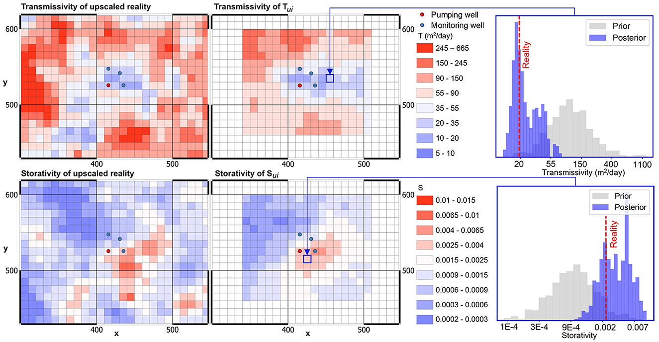
Figure 13. “Real” and pumping-test-constrained mean (T_u, S_u)_i fields are compared. Drawdowns, recoveries and borehole-entrant flow from the original pumping test are re-analyzed. Prior and posterior histograms of T_ui and S_ui are shown for two different regional model cells on the right.

4.5 A regional model prediction

We now deploy the regional model. Two predictions are made using this model. Our intention is to examine how conditioning of the model's parameter field using the workflow discussed above affects the values and uncertainties of these predictions. The predictions are affected by a large volume of aquifer that is close to the location of the historic pumping test. We use the full set of data that were gathered during the historical pumping test. Recall that these are comprised of drawdowns and recoveries in the pumping well and three observation wells, together with flow into the pumping well.

We consider that a proposal has been made to excavate through the entirety of the aquifer at the south-east of the study site. These excavations will reduce the water table by about 100 m. Excavation is simulated through emplacement of a MODFLOW 6 drain boundary condition at the excavation site. Excavation to the maximum depth is considered to be instantaneous. As part of an environmental impact study, the regional-scale model is required to calculate drawdowns induced by this excavation. Also of interest are travel times of a contaminant of interest across the aquifer test site toward the pit. To explore this issue, a single particle is released at the moment of pit excavation; the time taken for this particle to terminate its trajectory at the pit is the prediction of interest.

Figure 14 compares prior and posterior particle paths across the study area from the same release point at the left of the aquifer test site. These are calculated using MODPATH 7 (Pollock, 2016); porosity is assumed to be 0.1 and spatially uniform. Prior particle paths are calculated using prior upscaled (T_u, S_u)_i fields. Recall that these are obtained by geometric averaging of the 500 prior fine-scale T and S fields that were used for construction of the DSI model. Posterior (T_u, S_u)_i fields are the same as prior fields except in the immediate vicinity of the test site where they are conditioned by aquifer test data using the methodology described above. Figure 14 suggests a mild narrowing of the posterior probability distribution of particle trajectories accrued through aquifer test data conditioning. However, the mildness of this narrowing is noteworthy. Diversity of particle paths is affected by the presence (of otherwise) of areas of low transmissivity within the subsurface, as groundwater must flow around these areas. The existence of this area has been exposed by aquifer test data re-interpretation.

Figure 14

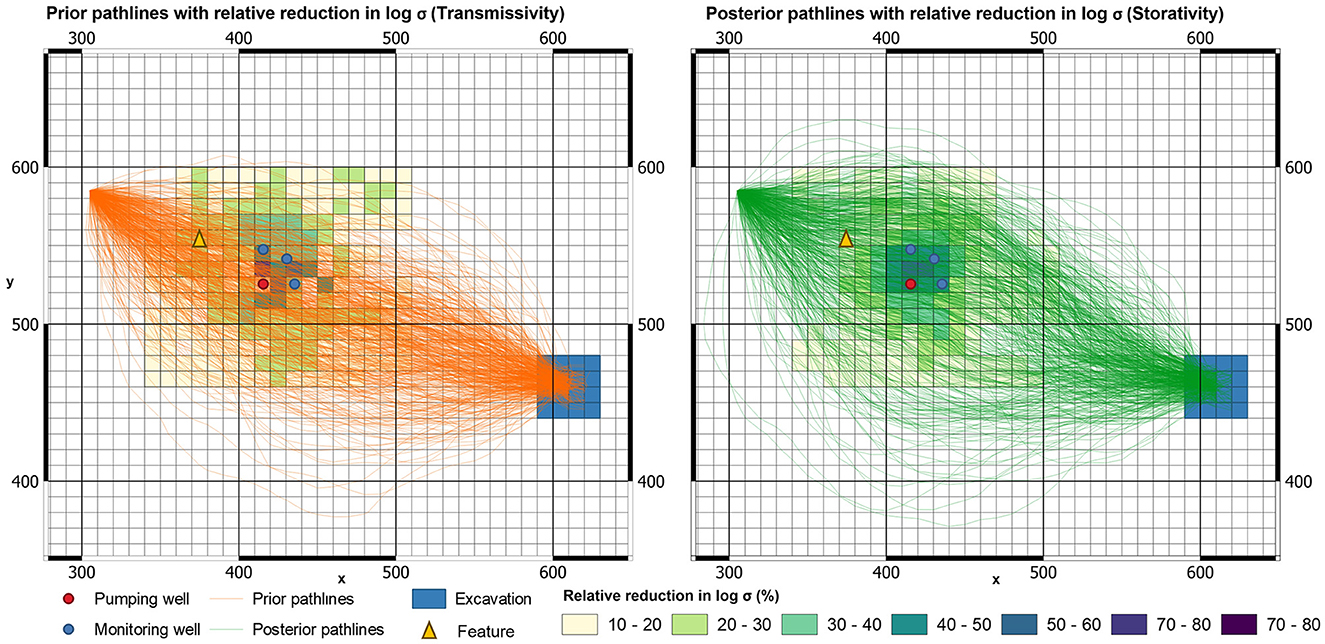
Figure 14. Prior (left) and posterior (right) single particle travel paths from 500 realizations. These are underlain by a map of relative reduction of posterior standard deviation.

The first of the two predictions on which we focus are the particle travel time to the excavation site. The second is excavation-incurred drawdown at a feature to the west of the aquifer test site after 30 years of excavation. The prior and posterior probability distributions of these predictions are depicted in Figure 15. It is apparent from these plots that the posterior medians of both of the particle travel time prediction and the drawdown prediction are lower than the prior medians of these predictions. The lower median drawdown may reflect lower transmissivities that are inferred in the vicinity of the point of interest. The faster median particle travel time may reflect a shortening of the mean particle travel path. What is noteworthy, however, is that the uncertainties of neither of these predictions are reduced by much.

Figure 15

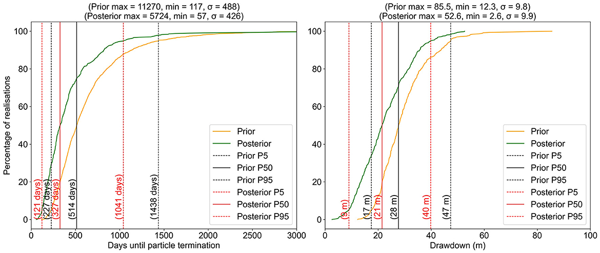
Figure 15. Cumulative exceedance statistics of particle travel time (left) and drawdown (right).

The above analysis was repeated for the most data-poor of our analyses, this being the case for which high-time pumping well drawdowns alone are used for regional model (T_u, S_u)_i conditioning. In this case prior and posterior uncertainties are almost identical. However, the analysis yielded a similar reduction in median posterior drawdown (a shift of 5 m for this data-poor case vs. 7 m for the data rich case). However, it yielded a smaller reduction in median particle travel time (128 days for the data-poor case vs. 287 days for the data-rich case).

5 Discussion

The methodology whose concepts are presented in earlier sections of this paper, and whose practice is exemplified in the previous section, has some significant benefits. It embodies re-interpretation of old but useful data in ways that can extract more information from these data than was hitherto extracted. Additionally, it delivers this information in a way that maximizes its utility in addressing a current-day issue that is the subject of investigation by a regional groundwater model. This can be achieved whether the original drawdown dataset is retrievable, or whether the contents of this dataset must be inferred from interpretations of it that were made at the time of its acquisition. Furthermore, the method is relatively easy to implement.

The data re-interpretation process that is described herein benefits from its reliance on relatively few assumptions. It is easily automated and is model-run-efficient. It can accommodate limitations in a modeler's capacity to ascribe a complex prior probability distribution to subsurface hydraulic properties, while still applying knowledge of site hydrogeology and propensities for hydraulic property connectedness that site conditions may imply. The methodology is easily extended to more complex contexts than those that are illustrated above wherein aquifer test interpretation may embody concepts such as delayed yield and/or leakage through underlying or overlying aquitards that are stressed using multiple pumping wells.

In practice, however, despite its benefits and despite the fact that it is rooted in Bayesian and upscaling concepts that are widely accepted, the methodology is unlikely to be adopted as “standard modeling practice.” This is due to the moderate level of numerical skill that its implementation requires, and the time and expense pressures under which modelers generally operate. Its practical adoption is also likely to be hindered by doubts about whether information that is resident in old data is indeed worth harvesting. We therefore now explore what can be learned from the concepts and examples presented above that can assist modelers as they ponder how to use historical pumping test records when building and history-matching a regional model that addresses local groundwater management issues.

We first note that it cannot be assumed that a regional groundwater model will employ cell-by-cell parameterization, nor be history-matched using ensemble methods. Therefore, it may not be possible to use realizations of aquifer-test-constrained (T_u, S_u)_i maps that are yielded by the above method to condition cell-by-cell realizations of regional model prior hydraulic property fields. In many contexts regional history-matching may first be pursued through calibration, wherein a unique parameter field of minimized error variance is sought (Doherty, 2015). Additionally, pilot points, rather than cell-by-cell parameterization, may be used as a regional model parameterization device so that sensitivities can be calculated using finite parameter differences.

To address this issue, we suppose that a modeler has built fine-scale models that enclose the sites of historical aquifer tests, and that they have employed DSI in the manner described above to obtain realizations of (T_u, S_u)_i maps surrounding each site. As is shown in the above example, these maps will normally be comprised of just a few regional model cells. From realizations of these maps, a map of mean (T_u, S_u)_i can be constructed. An empirical covariance matrix of upscaled T_ui and S_ui values can also be built. Mean values of T_ui and S_ui can be introduced to the regional model calibration process as “observations;” obviously these observations pertain to parameters rather than to system states and fluxes that may comprise the bulk of the regional model calibration dataset. However, if properly weighted, this does not diminish their history-matching utility. Importantly, weights can be replaced by the above-determined empirical (T_u, S_u)_i covariance matrix that expresses both variability and spatial correlation of “observed” T_ui and S_ui values. Use of covariance matrices instead of weights is supported by inversion packages such as PEST (Doherty, 2023a,b).

This methodology for constraining history-match-adjustable regional model parameter fields using information that is resident in historical aquifer tests is independent of the parameterization device that is ascribed to the regional model. However, if pilot points comprise the regional model parameterization device, it makes sense to place at least one pilot point in the vicinity of each aquifer test so that observations of local T_ui and S_ui pertaining to any one aquifer test are sensitive to at least one regional model parameter. Ideally, pilot point spatial density should allow emplacement of more than a single pilot point in the vicinity of each historical aquifer test site.

Where a regional model is parameterised using pilot points, a second option is available. For this option, spatial conditioning is directly applied to the prior probability distribution of pilot point parameters. Despite pilot point parameterization of the regional model, a modeler may commence the regional model parameterization process by generating cell-by-cell realizations of hydraulic property fields conditioned by realizations of (T_u, S_u)_i maps in the manner described and exemplified above. These cell-by-cell parameter fields can then be sampled at the locations of pilot points. Sampling may be either direct or employ least squares fitting [software for both of these options is available through Doherty (2023a,b)]. An empirical pilot point prior covariance matrix is easily constructed from realizations of pilot point parameter sets that are obtained in this manner. These aquifer-test-conditioned prior covariance matrices can then be used for regularization or uncertainty analysis.

All of the methods that have been discussed so far require the production of (T_u, S_u)_i maps in proximity to the sites of historical pumping tests. If a modeler considers that production of these maps is not worth the trouble, he/she is then left with the original dilemma of how to use estimates of T and S forthcoming from historical aquifer tests to inform regional model parameters.

To address this question, we continue to suppose that parameterization of the regional model domain relies on pilot points. When presented with a database or cachet of reports that cite values of T and S at different locations within the model domain, a modeler may be tempted to place pilot points at these locations, and to then ascribe these T and S values to the T and S parameters associated with these pilot points. These then become the prior mean values of respective pilot point parameters. However, the modeler is then left with the question of what prior uncertainties to assign these values for either regularization or uncertainty analysis purposes. A prior uncertainty of zero implies that these parameter values will be fixed rather than adjusted.

Analyses that are presented in the above example suggest that regional model parameter prior uncertainties are reduced relatively little in the vicinity of historical aquifer tests. Reductions in regional model cell-based parameter uncertainty of generally lower than 50% are encountered in the cells surrounding the historic pumping well; intuitively, prior uncertainty reduction would be smaller for pilot point parameters. For regional scale predictions of management interest that are discussed in the above example posterior means are shifted, but posterior standard deviations are relatively unaltered. The above considerations suggest that while initial/prior pilot point parameter values should reflect aquifer-test-derived hydraulic property values at the sites of these tests, there is little need to reduce the prior uncertainties of these parameters, nor alter the collective covariance matrix that is applied to the entire set of pilot point parameters for the purposes of regularization or uncertainty analysis. More investigatory work is needed to support this suggestion. If it is correct, it has important implications for everyday groundwater modeling practice.

6 Conclusions

This paper addresses a problem that is routinely encountered by modelers, but that has received little, if any, attention in the groundwater modeling literature. This problem encompasses issues that are variously associated with upscaling, data assimilation and assignment of a prior probability distribution to regional model parameters. A conceptual and practical solution to this problem is presented. The solution is amenable to automation and incurs little numerical burden.

At the heart of the problem is what to do with information that costs money to acquire and looks as if it may be useful but has no clear path of entry into a standard groundwater modeling workflow. Furthermore, original datasets may have been lost so that their information content is summarized in numbers whose calculation has suffered from a simplistic interpretation process.

The methodology described herein addresses the issues of hydraulic property heterogeneity, its depiction in a regional groundwater model, and the extent to which measurements made at a different scale and under different flow conditions should affect this depiction. In doing so it provides a mechanism for use of information that may otherwise be disregarded. The methodology relies on few assumptions. Furthermore, it can be readily adapted to nuances that characterize different hydrogeological and modeling circumstances.

Whether or not the method that is described herein is implemented at a particular study site, its continued deployment at synthetic sites has the potential to suggest heuristic means for the profitable use of data that are nearly always available but are often under-utilized. Under-utilization often arises from legitimate fears of misutilization. This is both frustrating and disappointing as records of aquifer test interpretations are an important knowledge asset of most institutions that are charged with management of regional groundwater systems.

Investigations that are reported herein suggest that a regional groundwater model's predictive utility can indeed benefit from use of historical aquifer test interpretations. It suggests that their assimilation may alter high-likelihood values of some decision-critical model predictions. However, they may not reduce the uncertainty intervals of these predictions by much, particularly where pumping test locations are sparse and the scale of predictions is broad.

Data availability statement

The raw data supporting the conclusions of this article will be made available by the authors, without undue reservation.

Author contributions

NM: Conceptualization, Data curation, Formal analysis, Investigation, Methodology, Software, Validation, Visualization, Writing—original draft. JD: Conceptualization, Funding acquisition, Methodology, Software, Supervision, Validation, Writing—review & editing. PH: Conceptualization, Funding acquisition, Methodology, Project administration, Resources, Supervision, Writing—review & editing.

Funding

The author(s) declare financial support was received for the research, authorship, and/or publication of this article. This study was financially supported by the Groundwater Monitoring Decision-Support Initiative (GMDSI—https://gmdsi.org/).

Conflict of interest

JD was employed by company Watermark Numerical Computing.

The remaining authors declare that the research was conducted in the absence of any commercial or financial relationships that could be construed as a potential conflict of interest.

Publisher's note

All claims expressed in this article are solely those of the authors and do not necessarily represent those of their affiliated organizations, or those of the publisher, the editors and the reviewers. Any product that may be evaluated in this article, or claim that may be made by its manufacturer, is not guaranteed or endorsed by the publisher.

References

Alzraiee, A. H., White, J. T., Knowling, M. J., Hunt, R. J., and Fienen, M. N. (2022). A scalable model-independent iterative data assimilation tool for sequential and batch estimation of high dimensional model parameters and states. Environ. Model. Softw. 150, 105284. doi: 10.1016/j.envsoft.2021.105284

Crossref Full Text | Google Scholar

Anderson, M. P., Woessner, W. W., and Hunt, R. J. (2015). Applied Groundwater Modeling, 2nd Edn. Cambridge, MA: Academic Press.

Google Scholar

Cooper, H. H., and Jacob, C. E. (1946). A generalized graphical method for evaluating formation constants and summarizing well-field history. Eos Trans. Am. Geophys. Union 27, 526–534. doi: 10.1029/TR027i004p00526

Crossref Full Text | Google Scholar

Delottier, H., Doherty, J., and Brunner, P. (2023). Data space inversion for efficient uncertainty quantification using an integrated surface and sub-surface hydrologic model. Geoscientific Model Dev. 16, 4213–4231. doi: 10.5194/gmd-16-4213-2023

Crossref Full Text | Google Scholar

Deutsch, C. V., and Journel, A. G. (1997). GSLIB: Geostatistical Software Library and User's Guide, 2nd Edn. Oxford: Oxford University Press.

Google Scholar

Doherty, J. (2015). Calibration and Uncertainty Analysis for Complex Environmental Models. Rockville, MD: Watermark Numerical Computing.

Google Scholar

Doherty, J. (2023a). PEST Groundwater Utilities. Available online at: https://pesthomepage.org/groundwater-utilities (accessed October 2023).

Google Scholar

Doherty, J. (2023b). PEST Model Independent Parameter Estimation. Available online at: https://www.pesthomepage.org (accessed October 2023).

Google Scholar

Durlofsky, L. J. (1992). Representation of grid block permeability in coarse scale models of randomly heterogeneous porous media. Water Resour. Res. 28, 1791–1800.

Google Scholar

Evensen, G., Vossepoel, F. C., and van Leeuwen, P. J. (2022). Data Assimilation Fundamentals: A Unified Formulation of the State and Parameter Estimation Problem. Cham: Springer.

Google Scholar

Higdon, D., Swall, J., and Kern, J. (1999). Non-stationary spatial modeling. Bayesian Stat. 6, 761–768. doi: 10.1093/oso/9780198504856.003.0036

Crossref Full Text | Google Scholar

Jiang, S., Hui, M.-H., and Durlofsky, L. J. (2021). Data-space inversion with a recurrent autoencoder for naturally fractured systems. Front. Appl. Math. Stat. 7, 686754. doi: 10.3389/fams.2021.686754

Crossref Full Text | Google Scholar

Journel, A. G., and Huijbregts, C. J. (1978). Mining Geostatistics. Cambridge, MA: Academic Press.

Google Scholar

Karimi-Fard, M., and Durlofsky, L. J. (2016). A general gridding, discretization, and coarsening methodology for modeling flow in porous formations with discrete geological features. Adv. Water Resour. 96, 354–372. doi: 10.1016/j.advwatres.2016.07.019

Crossref Full Text | Google Scholar

Kruseman, G. P., and de Ridder, N. A. (1990). Analysis and Evaluation of Pumping Test Data, 2nd Edn. Wageningen: International Institute for Land Reclamation and Improvement.

Google Scholar

Langevin, C. D., Hughes, J. D., Provost, A. M., Russcher, M. J., Niswonger, R. G., Panday, et al (2017). MODFLOW 6 Modular Hydrologic Model: U.S. Geological Survey Software. U.S. Geological Survey. Available online at: https://github.com/MODFLOW-USGS/modflow6/blob/develop/CITATION.cff

Google Scholar

Leven, C., and Dietrich, P. (2006). What information can we get from pumping tests?—comparing pumping test configurations using sensitivity coefficients. J. Hydrol. 319, 199–215. doi: 10.1016/j.jhydrol.2005.06.030

Crossref Full Text | Google Scholar

Li, L., Zhou, H., Hendricks Franssen, H.-J., and Gómez-Hernández, J. J. (2012). Modeling transient groundwater flow by coupling ensemble Kalman filtering and upscaling. Water Resour. Res. 48, 10214. doi: 10.1029/2010WR010214

Crossref Full Text | Google Scholar

Lima, M. M., Emerick, A. A., and Ortiz, C. E. P. (2020). Data-space inversion with ensemble smoother. Comput. Geosci. 24, 1179–1200. doi: 10.1007/s10596-020-09933-w

Crossref Full Text | Google Scholar

Manewell, N., Doherty, J., and Hayes, P. (2023). Spatial averaging implied in aquifer test interpretation: the meaning of estimated hydraulic properties. Front. Earth Sci. 10, 79287. doi: 10.3389/feart.2022.1079287

Crossref Full Text | Google Scholar

Neuman, S. P. (2003). Maximum likelihood Bayesian averaging of uncertain model predictions. Stochast. Environ. Res. Risk Assess. 17, 291–305. doi: 10.1007/s00477-003-0151-7

Crossref Full Text | Google Scholar

Oliver, D. S. (1995). Moving averages for Gaussian simulation in two and three dimensions. Math. Geol. 27, 939–960.

Google Scholar

Oliver, D. S. (2022). Hybrid iterative ensemble smoother for history matching of hierarchical models. Math. Geosci. 54, 1289–1313. doi: 10.1007/s11004-022-10014-0

Crossref Full Text | Google Scholar

Paciorek, C. J., and Schervish, M. J. (2006). Spatial modelling using a new class of nonstationary covariance functions. Environmetrics 17, 483–506. doi: 10.1002/env.785

PubMed Abstract | Crossref Full Text | Google Scholar

Panday, S., Langevin, C. D., Niswonger, R. G., Ibaraki, M., and Hughes, J. D. (2013). “MODFLOW-USG version 1: an unstructured grid version of MODFLOW for simulating groundwater flow and tightly coupled processes using a control volume finite-difference formulation,” in U.S. Geological Survey Techniques and Methods. Reston, VA: U.S. Geological Survey.

Google Scholar

Pollock, D. W. (2016). User Guide for MODPATH Version 7 - A Particle-Tracking Model for MODFLOW. Reston, VA: U.S. Geological Survey.

Google Scholar

Wang, N., Liao, Q., Chang, H., and Zhang, D. (2023). Deep-learning-based upscaling method for geologic models via theory-guided convolutional neural network. Comput. Geosci. 27, 913–938. doi: 10.1007/s10596-023-10233-2

Crossref Full Text | Google Scholar

Wen, X. H., and Chen, W. H. (2006). Real-time reservoir model updating using ensemble Kalman Filter with confirming option. SPE J. 11, 431–442. doi: 10.2118/92991-PA

Crossref Full Text | Google Scholar

Wen, X. H., and Gomez-Hernandez, J. J. (1996). Upscaling hydraulic conductivities in heterogeneous media: an overview. J. Hydrol. 183, ix–xxxii.

Google Scholar

White, J. T. (2018). A model-independent iterative ensemble smoother for efficient history-matching and uncertainty quantification in very high dimensions. Environ. Model. Softw. 109, 191–201. doi: 10.1016/j.envsoft.2018.06.009

Crossref Full Text | Google Scholar

White, J. T., Doherty, J. E., and Hughes, J. D. (2014). Quantifying the predictive consequences of model error with linear subspace analysis. Water Resour. Res. 50, 1152–1173. doi: 10.1002/2013WR014767

Crossref Full Text | Google Scholar

Zhang, X., Ma, F., Yin, S., Wallace, C. D., Soltanian, M. R., Dai, Z., et al. (2021). Application of upscaling methods for fluid flow and mass transport in multi-scale heterogeneous media: a critical review. Appl. Energy 303, 117603. doi: 10.1016/j.apenergy.2021.117603

Crossref Full Text | Google Scholar