 Sara R. Warix1*
 Sarah E. Godsey1
 Gerald Flerchinger2
 Scott Havens2
 Kathleen A. Lohse1,3H. Carrie Bottenberg1Xiaosheng Chu2,4Rebecca L. Hale3†Mark Seyfried2
- 1Department of Geosciences, Idaho State University, Pocatello, ID, United States
- 2Northwest Watershed Research Center, USDA–ARS, Boise, ID, United States
- 3Department of Biological Sciences, Idaho State University, Pocatello, ID, United States
- 4College of Water Resources and Architectural Engineering, Northwest A&F University, Yangling, Shaanxi, China
Geologic, geomorphic, and climatic factors have been hypothesized to influence where streams dry, but hydrologists struggle to explain the temporal drivers of drying. Few hydrologists have isolated the role that vegetation plays in controlling the timing and location of stream drying in headwater streams. We present a distributed, fine-scale water balance through the seasonal recession and onset of stream drying by combining spatiotemporal observations and modeling of flow presence/absence, evapotranspiration, and groundwater inputs. Surface flow presence/absence was collected at fine spatial (~80 m) and temporal (15-min) scales at 25 locations in a headwater stream in southwestern Idaho, USA. Evapotranspiration losses were modeled at the same locations using the Simultaneous Heat and Water (SHAW) model. Groundwater inputs were estimated at four of the locations using a mixing model approach. In addition, we compared high-frequency, fine-resolution riparian normalized vegetation difference index (NDVI) with stream flow status. We found that the stream wetted and dried on a daily basis before seasonally drying, and daily drying occurred when evapotranspiration outputs exceeded groundwater inputs, typically during the hours of peak evapotranspiration. Riparian NDVI decreased when the stream dried, with a ~2-week lag between stream drying and response. Stream diel drying cycles reflect the groundwater and evapotranspiration balance, and riparian NDVI may improve stream drying predictions for groundwater-supported headwater streams.
Highlights
- Streams dry when evapotranspiration outputs exceed groundwater inputs.
- During diel drying cycles, daily drying is most likely to start within 2 h of the daily evapotranspiration peak.
- Riparian vegetation greenness weakly reflects surface flow presence with an approximate two-week lag.
1. Introduction
Stream drying is common in headwater streams (Nadeau and Rains, 2007; Datry et al., 2014), which drive water quality and availability in larger downstream water resources (US EPA, 2015; Costigan et al., 2016; Hale and Godsey, 2019). Though headwaters often contract from their uppermost reaches, as modeled in Ward et al. (2018), stream drying is spatiotemporally heterogeneous, even within a single headwater stream (Queener, 2015; González-Ferreras and Barquín, 2017; Yu et al., 2018; Jensen et al., 2019; Warix et al., 2021). Short dry segments (<50 m) have been observed between flowing segments (Godsey and Kirchner, 2014; Jensen et al., 2018; Botter and Durighetto, 2020; Moidu et al., 2021), suggesting that controls on stream drying can vary at fine spatial scales.
In addition to exhibiting spatial heterogeneity, stream drying has also been observed to vary at different temporal scales. Seasonal stream drying is common (Eng et al., 2015) and the number of dry days often correlates with climatic controls (Reynolds et al., 2015; Hammond et al., 2021). However, stream drying can also vary on sub-daily scales throughout the stream network. This spatiotemporal heterogeneity complicates hydrologists' ability to accurately predict stream drying patterns (González-Ferreras and Barquín, 2017; Ward et al., 2018; Jaeger et al., 2019), and it remains difficult to model the flowing extent of a stream at any given time (Fritz et al., 2018; Ward et al., 2018; Jaeger et al., 2019). To model or even classify streams, we need a more developed understanding of the range of spatiotemporal stream drying behavior at fine scales and the mechanisms controlling this behavior.
Although climate may drive regional differences in drying patterns (Eng et al., 2015), at finer scales, drying may also vary with human interventions, land cover, geologic and soil characteristics, and infiltration (Heilweil et al., 2002; Izbicki et al., 2007; Villeneuve et al., 2015; Costigan et al., 2016), including evapotranspiration (ET) outputs and groundwater inputs (Klausmeyer et al., 2018). The role of riparian ET in controlling stream drying remains poorly understood largely due to scale challenges (Shanafield et al., 2017). Although ET can have a large impact on the water balance at the watershed scale, it typically is not quantified at small scales in combination with local stream drying patterns. Because ET and groundwater levels are coupled (Gribovszki et al., 2010; Harmon et al., 2020), their interacting controls on drying deserve further attention, particularly in groundwater-supported streams. Historically, ET as a driver of drying has been lumped into either land cover or aridity indices, and impacts of ET from seasonal riparian on the in-stream water balance are rarely discussed (Fu and Burgher, 2015). Thus, analysis of coupled, fine-scale ET and groundwater has potential to shed light on variability in stream drying processes.
One of the most common temporal patterns related to ET is the diel or ~24-h cycle in stream discharge (Daiji et al., 1990; Sullivan and Drever, 2001; Runkel et al., 2016). The primary drivers of diel fluctuations are evapotranspiration (ET) and snowmelt (Bond et al., 2002; Wondzell et al., 2010; Geisler, 2016; Kirchner et al., 2020), reflecting the complex hydrologic network connecting plants and soil to the stream (Wondzell et al., 2010). When ET (as opposed to snowmelt) is driving diel cycling, streamflow and groundwater levels are typically lowest in the late afternoon to evening, depending on riparian response times (Kirchner et al., 2020). During those periods, especially as groundwater begins to dominate during low-flow conditions (Bond et al., 2002; Wondzell et al., 2010; Cadol et al., 2012), diel changes in water level have been used to estimate evapotranspiration outputs (White, 1932; Boronina et al., 2005; Cadol et al., 2012; Fahle and Dietrich, 2014). Izbicki et al. (2007) and Zimmer et al. (2020) acknowledge the connection between daily ET peaks and diel drying and others have shown links between diel temperature variations and streamflow or water presence (Stewart-Deaker et al., 2000; Hoffmann et al., 2007; Rau et al., 2017). However, few studies have explored mechanisms controlling the timing of diel cycles of daytime drying and nighttime wetting. Existing work suggests that the depth to the groundwater table and geology at depth dictate rooting depth, and thus control spatiotemporal diel fluctuations (Harmon et al., 2020). Quantifying diel cycles of stream drying, ET, and groundwater inputs will enable a local water balance to assess fine-scale stream drying controls.
Ultimately, such fine-scale understanding would ideally be linked—at a similar resolution, but larger extent—to remotely sensed vegetation greenness metrics so that conclusions are easily scalable across catchments. Metrics like normalized difference vegetation index (NDVI) reflect changes in water availability to vegetation (Aguilar et al., 2012), which has been observed to correlate with ET (Nagler et al., 2018). Because surface water and shallow groundwater sustain vegetation greenness (Werstak et al., 2010; Fu and Burgher, 2015), vegetation greenness has been hypothesized to reflect stream drying. Despite the low-cost and relative ease of NDVI calculations (as compared to field observations), no connection between NDVI and stream drying has been established due to large spatial and temporal scales of historical satellite images (i.e., Landsat). However, new fine-scale satellite images with high frequency spatially distributed stream drying observations offer an opportunity to reevaluate their connection.
The objective of this study is both to characterize and interpret interactions between groundwater and ET in controlling spatiotemporal variation in stream drying patterns. We quantified both ET and stream drying patterns at sub-daily to seasonal scales with spatially dense measurements at ~1s to 10s of meters along the stream network, characterized stream drying patterns using cluster analysis, and then coupled these observations with measurements of local groundwater inputs to the stream. In addition, we calculated riparian NDVI along the entire stream network 42 times throughout the season to evaluate use of remotely sensed products in detecting the spatial and temporal patterns of drying. Our overarching hypothesis was that stream drying would occur when evapotranspiration exceeded groundwater inputs and that large changes in evapotranspiration outputs would be reflected in both diel cycles in stream drying and riparian vegetation.
2. Methods
2.1. Site description
Murphy Creek is a headwater stream in the Reynolds Creek Experimental Watershed (RCEW) and Critical Zone Observatory (RC CZO) in Idaho that was selected to study stream drying patterns (Figure 1). We chose Murphy Creek because spatially disconnected flow has been both previously observed (MacNeille et al., 2020) and modeled (Jaeger et al., 2019), and critical weather data for spatially distributed evapotranspiration calculations are available (Havens et al., 2017). The Murphy Creek watershed (1,598 m mean elevation, 1.29 km2) is drained by a ~2.5-km channel, and has a mean annual precipitation of 639 mm (Kormos et al., 2016) that falls as both snow and rain with little summer precipitation (Kormos et al., 2016). The watershed is underlain by Salmon Creek volcanics and Reynolds Basin basalt and latite (McIntyre, 1972).
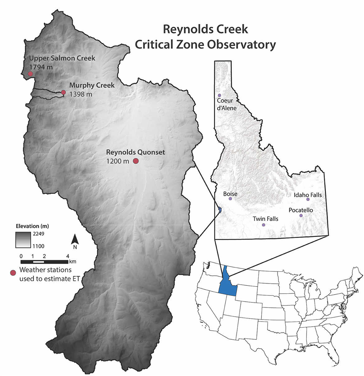
Figure 1. Map of the Reynolds Creek Critical Zone Observatory and Experimental Watershed with the three weather stations used to estimate ET. The Reynolds Quonset (43.205119°, −116.750273°) is the lowest elevation station, the Murphy Creek station (43.256298°, −116.8183291°) is the middle elevation member, and the highest station is the Upper Salmon Creek near Salmon Butte (43.266852°, −116.849919°).
Murphy Creek burned in 2015 during the Soda Fire (Vega et al., 2020), leaving riparian vegetation and hillslope grasses as the primary vegetation. The Murphy Creek riparian zone is densely vegetated with small bushes and willows that persist in a dry summer climate implying year-round subsurface flow. Hillslope and riparian vegetation can be clearly distinguished in person and in satellite images (Figure 2). Hillslopes are covered largely with mountain big sagebrush (Artemisia tridentata), bitterbrush (Purshia tridentata), Idaho fescue (Festuca idahoensis), Sandberg bluegrass (Poa secunda), bluebunch wheatgrass (Pseudoroegneria spicata), squirreltail grass (Elymus elymoides), and snowberry (Symphoricarpos spp.) (Pierson et al., 2000). In contrast, the channel is lined with riparian vegetation consisting of small bushes and willow, such as peach leaf willow (Salix amygdaloides), coyote willow (Salix exigua), red osier dogwood (Cornus sericea), woods rose (Rosa woodsii), chokecherry (Prunus virginiana), wax currant (Ribes cereum), and shrubby cinquefoil (Dasiphora fruticose) (personal communication with Mark Seyfried and Pat Clark).
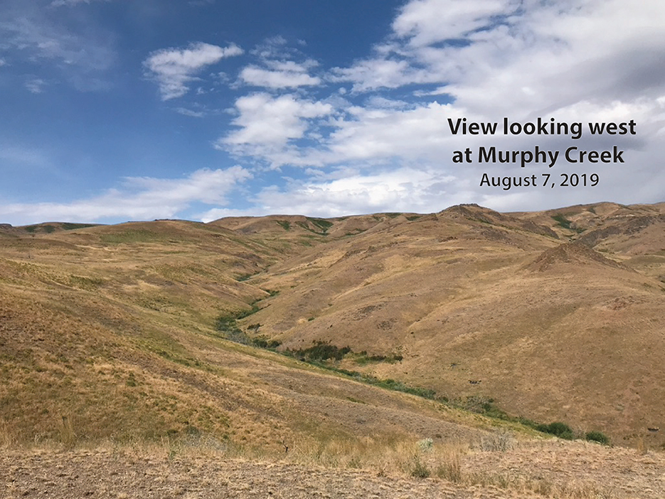
Figure 2. Photo of Murphy Creek looking west taken on August 7, 2019. Grasses and sagebrush on hillslopes are stark compared to the green riparian vegetation. This contrast enabled easy identification of the riparian zone in NDVI imagery. The willows and small bushes in the riparian zone require year-round water, while the surrounding hills covered with grasses and sagebrush have significantly lower water demands.
2.2. Flow presence and groundwater observations
Water presence or absence was observed with both freshwater HOBO electrical conductivity (EC) dataloggers (Onset HOBO logger, U-24) and HOBO Pendant Loggers (Onset HOBO Pendant/Light 64K Datalogger UA-002-64) that recorded relative electrical conductivity and temperature. The Pendant/Light 64K Dataloggers were modified following methods from Chapin et al. (2014). Twenty-one Pendant loggers were installed throughout Murphy Creek, and four EC loggers were interspersed between every five Pendant sensors (Figure 3). All loggers recorded at 15-min intervals from June 3, 2019 to October 1, 2019. Each Pendant sensor or EC logger is referred to as MX, where X is the distance in meters from the downstream outlet. A more detailed description of our field data collection process can be found in Warix et al. (2021) in Section 3.2.
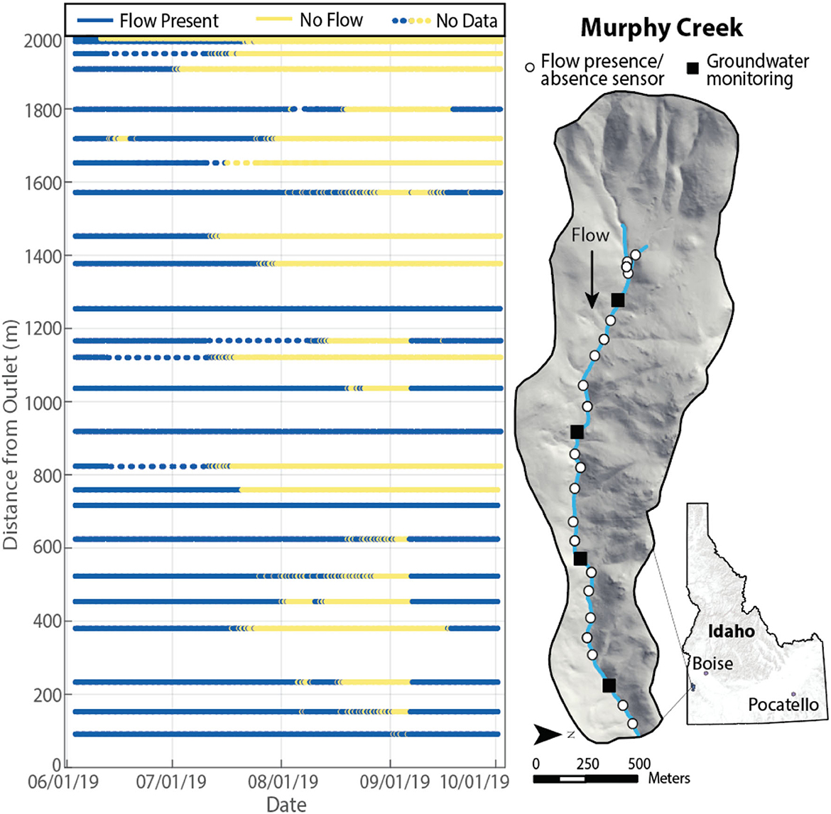
Figure 3. Hillshade map of Murphy Creek in the Reynolds Creek Experimental Watershed and Critical Zone Observatory. Each white circle (n = 21) indicates a Pendant flow presence sensor and each black square (n = 4) indicates a groundwater monitoring location, with both EC and WL loggers. In total, 25 sensors recorded water presence or absence from June 3, 2019 to October 1, 2019. Spatiotemporally distributed flow presence observations are displayed in the plot on the left-hand side. Each horizontal line represents a single sensor and is colored by the presence (blue) or absence (yellow) of surface flow. The lowermost line (91 meters upstream from the weir) represents the lowermost sensor. The uppermost line represents the highest elevation sensor in the watershed. All sensors were flowing at the beginning of the season. Twenty-two locations dried between June and early September, and of those, 11 rewetted before the end of the season. Diel cycling occurs where yellow and blue points alternate in quick succession.
We used all 25 sensors to analyze diel drying cycles, which were defined as any ~24-h cycling between the presence and absence of surface flow. Building from this, a “diel drying cycle period” was defined as a series of consecutive days with diel drying cycles, and this period can be interrupted by either complete rewetting or drying (a 24-h period with only wet or dry conditions). At each location that exhibited diel drying cycles, we extracted the time that drying began (drying start), the time that the stream rewetted (drying stop), and the total amount of time that the stream was dry (drying duration). For every diel cycle, we compared the time that the stream dried to the time that ET peaked. We extracted the drying duration from each day of each diel cycling period at the 25 flow presence monitoring locations. For each change in drying amplitude, we determined the change in total daily evapotranspiration. These metrics were selected so that we could compare changes in sub-daily drying patterns to variations in ET outputs.
2.3. Hierarchical clustering methods
To characterize patterns of drying, we used the entire season's flow presence data collected from all 25 sensors in Murphy Creek to create hierarchical clusters. Clusters were determined using Ward's method (Milligan, 1980) in JMP Pro 14; missing values were imputed by singular value decomposition.
2.4. Methods for determining groundwater inputs
Net lateral groundwater inputs to surface flow were calculated at four locations in Murphy Creek using a two-endmember mixing approach from Miller et al. (2014) detailed in Warix et al. (2021). Shallow piezometers were not installed due to permitting restrictions, and thus we determined net lateral groundwater inputs at 15-min timesteps at four locations from June 3 to October 1, 2019 using HOBO electrical conductivity (EC) dataloggers (Onset Hobologger, U-24) and water level (WL) dataloggers (Onset Hobologger, U-20) corrected with barometric pressure collected from a LI-7500RS Open Path CO2/H2O Analyzer at 30-min timesteps, and interpolated linearly to 15-min intervals to match the net lateral groundwater input measurements. We determined discharge from stage-discharge relationships based on periodic salt dilution gaging (Moore, 2003) paired with stage observations. More details on all methods are included in Warix et al. (2021) in Sections 3.2.1.1-3.
2.5. SMRF weather inputs
To model ET, local estimates of wind speed and direction, relative humidity, air temperature, and solar radiation were derived from three weather stations along an elevation gradient (1,200 m, 1,398 m, and 1,794 m) (Figure 1). All meteorological measurements were spatially interpolated to a 3-meter digital elevation model (DEM) using the Spatial Modeling for Resources Framework (SMRF, Havens et al., 2017). Using SMRF, air temperature and vapor pressure were interpolated with inverse distance weighting, accounting for elevational trends in the data. Wind speed and direction measurements were interpolated using topographic parameters that account for the local degree of exposure or sheltering (Winstral et al., 2002, 2009). Incoming solar radiation was also corrected for cloud cover, slope, aspect, and shading from the surrounding terrain (Dozier, 1980; Dozier and Frew, 1981; Dubayah, 1994).
2.6. Seasonal vegetation patterns: NDVI
Satellite imagery (3-m PSOrthoTiles) were acquired between June 2 and October 6, 2019 and were downloaded from Planet Lab (www.planet.com). Some satellite images were excluded from analysis, including those with cloud cover, skewed unrealistic images, and those with only partial watershed coverage. On average, one image was collected every 3 days; however, the largest time gap between retained images was 12 days. Images were collected each month of the study period, including June (10 images), July (8 images), August (13 images), September (10 images), and October (1 image). In total, NDVI was calculated for the entire watershed from 42 different images:
where NIR is the near-infrared band (Band 4, 780–860 nm) and Red is the red band (Band 3, 590–670 nm). An NDVI value for each 3 m × 3 m pixel containing each of the 25 flow sensors was extracted from each image and converted to a point value. Next, each NDVI point was grouped into one of four categories based on the flow status at the sensor: (1) flowing (continuous flow the day the image was collected and no previous drying), (2) diel drying cycle (between 0.25 and 23.75 h of drying the day the image was collected), (3) dry (continuously dry the day the image was collected), (4) rewetted (streamflow present for ≥24 h after drying at some point in the observation period). The range of dates that each flow group was observed (bounded by satellite image availability) were: flowing, June 2–October 6, 2019; diel, July 1–September 5, 2019; dry, June 12–October 6, 2019; and rewetted, September 13–October 6, 2019. There was overlap in the dates among the four groups because flow state varied among sensors (Figure 3). A one-way ANOVA test was run on each of the groups to test for significance. We recognize that NDVI varies seasonally, and thus temporal autocorrelation exists within the dataset, as discussed further in Section 4.2.
2.7. SHAW evapotranspiration calculations
We used the Simultaneous Heat and Water (SHAW) model to gain insight into groundwater dynamics, ET, and timing of streamflow drying. The SHAW model is a physically based simulation model that has been applied extensively over a range of vegetation types in semi-arid environments and shown to accurately simulate ET (e.g., Flerchinger et al., 1996, 2012, 2019; Chauvin et al., 2011; Flerchinger and Seyfried, 2014). It provides a numerical representation of a vertical, one-dimensional system composed of a multi-species plant canopy, snow cover (if present), plant residue, and the soil profile using the mixed form of the Richards equation (Figure 4; Celia et al., 1990). We used a version of the model that allowed for input of lateral subsurface flow into the soil profile, which was coupled to the Parameter Estimation & Uncertainty software, PEST (Doherty, 2005). For our application, input to the model included: hourly values of air temperature (T), wind speed (u), humidity (h), precipitation (i), and solar radiation (St); vegetation parameters; temporally varying leaf area index (LAI); and soil texture and hydraulic parameters. Net groundwater input observations were used as lateral input to the soil profile at the four sites with observations. At the 21 sites where groundwater input to streamflow was not collected, we simulated potential evapotranspiration (PET) using the SHAW model to compare timing and length of diel stream wetting/drying with ET; here we assume that PET closely approximates ET while the stream experiences diel wetting. Meteorological input for each site was based on spatially distributed estimates from the SMRF analysis (see Section 2.4).
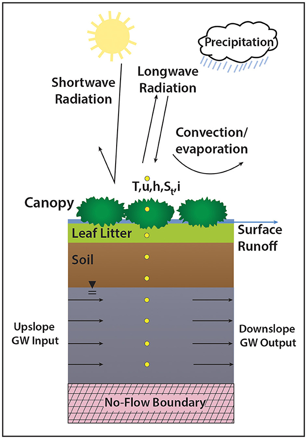
Figure 4. Conceptual diagram illustrating the SHAW model. Each yellow dot represents a model simulation node. See Section 2.7 for model details.
Vegetation characteristics (e.g., leaf area index and vegetation type, either tree, brush, or grass as determined by field observations and satellite imagery) input to the model were based on July 1 and September 1, 2019 NDVI values at each site (3 m Planet Images, see Section 2.6). Temporally varying LAI was estimated from NDVI values using the equation: LAI = 0.57*e2.33NDVI (Tewari et al., 2003), which yielded LAI values comparable to similar sites within the RC CZO (Flerchinger et al., 2016, 2019). Vegetation parameters were taken from previous SHAW simulations within the RC CZO according to observed vegetation type (i.e., trees, shrubs, or grasses). Soil depth and textural information were taken from similar sites in the watershed (Flerchinger et al., 2019; Patton et al., 2019).
Net lateral groundwater inputs to the model (upslope input minus downslope output; Figure 4) were based on measurements of total subsurface flow volume (L/s) for the stream corridor, described in Section 2.4. Groundwater measurements within the stream corridor were input to the model as uniform lateral input over the 2-m depth of the 1-m2 simulated profile (Figure 4). We assumed that groundwater was contributing over a 1-m2 area. However, there was uncertainty concerning the horizontal extent of groundwater flow, i.e., width of the stream corridor. Because data on stream corridor width over which sub-surface groundwater flow occurred were not available, it was necessary to optimize this value using the SHAW-PEST coupling.
The purpose of the PEST software is to minimize the weighted sum of squared differences between observed values and corresponding model outputs. In this case, the model output to be optimized was the presence or absence of runoff exiting the simulated soil profile, denoted with values of 1 and 0, respectively. Thus, time periods when the model incorrectly predicted the presence or absence of streamflow were minimized. In the absence of excess precipitation, runoff from the simulated profile was generated by seepage flow from the soil surface. Options in the SHAW-PEST coupling allow either: a PEST mathematical search for the optimized parameters through successive model runs; or a Monte Carlo analysis with model parameters randomly distributed within their specified ranges for each model run. In this case with only one parameter to optimize, the Monte Carlo analysis was chosen. Thirty-five simulations were run for each site with stream corridor widths randomly distributed between 5 and 40 m for each model run. Optimized stream corridor width for stations M233, M759, and M1799 were 5, 10, and 5 m, respectively. Because M1254 had continuous flow, it was not possible to optimize streamflow timing, and any width within the parameter range produced continuous flow, so a corridor width of 7.5 m (mid-way between that of M759 and M1799) was assumed.
Ideally, the optimized parameters would be validated with an independent data set, but given that only one year of data was available, this was not possible. Nevertheless, the detailed model simulations can provide insight into dynamics between groundwater, ET, and timing of stream drying.
3. Results
3.1. Spatiotemporal drying patterns and diel cycling
At the beginning of the observation period, flow was present at all 25 sensors (Figure 3). As the summer progressed, drying was heterogeneous in space and time throughout the stream; we observed three perennial locations and 22 non-perennial locations. Surface flow was interrupted by dry reaches at multiple points in the stream leading disconnected flowing reaches to appear throughout the network.
We observed that diel cycling and stream drying patterns did not occur linearly throughout the stream, but instead varied spatially (Figure 3). Hierarchical clustering shows that while stream headwaters were among the first to dry, distance downstream was not a primary control on the timing of stream drying. Together, Figures 3 and 5 show that stream locations hundreds of meters apart exhibited very similar stream drying behavior, despite being separated by locations with markedly different flowing or drying behavior.
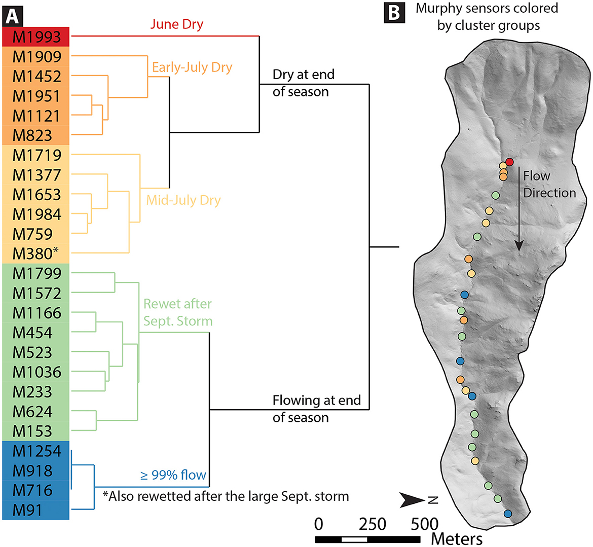
Figure 5. (A) Hierarchical cluster analysis results reveal five clusters colored by flow characteristics, including the timing and duration of drying patterns. From top to bottom in cluster order: the red group is M1984, the only sensor to dry in June; the orange group includes sensors that dried in early July and stayed dry through the season; the yellow group shows sensors that dried in mid-July and stayed dry through the season; the green group includes sensors that rewetted during an early September storm; and the blue group includes sensors that were flowing ≥99% of the season. (B) Map of Murphy Creek with the 25 sensors plotted on a hillshade. Sensors are colored by their cluster groups as displayed in (A).
We found that diel drying cycles (in which the stream cycled between wet and dry conditions with a 24-h period) often preceded persistent drying (>24 h of dry conditions). The start of drying was captured at 21 sensors, as indicated by the blue lines in June in Figure 3. Of those 21 sensors, 19 exhibited diel drying cycles prior to seasonal drying. Uninterrupted diel drying cycles lasted anywhere from two to 23 days and averaged 8 days. While diel drying periods often began at multiple sensors on the same day, these sensors were spatially disconnected by reaches that remained flowing (Figure 3). For example, M823, M1121, M1452, and M1951 all started diel cycles on June 10 despite persistent surface flow between each location. Eight locations started a period of diel cycling, then rewetted for a day or more before starting a second period of diel cycling.
The stream progressed through seasonal drying typical of the U.S. Intermountain West, and drying duration usually increased from day to day during diel drying periods (Figure 6). During diel drying periods, the time spent dry increased with each subsequent day (Figure 6) by an average of 1.16 ± 0.23 h/day (mean +/– s.d.). The onset of diel wet-dry periods typically occurred within 2 h of peak daily PET (Figure 7A) and diel drying duration tended to lengthen with increases in total daily PET (Figure 7B). However, we observed that the drying duration did not always increase linearly and that sometimes drying duration during a diel cycling period decreased for a single day before increasing again (Figure 7B). This is reflected in the relatively low R2 of the relationship between PET and drying duration, particularly when the absolute value of changes in daily PET were small.
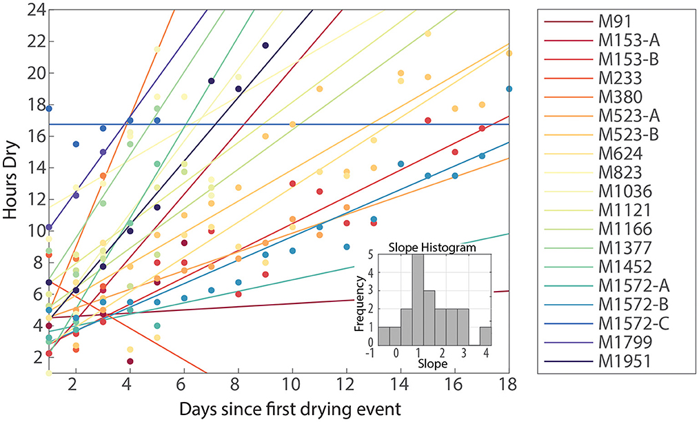
Figure 6. Diel cycling patterns were extracted from each of the sensors that exhibited diel drying. We plot the number of days that a single location has undergone continuous diel cycling against the duration of drying in hours during that day of the diel cycling period with the best-fit line for each set of data points plotted using the same color. If the stream was entirely dry or wet for at least 24 h, and later resumed a diel cycling of wetting and drying, a new data series was plotted for the same location, indicated by A-C adjacent to the site code in the legend. A histogram illustrating slope frequency of each best-fit line (n = 19) is plotted in the lower right-hand corner. All but two slopes are positive, and the median slope is 1.10 h/day, indicating that each additional day of drying led to a drying duration that was over an hour longer than the previous day.
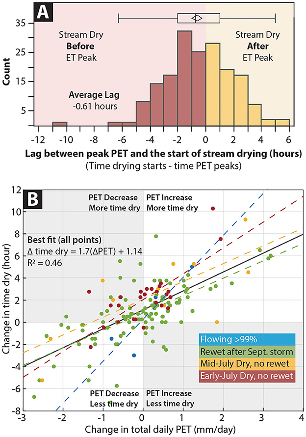
Figure 7. (A) Histogram of the difference between the time that drying started and the time that PET peaked during the same day of diel cycling at the 25 locations monitoring flow presence. The average lag was −0.16+/– 0.18 h, indicating the stream usually dried just before PET peaked. Over 95% of the time, the stream dried within ± 5 h of the time of peak ET. (B) Plot comparing the change in total daily PET against the change in time dry from one day to the next at a single location in a diel cycling period. Each point is colored by hierarchical clustering (detailed in Section 2.3 and Figure 5). Blue points were flowing for >99% of the season and green points rewetted after September storms. The yellow and red points dried in mid-July and early July, respectively, and did not rewet during the observation period. There is a positive relationship between the change in total daily ET and time spent dry, with an overall slope of 1.7 ± 0.16 hrdry/(mm/d) (mean slope +/– s.e.). However, for those locations that dried in early July and did not rewet (red points), the slopes were slightly higher [2.33 ± 0.42 hrdry/(mm/d)], thus indicating locations that might be more sensitive to a change in ET. Slopes were also higher for the handful of sites that remained flowing over 99% of the season, but the very low sample size (n = 4) and large uncertainty in the sensitivity [3.7 ± 1.3 hrdry/(mm/d)] suggest that any inferences for this group should be limited.
The relatively short lag between drying and peak daily PET (Figure 7A) suggests a responsive riparian aquifer and tight coupling between riparian ET and streamflow; such rapid connection has also been suggested in perennial diel cycling (Bond et al., 2002; Butler et al., 2007; Lautz, 2008; Gribovszki et al., 2010). In perennial systems, daily peaks and troughs in streamflow have been attributed to gains from snowmelt in systems with seasonal snowpacks during melt periods and to evapotranspiration outputs moderated by groundwater levels and the extent of riparian vegetation during groundwater-dominated periods (Bond et al., 2002; Gribovszki et al., 2010; Wondzell et al., 2010; Cadol et al., 2012; Kirchner et al., 2020). Further data collection that included in-stream and hyporheic water levels could facilitate more detailed analyses similar to those in perennial systems, but with both positive and negative (relative to stream bed) water levels.
3.2. Evapotranspiration, stream drying timing, and groundwater inputs
During the observation period, evapotranspiration typically peaked at 14:00 (MDT) each day at all 25 sites, and 60% of diel cycle drying started within ±2 h of peak ET (Figure 7A). Furthermore, when total daily ET increased from the previous day, the stream was more likely to spend a longer time dry; each 1 mm/day increase in total daily ET led to the stream drying 1.7 ± 0.14 h longer than the previous day (R2 = 0.46, p-value < 0.0001; Figure 7B). However, the moderate goodness-of-fit metric indicates additional possible controls on diel cycle periods.
At the four groundwater sites (Figure 1), we observed stream drying when evapotranspiration outputs exceeded groundwater inputs to surface flow (Figure 8) and focus on three instances near the onset of drying, as outlined in Figure 8A. The background of the plot denotes the presence (light blue) or absence (light yellow) of surface flow. Groundwater and ET from location M1799 are plotted for the week before and days after drying first started at this location (Figure 8B). Groundwater inputs are displayed as a dark blue shaded area and ET outputs (as modeled using SHAW) are displayed as green shaded area; groundwater is plotted on the right y-axis and ET is plotted on the left y-axis. As groundwater inputs decreased, evapotranspiration outputs stayed relatively constant. For example, when ET outputs exceeded groundwater inputs on 2 Aug, the stream dried. As ET dropped to zero that evening, surface flows resumed on 3 Aug, before seasonal drying commenced that afternoon. At all sites, the difference between evapotranspiration outputs and groundwater inputs decreased significantly over the season (black line in Figures 8C–E) and when this difference dropped below zero, the stream dried. At M1254, the stream never dried, and groundwater inputs were always higher than ET outputs (Figure 8D). However, the difference between groundwater and ET at this site was smallest when other locations were dry (mid-July to early September). Stream drying consistently occurred when evapotranspiration outputs exceeded groundwater inputs.
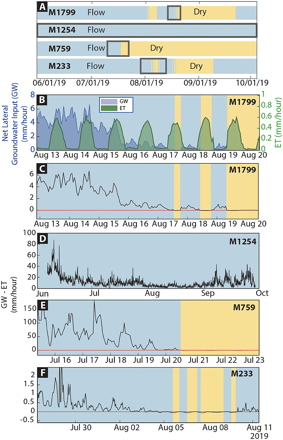
Figure 8. (A) Flow presence (blue) or absence (yellow) at each of the four groundwater monitoring stations throughout the experiment period with each subset outlined in black; similar background colors are used in all subsequent panels to indicate drying patterns. (B) Net lateral groundwater inputs (GW) and ET outputs from location M1799 are plotted for the 4 days before and 6 days after drying first started. The background of the plot denotes the presence (light blue) or absence (light yellow) of flow. GW inputs are displayed as a dark blue shaded area and ET outputs as modeled using SHAW are displayed green shaded area, GW is plotted on the right y-axis and ET is plotted on the left y-axis. Despite the different scales, the comparison is still valid because net groundwater inputs go to zero. When the green and blue polygons do not overlap (as in the right side of the plot), the stream is dry because ET outputs exceed net groundwater inputs. Different scales are required because of the large decrease in net groundwater inputs over the 10-day period. (C–F) The black line shows ET outputs (mm/hour) subtracted from GW inputs (mm/hour) and the red line shows 0. Negative values show when evapotranspiration outputs are greater than net groundwater inputs to surface flow, indicating when the stream dries.
3.3. Riparian NDVI and stream drying
Riparian NDVI values were significantly higher in areas with flowing water (seasonal average = 0.232 ± 0.045) and in diel cycling periods (seasonal average = 0.199 ± 0.043) than in areas that were dry (seasonal average = 0.168 ± 0.059) or areas that rewetted at the end of the season (seasonal average = 0.142 ± 0.035) (Figure 9). On average, after initial drying at a location, adjacent riparian NDVI dropped below 0.168 (median of all dry NDVI values) within 13 ± 2 days. Non-riparian hillslope vegetation primarily senesced in early July and we observed that these hillslopes always had considerably lower NDVI values than the riparian zone. Even though the riparian NDVI values are relatively low compared to global averages, they still reflect a locally green riparian zone (Figure 2). We also found a significant moderate correlation (R2 = 0.36, p = 3 × 10⁻⁵) between the average NDVI across all flow monitoring locations and the instantaneous flowing network extent (or percent of sensors exhibiting surface flow) at noon on the day the satellite image was collected (Figure 10).
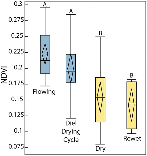
Figure 9. Box plots of NDVI categorized by flow condition. NDVI data was extracted at each of 25 sensors from 42 Planet images collected between June 2, 2019 and October 6, 2019. Flow categories are defined in section 2.6. NDVI was significantly greater at locations and times when the stream was flowing or in a diel cycling period (group A) as compared to drying and rewetting periods (group B).
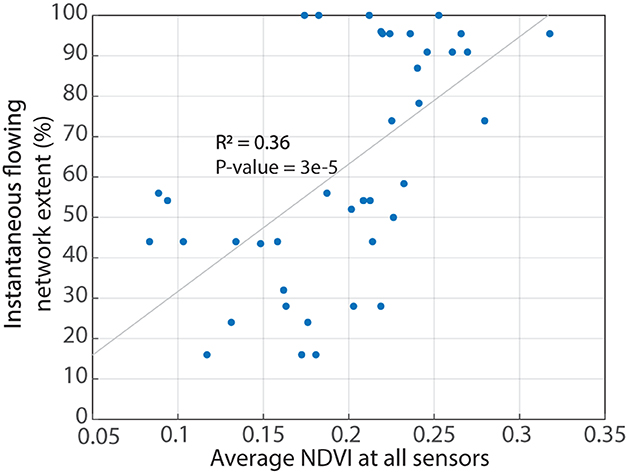
Figure 10. Average NDVI at all sensors is moderately correlated with the instantaneous flowing network extent (or the percent of sensors flowing at noon on the day the satellite image was collected).
4. Discussion
4.1. Diel cycling starts near peak ET when groundwater inputs are overcome
Because the delay between drying and peak ET is typically short (Figure 7A), this suggests that the riparian aquifer is very responsive (Kirchner et al., 2020). Our binary presence-absence data preclude the amplitude analysis common in perennial diel cycling studies, but analysis of the timing of drying still revealed differences among sites. The combination of seasonal increase in ET with daily increases in ET during the afternoon (due to diel cycles) was enough to reduce streamflow to zero during the diel drying period at most sites. Even though sites that are separated by 10s of meters have very similar climate and riparian vegetation, they exhibit different diel cycling patterns (Figures 3, 5). This implies that small changes in ET can be overridden by other factors, such as changes in topographic metrics that drive flow accumulation (see Prancevic and Kirchner, 2019; Warix et al., 2021), subsurface properties that affect the ability of groundwater to contribute to surface flow (Dohman et al., 2021; Warix et al., 2021), or variations in riparian vegetation density or distribution that lead to larger spatial variations in ET than initially expected.
Indeed, detailed SHAW modeling (Figures 8B–E) at the four groundwater sites revealed that stream drying begins when evapotranspiration outputs exceed groundwater inputs. Although spatial patterns of drying may be locally driven by tradeoffs between surface and subsurface flows (Godsey and Kirchner, 2014), our findings indicate that the timing of that drying also depends on local recharge and discharge to streams, and critically, on evapotranspiration. Controls on stream drying are not uniform throughout the length of a headwater stream and several local conditions must be satisfied for drying to occur. Drying only occurred at three of four groundwater monitoring locations despite all four having very similar seasonal ET outputs. We suggest that at location M1254 (where surface flow persisted throughout the season), and in other perennial segments of semi-arid streams headwater streams, a combination of physical attributes (i.e., favorable topographic and subsurface properties; Warix et al., 2021) enable surface flow to persist despite limited groundwater inputs. In contrast, the other three groundwater monitoring stations experienced drying because the correct geologic, geomorphic, and climatic attributes were met and the exact timing of drying occurred when (1) the location was no longer recharged either from precipitation and/or from deeper groundwater flow at a sufficient rate; and (2) local surface evapotranspiration outputs caused total discharge to decrease so that it could be entirely accommodated in the subsurface. The spatial and temporal scales of variability in evapotranspiration outputs are also important as local drying patterns may reflect heterogeneity over small scales over which evapotranspiration would typically be either temporally and or spatially averaged.
Together these observations suggest that spatiotemporal diel cycling patterns and the timing of seasonal drying are primed by the spatial drivers (e.g., geologic, geomorphic, and climatic factors, including those identified by Costigan et al., 2016 and Lovill et al., 2018). Once these spatial drivers are active and groundwater contributions have decreased, evapotranspiration outputs force stream drying to occur. This is supported by the observation that the difference between groundwater and evapotranspiration decreased until stream drying began (Figures 8B, C). During a diel cycling period, surface flow was present when groundwater inputs to the surface were greater than evaporation (Figure 11A), but the stream dried repeatedly when ET exceeded groundwater inputs (Figure 11B).
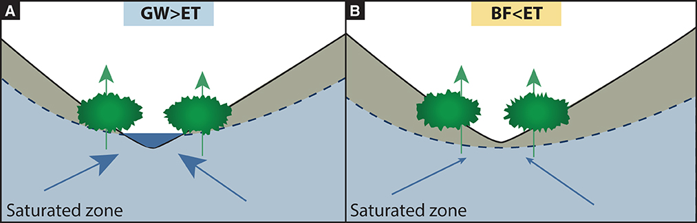
Figure 11. Conceptual diagram showing both groundwater inputs and ET outputs at the same location in two different scenarios. In both figures, the arrows are conceptual; flow may not be uniformly lateral and additional inputs may exist. When groundwater inputs exceed ET outputs, surface flow can persist (A) whereas if ET outputs are greater than groundwater inputs, and a dry channel occurs (B).
We were able to estimate variability in both ET and groundwater at spatial and temporal scales consistent with the observed drying patterns (sub-daily and at the scale of 10 s to 100 s of meters), which is important because local drying patterns may reflect heterogeneity at small scales over which evapotranspiration would typically be temporally and/or spatially averaged. This averaging can obscure differences in the timing of drying of local surface flow disconnections. Furthermore, groundwater and vegetation patterns may co-vary, leading to a negative feedback on local heterogeneity. To predict spatiotemporal drying variability and surface disconnections that may have a disproportionate ecological impact on aquatic species, we need to incorporate small temporal and spatial changes in stream drying controls.
4.2. Riparian NDVI weakly reflects stream drying patterns
These sub-daily, fine-scale patterns are also integrated into fine-scale variations in riparian vegetation characteristics. Riparian NDVI reflects the flow status (i.e., flowing, diel drying cycles, dry, rewet) of the stream during the groundwater recession period. By working with relatively fine spatial (3 m) and temporal (average time between images = 3 days) imagery, we found that riparian NDVI was higher when the stream was flowing or in a diel cycle period than when the stream was dry or after it had rewetted (Figure 9). Our findings are consistent with Fu and Burgher (2015) who observed riparian NDVI to correlate with shallow groundwater levels, decreasing during short periods of drying in Australian evergreen forests. However, riparian NDVI has not been widely used to predict flow status at fine temporal and spatial scales, and not in deciduous vegetation. It is possible that the spatiotemporal resolution of the images we analyzed allowed us to identify differences among groups that may have been previously undetectable; for reference, Landsat imagery such as those used by Fu and Burgher (2015) have 30-m pixels that were collected every 16 days. In addition, riparian NDVI in Murphy Creek was easy to identify because of the stark contrast between tan grassy hillslopes and green channels (Figure 2), so this method may be most effective where there are stark contrasts in vegetation between riparian areas and hillslopes.
The relationship between riparian NDVI and flow state is largely controlled by seasonal trends in NDVI. For example, early in the season in June when all monitored locations were flowing, the entire watershed was greener than in late August, and an analysis of seasonally detrended NDVI values shows no significant difference among the flow state groups. Furthermore, we expected NDVI responses to lag surface flow responses, as most vegetation relies on subsurface waters that may only indirectly reflect surface flow patterns (but see Newcomb and Godsey, 2023 for evidence of bidirectional linkages). Indeed, we observed that NDVI decreased most markedly at each site ~2 weeks after surface flows disappeared even though ET and NDVI remained uncorrelated over this time-period. Because of this lag, NDVI is not a good tool for predicting specific moments for stream drying and rewetting, but instead may improve predictions of watershed-wide seasonal patterns of drying. The moderate correlation between flow status and NDVI lacks the resolution to predict flow state at a given point (Figure 10). However, the good agreement between average riparian NDVI and the instantaneous flowing network extent highlights the potential for NDVI to inform larger scale surface flow models. Existing drying models (e.g., Ward et al., 2018; Jaeger et al., 2019) require extensive parameterization and/or field observations, neither of which is required by NDVI. We suggest that the relationship between high-resolution NDVI and flow status be further explored as the potential for predicting point-scale stream drying patterns from remotely sensed images is high. This potential must still be assessed with additional ground-truthing.
5. Conclusions
We present three primary conclusions based on observations from a semi-arid, groundwater-supported, headwater stream: (1) during a diel cycling period, stream drying is most likely to start within 2 h of peak evapotranspiration (Figure 7A), (2) surface drying occurs when evapotranspiration outputs exceed groundwater inputs to the surface (Figure 8), and (3) a weak relationship exists between riparian NDVI and flow status (Figure 9). Most notably, the tight coupling between evapotranspiration outputs, groundwater inputs, and the timing of drying suggests the following framework for understanding heterogeneity in the timing of drying. Surface drying occurs at a given location when (1) the correct geologic, geomorphic, and climatic attributes are met (Warix et al., 2021); (2) the location is no longer recharged either from precipitation and/or from deeper groundwater flow at a sufficient rate; and (3) local outputs cause total discharge to decrease so that it can be entirely accommodated in the subsurface (Figure 11). Any heterogeneity in these three metrics may cause neighboring locations to vary significantly in their stream drying patterns. Finally, we suggest the relationship between riparian NDVI and surface flow status be further explored because of the potential for a low-cost remotely-sensed stream drying model. We expect that these conclusions also drive the timing of drying in other semi-arid, groundwater-supported, headwater streams, but note that fine-scale ET and drying data remain scarce, and thus transferrable conclusions will be strengthened by increased ET and drying observations in other catchments.
Data availability statement
The datasets presented in this study can be found in online repositories. The names of the repository/repositories and accession number(s) can be found below: doi: 10.18122/reynoldscreek/22/boisestate.
Author contributions
SW: Conceptualization, Data curation, Formal analysis, Investigation, Methodology, Visualization, Writing—original draft, Writing—review and editing. SG: Funding acquisition, Investigation, Methodology, Project administration, Resources, Writing—review and editing. GF: Data curation, Formal analysis, Investigation, Methodology, Writing—original draft, Writing—review and editing. SH: Data curation, Investigation, Methodology, Writing—review and editing. KL: Funding acquisition, Project administration, Resources, Supervision, Writing—review and editing. HB: Supervision, Writing—review and editing. XC: Formal analysis, Methodology, Writing—review and editing. RH: Methodology, Writing—review and editing. MS: Writing—review and editing.
Funding
The author(s) declare financial support was received for the research, authorship, and/or publication of this article from NSF EAR 1653998 & RC CZO Coop Agreement EAR 1331872, Exxon Mobil, the Idaho State University Geslin Fund, and the Geological Society of America.
Acknowledgments
This research was performed in collaboration with the USDA Agricultural Research Service, Northwest Watershed Research Center in Boise, Idaho, and the landowners within the Reynolds Creek Experimental Watershed and Critical Zone Observatory. We would like to thank the USDA-Agricultural Research Service, particularly Zane Cram and Barry Caldwell. The Reynolds Creek Experimental Watershed is administered by the USDA ARS and supported by the USDA Long-Term Agroecosystem Research (LTAR) network. In addition, we would like to thank NSF EAR 1653998 & RC CZO Coop Agreement EAR 1331872, Exxon Mobil, the Idaho State University Geslin Fund, and the Geological Society of America for project funding. We thank Planet.com for providing satellite imagery for academic use. Finally, we would like to thank Inbar Milstein and Logan Mahoney for field assistance.
Conflict of interest
The authors declare that the research was conducted in the absence of any commercial or financial relationships that could be construed as a potential conflict of interest.
Publisher's note
All claims expressed in this article are solely those of the authors and do not necessarily represent those of their affiliated organizations, or those of the publisher, the editors and the reviewers. Any product that may be evaluated in this article, or claim that may be made by its manufacturer, is not guaranteed or endorsed by the publisher.
References
Aguilar, C., Zinnert, J. C., Polo, M. J., and Young, D. R. (2012). NDVI as an indicator for changes in water availability to woody vegetation. Ecol. Indic. 23, 290–300. doi: 10.1016/j.ecolind.2012.04.008
Bond, B. J., Jones, J. A., Moore, G., Phillips, N., Post, D., and McDonnell, J. J. (2002). The zone of vegetation influence on baseflow revealed by diel patterns of streamflow and vegetation water use in a headwater basin. Hydrol. Proc. 16, 1671–1677. doi: 10.1002/hyp.5022
Boronina, A., Golubev, S., and Balderer, W. (2005). Estimation of actual evapotranspiration from an alluvial aquifer of the Kouris catchment (Cyprus) using continuous streamflow records. Hydrol. Proc. 19, 4055–4068. doi: 10.1002/hyp.5871
Botter, G., and Durighetto, N. (2020). The stream length duration curve: a tool for characterizing the time variability of the flowing stream length. Water Resour. Res. 56, e2020WR027282. doi: 10.1029/2020WR027282
Butler, J. J., Kluitenberg, G. J., Whittemore, D. O., Loheide, S. P., Jin, W., Billinger, M. A., et al. (2007). A field investigation of phreatophyte-induced fluctuations in the water table. Water Resour. Res. 43, 1–12. doi: 10.1029/2005WR004627
Cadol, D., Kampf, S., and Wohl, E. (2012). Effects of evapotranspiration on baseflow in a tropical headwater catchment. J. Hydrol. 462, 4–14. doi: 10.1016/j.jhydrol.2012.04.060
Celia, M. A., Bouloutas, E. T., and Zarba, R. L. (1990). A general mass-conservative numerical solution for the unsaturated flow equation. Water Resour. Res. 26, 1483–1496. doi: 10.1029/WR026i007p01483
Chapin, T. P., Todd, A. S., and Zeigler, M. P. (2014). Robust, low-cost data loggers for stream temperature, flow intermittency, and relative conductivity monitoring. Water Resour. Res. 50, 6542–6548.
Chauvin, G. M., Flerchinger, G. N., Link, T. E., Marks, D., Winstral, A. H., and Seyfried, M. S. (2011). Long-term water balance and conceptual model of a semi-arid mountainous catchment. J. Hydrol. 400, 133–143. doi: 10.1016/j.jhydrol.2011.01.031
Costigan, K. H., Jaeger, K. L., Goss, C. W., Fritz, K. M., and Goebel, P. C. (2016). Understanding controls on flow permanence in intermittent rivers to aid ecological research: integrating meteorology, geology and land cover. Ecohydrology 9, 1141–1153. doi: 10.1002/eco.1712
Daiji, K., Suzuki, K., and Nomura, M. (1990). Diurnal fluctuation in stream flow and in specific electric conductance during drought periods. J. Hydrol. 115, 105–114. doi: 10.1016/0022-1694(90)90200-H
Datry, T., Larned, S. T., and Tockner, K. (2014). Intermittent rivers: a challenge for freshwater ecology. BioScience 64, 229–235. doi: 10.1093/biosci/bit027
Doherty, J. (2005). PEST: Model-Independent Parameter Estimation User Manual. 5th Edition. Available online at: http://www.pesthomepage.org/ (accessed June 1, 2023).
Dohman, J. M., Godsey, S. E., and Hale, R. L. (2021). Three-dimensional subsurface flow path controls on flow permanence. Water Resour. Res. 57, 1–18. doi: 10.1029/2020WR028270
Dozier, J. (1980). A clear-sky spectral solar radiation model for snow-covered mountainous terrain. Water Resour. Res. 16, 709–718. doi: 10.1029/WR016i004p00709
Dozier, J., and Frew, J. (1981). Atmospheric corrections to satellite radiometric data over rugged terrain. Rem. Sens. Environ. 11, 191–205. doi: 10.1016/0034-4257(81)90019-5
Dubayah, R. C. (1994). Modeling a solar radiation topoclimatology for the Rio Grande River Basin. J. Veget. Sci. 5, 627–640. doi: 10.2307/3235879
Eng, K., Wolock, D. M., and Dettinger, M. D. (2015). Sensitivity of intermittent streams to climate variations in the USA. River Res. Applic. 32, 885–895. doi: 10.1002/rra.2939
Fahle, M., and Dietrich, O. (2014). Estimation of evapotranspiration using diurnal groundwater level fluctuations: Comparison of different approaches with groundwater lysimeter data. Water Resour. Res. 50, 273–286. doi: 10.1002/2013WR014472
Flerchinger, G.erald N., Fellows, A. W., Seyfried, M. S., Clark, P. E., and Lohse, K. A. (2019). Water and carbon fluxes along an elevational gradient in a sagebrush ecosystem. Ecosystems 23, 246–263. doi: 10.1007/s10021-019-00400-x
Flerchinger, G.erald N., Reba, M. L., and Marks, D. (2012). Measurement of surface energy fluxes from two rangeland sites and comparison with a multilayer canopy model. J. Hydrometeorol. 13, 1038–1051. doi: 10.1175/JHM-D-11-093.1
Flerchinger, G. N., Hanson, C. L., and Wight, J. R. (1996). Modeling evapotranspiration and surface energy budgets across a watershed. Water Resour. Res. 32, 2539–2548. doi: 10.1029/96WR01240
Flerchinger, G. N., and Seyfried, M. S. (2014). Comparison of methods for estimating evapotranspiration in a small rangeland catchment. Vadose Zone J. 13, vzj2013.08.0152. doi: 10.2136/vzj2013.08.0152
Flerchinger, G. N., Seyfried, M. S., and Hardegree, S. P. (2016). Hydrologic response and recovery to prescribed fire and vegetation removal in a small rangeland catchment. Ecohydrology 9, 1604–1619. doi: 10.1002/eco.1751
Fritz, K. M., Schofield, K. A., Alexander, L. C., McManus, M. G., Golden, H. E., Lane, C. R., et al. (2018). Physical and chemical connectivity of streams and riparian wetlands to downstream waters: a synthesis. J. Am. Water Resour. Assoc. 54, 323–345. doi: 10.1111/1752-1688.12632
Fu, B., and Burgher, I. (2015). Riparian vegetation NDVI dynamics and its relationship with climate, surface water and groundwater. J. Arid Environ. 113, 59–68. doi: 10.1016/j.jaridenv.2014.09.010
Geisler, E. T. (2016). Riparian zone evapotranspiration using streamflow diel signals. Boise State University Theses and Dissertations.
Godsey, S. E., and Kirchner, J. W. (2014). Dynamic, discontinuous stream networks: Hydrologically driven variations in active drainage density, flowing channels and stream order. Hydrol. Proc. 28, 5791–5803. doi: 10.1002/hyp.10310
González-Ferreras, A. M., and Barquín, J. (2017). Mapping the temporary and perennial character of whole river networks. Water Resour. Res. 53, 6709–6724. doi: 10.1002/2017WR020390
Gribovszki, Z., Szilágyi, J., and Kalicz, P. (2010). Diurnal fluctuations in shallow groundwater levels and streamflow rates and their interpretation: a review. J. Hydrol. 385, 371–383. doi: 10.1016/j.jhydrol.2010.02.001
Hale, R. L., and Godsey, S. E. (2019). Dynamic stream network intermittence explains emergent dissolved organic carbon chemostasis in headwaters. Hydrol. Proc. 33, 1926–1936. doi: 10.1002/hyp.13455
Hammond, J. C., Zimmer, M., Shanafield, M., Kaiser, K., Godsey, S. E., Mims, M. C., et al. (2021). Spatial patterns and drivers of nonperennial flow regimes in the contiguous United States. Geophy. Res. Lett. 48, 1–11. doi: 10.1029/2020GL090794
Harmon, R., Barnard, H. R., and Singha, K. (2020). Water table depth and bedrock permeability control magnitude and timing of transpiration-induced diel fluctuations in groundwater. Water Resour. Res. 56, 1–22. doi: 10.1029/2019WR025967
Havens, S., Marks, D., Kormos, P., and Hedrick, A. (2017). Spatial modeling for resources framework (SMRF): A modular framework for developing spatial forcing data for snow modeling in mountain basins. Comput. Geosci. 109, 295–304. doi: 10.1016/j.cageo.2017.08.016
Heilweil, B. V. M., Solomon, D. K., and Gardner, P. M. (2002). Infiltration and Recharge at Sand Hollow, an Upland Bedrock Basin in Southwestern Utah. US Geological Survey.
Hoffmann, J. P., Blasch, K. W., Pool, D. R., Bailey, M. A., and Callegary, J. B. (2007). “Estimated infiltration, percolation, and recharge rates at the Rillito Creek focused recharge investigation site, Pima County, Arizona: USGS Professional Paper 1703-H,” in Ground-Water Recharge in the Arid and Semiarid Southwestern United States: USGS Professional Paper 1703-H, 187–220. Available online at: https://pubs.usgs.gov/pp/pp1703/h/ (accessed June 1, 2023).
Izbicki, J. A., Johnson, R. U., Kulongoski, J., and Predmore, S. (2007). Ground-water recharge from small intermittent streams in the western Mojave desert, California. Ground-Water Recharge in the Arid and Semiarid Southwestern United States, Chapter G. doi: 10.3133/pp1703G
Jaeger, K. L., Sando, R., McShane, R. R., Dunham, J. B., Hockman-Wert, D. P., Kaiser, K. E., et al. (2019). Probability of streamflow permanence model (PROSPER): A spatially continuous model of annual streamflow permanence throughout the Pacific Northwest. J. Hydrol. X 2, 100005. doi: 10.1016/j.hydroa.2018.100005
Jensen, C. K., McGuire, K. J., McLaughlin, D. L., and Scott, D. T. (2019). Quantifying spatiotemporal variation in headwater stream length using flow intermittency sensors. Environ. Monitor. Assess. 191, 226. doi: 10.1007/s10661-019-7373-8
Jensen, C. K., McGuire, K. J., Shao, Y., and Andrew Dolloff, C. (2018). Modeling wet headwater stream networks across multiple flow conditions in the Appalachian Highlands. Earth Surf. Proc. Landforms 43, 2762–2778. doi: 10.1002/esp.4431
Kirchner, J., Godsey, S., Osterhuber, R., McConnell, J., and Penna, D. (2020). “The pulse of a montane ecosystem: coupled daily cycles in solar flux, snowmelt, transpiration, groundwater, and streamflow at Sagehen and Independence Creeks, Sierra Nevada, USA,” in Hydrology and Earth System Sciences Discussions 1–46. doi: 10.5194/hess-2020-77
Klausmeyer, K., Howard, J., Keeler-wolf, T., Davis-fadtke, K., and Hull, R. (2018). Mapping indicators of groundwater dependent ecosystems in California: Methods report. San Francisco, California.
Kormos, P. R., Marks, D., Seyfried, M., Havens, S., Hendrick, A., Lohse, K. A., et al. (2016). 31 years of spatially distributed air temperature, humidity, precipitation amount and precipitation phase from a mountain catchment in the rain-snow transition zone. Data set.
Lautz, L. K. (2008). Estimating groundwater evapotranspiration rates using diurnal water-table fluctuations in a semi-arid riparian zone. Hydrogeol. J. 16, 483–497. doi: 10.1007/s10040-007-0239-0
Lovill, S. M., Hahm, W. J., and Dietrich, W. E. (2018). Drainage from the critical zone: lithologic controls on the persistence and spatial extent of wetted channels during the summer dry season. Water Resour. Res. 54, 5702–5726. doi: 10.1029/2017WR021903
MacNeille, R. B., Lohse, K. A., Godsey, S. E., and Perdrial, J. N. (2020). Influence of drying and wildfire on longitudinal chemistry patterns and processes of intermittent streams. Front. Water 2, 563841. doi: 10.3389/frwa.2020.563841
McIntyre, D. H. (1972). Cenozoic geology of the Reynolds Creek Experimental Watershed, Owyhee County, Idaho. Idaho Bureau Mines Geolo. Pamphlet P-151.
Miller, M. P., Susong, D. D., Shope, C. L., Heilweil, V. M., and Stolp, B. J. (2014). Continuous estimation of baseflow in snowmelt-dominated streams and rivers in the Upper Colorado River Basin: a chemical hydrograph separation approach. Water Resour. Res. 50, 6986–6999. doi: 10.1002/2013WR014939
Milligan, G. W. (1980). An examination of the effect of six types of error perturbation on fifteen clustering algorithms. Psychometrika 45, 325–342. doi: 10.1007/BF02293907
Moidu, H., Obedzinski, M., Carlson, S. M., and Grantham, T. E. (2021). Spatial patterns and sensitivity of intermittent stream drying to climate variability. Water Resour. Res. 57, 1–14. doi: 10.1029/2021WR030314
Moore, R. D. D. (2003). Introduction to salt dilution gauging for streamflow measurement: part streamline. Watershed Manage. Bull. 7, 20–23.
Nadeau, T. L., and Rains, M. C. (2007). Hydrological connectivity between headwater streams and downstream waters: How science can inform policy. J. Am. Water Resour. Assoc. 43, 118–133. doi: 10.1111/j.1752-1688.2007.00010.x
Nagler, P. L., Jarchow, C. J., and Glenn, E. P. (2018). Remote sensing vegetation index methods to evaluate changes in greenness and evapotranspiration in riparian vegetation in response to the Minute 319 environmental pulse flow to Mexico. Proc. Int. Assoc. Hydrol. Sci. 380, 45–54. doi: 10.5194/piahs-380-45-2018
Newcomb, S. K., and Godsey, S. E. (2023). Nonlinear riparian interactions drive changes in headwater streamflow. Water Resour. Res. 2023, 1–18. doi: 10.1029/2023WR034870
Patton, N. R., Lohse, K. A., Seyfried, M., Will, R., and Benner, S. G. (2019). Lithology and coarse fraction adjusted bulk density estimates for determining total organic carbon stocks in dryland soils. Geoderma 337, 844–852. doi: 10.1016/j.geoderma.2018.10.036
Pierson, F. B., Slaughter, C. W., and Cram, Z. K. (2000). Monitoring discharge and suspended sediment, Reynolds Creek Experimental Watershed, Idaho, USA. ARS Technical Bulletin NWRC. doi: 10.1029/2001WR000420
Prancevic, J. P., and Kirchner, J. W. (2019). Topographic controls on the extension and retraction of flowing streams. Geophy. Res. Lett. 46, 2084–2092. doi: 10.1029/2018GL081799
Queener, N. (2015). Spatial and temporal variability in baseflow and stream drying in the Mattole River Headwaters. Technical report, Humboldt State University. doi: 10.5194/hess-2016-300
Rau, G. C., Halloran, L. J. S., Cuthbert, M. O., Andersen, M. S., Acworth, R. I., and Tellam, J. H. (2017). Characterising the dynamics of surface water-groundwater interactions in intermittent and ephemeral streams using streambed thermal signatures. Adv. Water Resour. 107, 354–369. doi: 10.1016/j.advwatres.2017.07.005
Reynolds, L. V., Shafroth, P. B., and LeRoy Poff, N. (2015). Modeled intermittency risk for small streams in the Upper Colorado River Basin under climate change. J. Hydrol. 523, 768–780. doi: 10.1016/j.jhydrol.2015.02.025
Runkel, R. L., McKnight, D. M., and Andrews, E. D. (2016). Analysis of transient storage subject to unsteady flow : diel flow variation in an antarctic stream. J. North Am. Benthol. Soc. 17, 143–154. doi: 10.2307/1467958
Shanafield, M., Gutiérrez-Jurado, H., Rodríguez-Burgueño, J. E., Ramírez-Hernández, J., Jarchow, C. J., and Nagler, P. L. (2017). Short- and long-term evapotranspiration rates at ecological restoration sites along a large river receiving rare flow events. Hydrol. Proc. 31, 4328–4337. doi: 10.1002/hyp.11359
Stewart-Deaker, A. E., Stonestrom, D. A., and Moore, S. J. (2000). Streamflow, infiltration, and ground-water recharge at Abo Arroyo, New Mexico. US Geological Survey Professional Paper, 83–106. doi: 10.3133/pp1703D
Sullivan, A. B., and Drever, J. I. (2001). Spatiotemporal variability in stream chemistry in a high-elevation catchment affected by mine drainage. J. Hydrol. 252, 237–250. doi: 10.1016/S0022-1694(01)00458-9
Tewari, S., Kulhavý, J., Rock, B. N., and Hadaš, P. (2003). Remote monitoring of forest response to changed soil moisture regime due to river regulation. J. Forest Sci. 49, 429–438. doi: 10.17221/4716-JFS
US EPA (2015). US and Environmental Protection Agency, and U S, Army Corps of Engineers. Technical Support Document for the Clean Water Rule: Definition of Waters of the United States. U.S. Environmental Protection Agency.
Vega, S. P., Williams, C. J., Brooks, E. S., Pierson, F. B., Strand, E. K., Robichaud, P. R., et al. (2020). Interaction of wind and cold-season hydrologic processes on erosion from complex topography following wildfire in sagebrush steppe. Earth Surf. Proc. Landforms 45, 841–861. doi: 10.1002/esp.4778
Villeneuve, S., Cook, P. G., Shanafield, M., Wood, C., and White, N. (2015). Groundwater recharge via infiltration through an ephemeral riverbed, central Australia. J. Arid Environ. 117, 47–58. doi: 10.1016/j.jaridenv.2015.02.009
Ward, A. S., Schmadel, N. M., and Wondzell, S. M. (2018). Simulation of dynamic expansion, contraction, and connectivity in a mountain stream network. Adv. Water Resour. 114, 64–82. doi: 10.1016/j.advwatres.2018.01.018
Warix, S. R., Godsey, S. E., Lohse, K. A., and Hale, R. L. (2021). Influence of groundwater and topography on stream drying in semi-arid headwater streams. Hydrol. Proc. 35, 1–18. doi: 10.1002/hyp.14185
Werstak, C. E. J., Housman, I., Maus, P., Fisk, H., Gurrieri, J., Carlson, C. P., et al. (2010). Groundwater-Dependent Ecosystem Inventory Using Remote Sensing. RSAC-10011-RPT1, U.S. Department of Agriculture, Forest Service, Remote Sensing Applications Center. Available online at: https://www.fs.usda.gov/Internet/FSE_DOCUMENTS/stelprdb5405946.pdf (accessed June 1, 2023).
White, W. N. (1932). A method of estimating ground-water supplies based on discharge by plants and evaporation from soil. USGS Water-Supply Paper No. 659–A.
Winstral, A., Elder, K., and Davis, R. E. (2002). Spatial snow modeling of wind-redistributed snow using terrain-based parameters. J. Hydrometeorol. 3, 524–538. doi: 10.1175/1525-7541(2002)003<0524:SSMOWR>2.0.CO;2
Winstral, A., Marks, D., and Gurney, R. (2009). An efficient method for distributing wind speeds over heterogeneous terrain. Hydrol. Proc. 23, 2526–2535. doi: 10.1002/hyp.7141
Wondzell, S. M., Gooseff, M. N., and McGlynn, B. L. (2010). An analysis of alternative conceptual models relating hyporheic exchange flow to diel fluctuations in discharge during baseflow recession. Hydrol. Proc. 24, 686–694. doi: 10.1002/hyp.7507
Yu, S., Bond, N. R., Bunn, S. E., Xu, Z., and Kennard, M. J. (2018). Quantifying spatial and temporal patterns of flow intermittency using spatially contiguous runoff data. J. Hydrol. 559, 861–872. doi: 10.1016/j.jhydrol.2018.03.009
Keywords: evapotranspiration, groundwater/surface water interaction, remote sensing, streamflow, intermittent streams
Citation: Warix SR, Godsey SE, Flerchinger G, Havens S, Lohse KA, Bottenberg HC, Chu X, Hale RL and Seyfried M (2023) Evapotranspiration and groundwater inputs control the timing of diel cycling of stream drying during low-flow periods. Front. Water 5:1279838. doi: 10.3389/frwa.2023.1279838
Received: 18 August 2023; Accepted: 03 October 2023;
Published: 25 October 2023.
Edited by:
Dipankar Dwivedi, Berkeley Lab (DOE), United StatesReviewed by:
Masato Kobiyama, Federal University of Rio Grande do Sul, BrazilDavid E. Rheinheimer, California Natural Resources Agency, United States
Copyright © 2023 Warix, Godsey, Flerchinger, Havens, Lohse, Bottenberg, Chu, Hale and Seyfried. This is an open-access article distributed under the terms of the Creative Commons Attribution License (CC BY). The use, distribution or reproduction in other forums is permitted, provided the original author(s) and the copyright owner(s) are credited and that the original publication in this journal is cited, in accordance with accepted academic practice. No use, distribution or reproduction is permitted which does not comply with these terms.
*Correspondence: Sara R. Warix, c3dhcml4QG1pbmVzLmVkdQ==
†Present address: Rebecca L. Hale, Smithsonian Environmental Research Center, Edgewater, MD, United States