 Mohammad Zeynoddin
 Silvio José Gumiere
 Hossein Bonakdari2
94% of researchers rate our articles as excellent or good
Learn more about the work of our research integrity team to safeguard the quality of each article we publish.
Find out more
ORIGINAL RESEARCH article
Front. Water, 22 August 2023
Sec. Water and Hydrocomplexity
Volume 5 - 2023 | https://doi.org/10.3389/frwa.2023.1237592
This article is part of the Research TopicHydro-informatics for Sustainable Water Management in Agrosystems - Volume IIView all 6 articles
Real-time soil matric potential measurements for determining potato production's water availability are currently used in precision irrigation. It is well known that managing irrigation based on soil matric potential (SMP) helps increase water use efficiency and reduce crop environmental impact. Yet, SMP monitoring presents challenges and sometimes leads to gaps in the collected data. This research sought to address these data gaps in the SMP time series. Using meteorological and field measurements, we developed a filtering and imputation algorithm by implementing three prominent predictive models in the algorithm to estimate missing values. Over 2 months, we gathered hourly SMP values from a field north of the Péribonka River in Lac-Saint-Jean, Québec, Canada. Our study evaluated various data input combinations, including only meteorological data, SMP measurements, or a mix of both. The Extreme Learning Machine (ELM) model proved the most effective among the tested models. It outperformed the k-Nearest Neighbors (kNN) model and the Evolutionary Optimized Inverse Distance Method (gaIDW). The ELM model, with five inputs comprising SMP measurements, achieved a correlation coefficient of 0.992, a root-mean-square error of 0.164 cm, a mean absolute error of 0.122 cm, and a Nash-Sutcliffe efficiency of 0.983. The ELM model requires at least five inputs to achieve the best results in the study context. These can be meteorological inputs like relative humidity, dew temperature, land inputs, or a combination of both. The results were within 5% of the best-performing input combination we identified earlier. To mitigate the computational demands of these models, a quicker baseline model can be used for initial input filtering. With this method, we expect the output from simpler models such as gaIDW and kNN to vary by no more than 20%. Nevertheless, this discrepancy can be efficiently managed by leveraging more sophisticated models.
Water scarcity continues to be a significant barrier to agricultural productivity. Enhancing the efficiency of water use in agriculture is a crucial challenge to achieve higher crop yields (Molden et al., 2010; Chen et al., 2018; Matteau et al., 2021). Despite agriculture being the primary consumer of the Earth's freshwater, competition from other sectors is intensifying. Governments frequently advocate for improved irrigation efficiency to balance this demand (FAO, 2008).
Real-time Soil Matric Potential (SMP) measurements are essential in this context. Irrigation management strategies based on SMP can enhance water productivity and increase yield (Matteau et al., 2021, 2022b). However, crops' optimal irrigation thresholds based on SMP vary (Rekika et al., 2014; Létourneau et al., 2015; Périard et al., 2015). Consequently, personalized irrigation strategies based on crop-specific SMP ranges can help prevent over-irrigation or water deficiency (Matteau et al., 2022a). Yet, SMP real-time measurements can generate unstructured and messy data impairing decision-making and predictive modeling performance (Kamilaris and Prenafeta-Boldú, 2018). These unstructured and missing data (UMD) impede the effective implementation of data-driven methods, like precision agriculture and machine learning, leading to less-than-optimal farming strategies and inefficient resource utilization. This issue is especially pressing given the need for sustainable farming practices to meet increasing global food demand while minimizing environmental impacts (Godfray et al., 2010).
UMD, often a result of equipment failure, data entry errors, or data loss, is another pressing issue, particularly given that measurements are taken under conditions heavily influenced by natural environmental circumstances (Di Piazza, 2011; Fountas et al., 2015; Wolfert et al., 2017; Bleidorn et al., 2022). Dealing with missing data effectively reduces estimation bias and improves parameter accuracy (Rouzinov and Berchtold, 2022).
Several strategies exist to address UMD. The primary strategy is deletion when data are missing at random and unrelated to the variable itself (Allison, 2003) or the missing rate is < 5% (Dong and Peng, 2013). However, when the missing rate surpasses 10%, biased results are likely (Bennett, 2001). In such situations, statistical and artificial estimation methods prove useful. For instance, in environmental research, it is often assumed that neighboring sites can significantly contribute to data reconstruction (Cheng and Lu, 2017). Therefore, spatial and temporal interpolation methods are commonly used (Tonini et al., 2016; Tipton et al., 2017).
Notably, Inverse Distance Weighting (IDW), kriging, and cokriging methods, along with their variants, are widely adopted for this purpose (Eskelson et al., 2009; Bhattacharjee et al., 2014). Among them, IDW methods like harmony search-IDW, genetic algorithm (ga)-IDW, and particle swarm-IDW are the most reliable for estimating missing environmental data (Chang et al., 2005; Gholipour et al., 2013; Li and Wang, 2013; Barbulescu et al., 2020). E.g., Bárbulescu et al. (2021) affirmed the reliability of gaIDW, demonstrating that its accuracy surpassed other methods in 70% of study cases.
Other statistical methods for imputation include seasonal and nonseasonal autoregressive integrated moving average models (Yozgatligil et al., 2013), autoregressive models with exogenous variables (Bidwell, 2005), principal component regression, and maximum likelihood methods (Enders and Bandalos, 2001). The k-Nearest Neighbors (kNN) model, a popular statistical space-based model, has proven robust, reliable, and simple-structured and surpasses many average-based methods in dealing with missing values (Troyanskaya et al., 2001; Kim et al., 2004; Cordeiro et al., 2022).
In artificial intelligence (AI), many methods have been developed for imputing missing data. Artificial Neural Networks (ANNs), evolutionary polynomial regression, vector autoregressive imputation methods, and complex deep learning models like recurrent neural networks, convolutional neural networks, and long-short term memory models (Zhou and Zhang, 2022) are standard AI methods used in this field. Among these, the Extreme Learning Machine (ELM) is unique due to its simple structure, ease of parameter tuning, fast training process, and better scalability and generalizability than other AI methods, such as support vector machines. It can generate accurate results with minimal data (Huang et al., 2012; Huang, 2015; Evans et al., 2020).
Given the significance of SMP in agricultural practices and the imperative of managing UMD data, this research seeks to develop and compare models and an algorithm that chooses optimal inputs for modeling UMD data. We intend to review different inputs used in deterministic and AI methods and interpret the results of our algorithm, which assesses and selects the best input-model combination. Considering the extensive literature review, features of the models, and comprehensive research on optimal input selection, gaIDW, kNN, and ELM were chosen for imputing the SMP dataset in this study. These models are fast, widely used, and have demonstrated superior accuracy. Notably, apart from kNN, which was used in Cordeiro et al. (2022), these methods have yet to be previously employed for imputing SMPs or compared against each other.
The feed-forward neural network (FFNN) with the integrated backpropagation (BP) training method is a popular neural network used in research due to its impressive ability to solve complex non-linear problems. This combination allows for the effective optimization of network weight and bias, non-linear mapping over input/output parameters, and the creation of flexible models, which is not achievable with traditional regression approaches. However, this method is known for its time-consuming training process, the potential to become trapped in local minima, and numerous configurable model parameters. This approach's drawbacks were noted in previous studies (Bonakdari et al., 2020a,b).
To address the limitations of the FFNN approach, a new approach called the extreme learning machine (ELM) was introduced. The ELM is a single-neuron training approach for FFNNs, where a hidden neuron bias and input weights are chosen stochastically, and the output weights are determined by solving a linear problem. The change from a non-linear system to a linear system accelerates the training speed of the ELM. Additionally, the only variable in this strategy is the number of hidden neurons (Zeynoddin et al., 2018). The single-layer FFNN ELM formula is as follows:
In the present study, the activation function is denoted by f(.), the output weight matrix is represented by OPWj, h is the number of hidden neurons, the input weights matrix is IpWj, TVi refers to the target parameter, s represents the number of input variables, and INVi denotes the input variables. The sigmoid activation function is chosen in this investigation based on its strong performance in previous studies reviewed in the literature. The function is described as follows (Azimi et al., 2017; Yaseen et al., 2018; Ebtehaj et al., 2019):
To enhance the generalizability of the ELM model and minimize the impact of randomly selected input weights and bias, the iterative procedure outlined by Ebtehaj et al. (2021) is employed in this study. One thousand iterations were also used to find the optimal weights.
Problems associated with data measurement most commonly result in missing observations. These problems include insufficient measurement tools, site access limitations, systematic or operator-sourced errors, and expenditures. Using two broad categories of deterministic and geostatistical methodologies, researchers have worked to create mathematical and statistical strategies to address these flaws and represent hydrological events with models that can be understood and interpreted. Regarding mathematical equations and measured points, deterministic techniques such as the inverse distance weight (IDW), splines, local polynomial interpolation, radial basis functions, natural neighbors, and the Thiessen technique have been established, which are based on statistical notions and geostatistical approaches (Azari et al., 2021). The IDW approach was used in the present investigation to impute data from measurement points with missing data. The relationship used in this method is as follows:
where TVi, j, τ is the imputed value, INVi, j, τ denotes the target variable at point TVi at time step j, Di is the distance of points with available data at the same time step as the target point, N is the length of each sample, and α is the weighting parameter. The parameter α determines the quantity of available data depending on their distance from the location with missing data. In this way, for α larger than one, closer sites receive greater weights than faraway sites. The normal range for the parameter α is [0, 2], where 0 indicates a simple average without affecting the distance feature and 2 indicates that greater weights are used for close sites (Ly et al., 2011; Azari et al., 2021). Its value is generally determined based on trial and error and evaluation criteria such as cross-validation. This method is limited to land data, and other inputs, such as meteorological variables, cannot be used.
In this study, a reliable evolutionary optimization approach is used to approximate the most accurate α by taking historical values into account. For this purpose, a genetic algorithm (ga) is used to optimize α. Darwin's idea of evolution, which enhances survival via reproduction, crossover, and gene mutation, inspired the genetic algorithm. Population solutions, such as natural chromosomes, are used to start the algorithm. Gene encoding, the initial stage of using a ga, is a technique for building decision variables equivalent to the genes in chromosomes. The ga imitates reproduction, crossover, and mutation to sustain superior solutions and create better offspring to get closer to the objective function. This technique helps select and create a new population. The objective function ranks the generated population. Gene evolution eliminates the worst individuals and selects better individuals that fit the objective function. Accordingly, the GA simplifies power parameter tuning. Different values for tuning the GA parameters are used to optimize the IDW method. For instance, Chang et al. (2005) used a population size of 20, an α search space of [0, 10], and 150 maximum generations. Bárbulescu et al. (2021) investigated different values of the population size [10, 80], number of generations (maximum 10), mutation rate (< 0.1), and crossover rate [0.6, 1]. They reported that high values of the population do not affect the model outcomes significantly. The fewest errors were generated with a population size of [35, 45], between 5 and 9 generations, a mutation rate within [0.04, 0.08], and a crossover rate within [0.6, 0.8] for different crossover/mutation methods. According to the reported values and with the aim of increasing the search space, the search space for feasible values of α is >0 (1e−5) with feasible adaptive mutation, a maximum of 100 generations, a population of 50, and a crossover rate of 0.8. The mean absolute error (MAE), mean error (ME), and root-mean-square error (MAE) are the conventional objective functions used (Chang et al., 2005). Consequently, the RMSE is also set as the objective function.
k-nearest neighbors (kNN) is a widely used reliable technique among data imputation methods (Troyanskaya et al., 2001; Kim et al., 2004; Cordeiro et al., 2022). This method is similar in its basic ideas to IDW. When using the kNN technique, missing time steps are filled in using data from the next neighboring site/column dataset. To approximate the degree to which two values are close to one another, the Euclidean distance is utilized. Each neighbor's compared value must have the same dimension and time step. The missing value is imputed using the weighted average of the k-nearest values in the relevant column. The weights are calculated by the following equation:
where kWi denotes the weights applied to the k-nearest column to impute the data, and EDi is the Euclidean distance between the target datasets and the other datasets with the same time stamp. A limitation of this method is that there should be at least one row of datasets with accurate values.
The advantage of the kNN method compared to the other two methods is the simplicity and the low degree of freedom of the model. However, the main problem with IDW and kNN methods is the uncertainty in choosing the number of neighbors or, in other words, the number of model inputs. These methods are deterministic and are less flexible than other methods when receiving different inputs of different natures and establishing a meaningful relationship between these inputs and the target variable. In addition to the problem of the uncertainty of input selection, the IDW model faces the problem of the uncertainty of the α tuning parameter. Although this problem can be solved by adding an optimization technique, the parameters of the optimizer add further complexity.
The ELM model has more complexity in terms of structure and applicability than the other two models. This characteristic makes the model much better than the other two methods at establishing a relationship between the inputs and target values. However, this method also has the problem of uncertain inputs, along with uncertain model tuning parameters, and is computationally expensive compared to the other two methods.
Therefore, in this research, the aim is to compare the models and develop an algorithm based on which different inputs to the models are checked, where the best ones are filtered out after modeling based on evaluation criteria. The possibility of using different inputs when reconstructing UMD data for the deterministic methods introduced is reviewed. Finally, the results of the developed algorithm, which produces all possible combinations of inputs for the models and selects the best input and model, are interpreted and evaluated. All the models and the search algorithm are coded in the MATLAB environment. Figure 1 shows the workflow of this research.
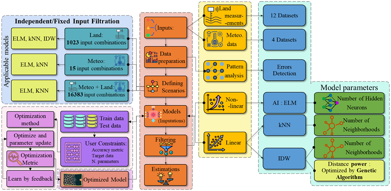
Figure 1. Flowchart of the studied methodology.
To assess the effectiveness of the models and contrast the results, a thorough assessment of the models is carried out utilizing correlation, absolute and relative error, complexity indices, and other visual metrics. The root-mean-square error (RMSE), mean absolute error (MAE), and correlation coefficient (R) are calculated accordingly. Another method for calculating model differences is the Nash-Sutcliffe efficiency (NSE). This index, a normalized method, assesses the residuals' variance with respect to a reference sample. It ranges from –∞ to 1, with 1 being the ideal efficiency/fit. The NSE is, in general, comparable to the R index. However, it assesses the model's effectiveness and performance quality and reflects more precisely the desirable and undesirable aspects of the model under discussion. As a result, it is a useful metric for assessing how well a model performs in comparison to a benchmark model.
where Toi is the ith target variable, and Tmi is the ith modeled target. n is the number of observations.
The study field is located north of the Péribonka River, Saint-Jean Lake, Quebec Province, Canada. The measurement sites extend from 71.9992° to 71.9908° west and from 48.7437° to 48.7540° north. There are a total of 12 measurement sites in the study field. The field and measurement site locations are shown in Figure 2. Because of the large number of missing values in the records of one sensor, and to enable consistent training and testing research hypothesis evaluation, the associated recording is removed from the study datasets. Along with the land measurements, four meteorological (meteo) variables are also measured for the study field. These variables are wind speed (WS), relative humidity (RH), dew, and 2 m air temperatures (DT and AT) for the period of the study. These values are measured on an hourly basis from July to August 2022. The statistical features of the records are shown in Figure 3. The soil matric potential (SMP) was measured continuously with commercial tensiometers (HXM-80, Hortau Inc., Lévis, Québec, Canada) connected to the same ST-4 datalogger. The tensiometers were located at the positions displayed in Figure 3 at a depth of 15 cm below the ground.
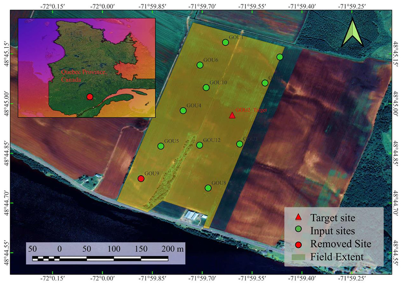
Figure 2. The study field location.
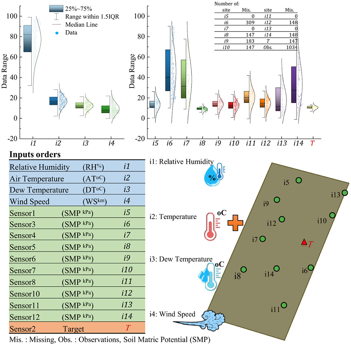
Figure 3. Dataset statistics and representation.
To test the methods presented in this study, an interval in which all time series had reliable values was chosen, and the time steps of missing values were removed from all time series. Therefore, 678 data points for each time series remained. Seventy percent of the datasets were used in the training section, and the remaining thirty percent were used for model evaluation. The size of the test portion was selected based on the maximum rate of missing data and was chosen randomly to simulate real conditions. To choose the target site, the site with the least correlation with the others was selected as the target (T) (Figure 3). The inputs were standardized before being used in the modeling process.
Two general scenarios are defined for imputation, as shown in Figure 1. In the first scenario, the models generate imputations based on all inputs, and each input combination is filtered out after modeling based on the indices. The inputs differ based on the model's structure and the capability of processing inputs of different natures. Therefore, kNN and the ELM modeled the target with 14 inputs, including all meteo and land measurements. On the other hand, gaIDW modeled the target only with land measurements. All combinations of these inputs were analyzed and filtered out, resulting in 16,383 models for the ELM and kNN and 1,023 models for gaIDW. These tasks were performed on a computer with an Intel Core i7 processor and 16 gigabytes of RAM, resulting in 10.83 h of processing time for the ELM, 0.05 h for kNN and 8.42 h for gaIDW.
A graphical representation of the performance of the models is shown in Figure 4 for all generated models. The Violin plots show the distribution and other statistical features of the calculated performance indices (R, MSE, etc.) for the models with independent input data. A violin plot combines aspects of a box plot and a kernel density plot to display model distribution and summary statistics. The width of the violin at different points represents the density or frequency of data values. The high median of the ELM in terms of R and its low values of RMSE, MAE, and NSE suggest better performance for this model, followed by kNN and gaIDW. The ELM was successful in creating relationships among all inputs in all combinations. The bimodal distribution of indices for the ELM and kNN show their higher sensitivity to the inputs compared to that of gaIDW. The uniform and narrower violin body of gaIDW (in RMSE, MAE, and NSE) indicates less variability in the model results. None of the models generated outlier results, indicating the procedure's reliability. According to these plots, the performance of the ELM model was more accurate, followed by kNN and gaIDW, in general.
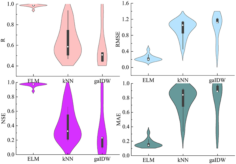
Figure 4. The index ranges for applied models with independent input filtering.
As mentioned earlier, this study aims to assess the possibility of constructing values of different locations in the field with minimum inputs. Therefore, the three subscenarios of modeling with meteo+land inputs, land inputs, and meteo inputs are defined. After assessing all models for different input groups, the best combinations of each group (for instance, 1-input, 2-inputs, …, 14-inputs) are filtered out based on the accuracy indices for each model, and the results of superior combinations are shown in Figure 5. This figure shows the overall performance of the three models with different input combinations. The detailed results are shown in Tables A1–A3. In all three subscenarios, the ELM performed better than kNN and gaIDW. Following relative improvements and alternations of the models for different sub-scenarios are provided. In the chosen 14 superior combinations, the ELM, compared to kNN, is on average more accurate, with R = 37%, RMSE = −74%, MAE = −76%, and NSE = 85%, in the meteo+land subscenario. In the meteo subscenario, the ELM, compared to kNN, is, on average, more accurate with R = 37%, RMSE = −37%, MAE = −45%, and NSE = −130%. In the last subscenario (land inputs), the ELM, compared to kNN, is on average more accurate, with R = 33%, RMSE = −73%, MAE = −76%, and NSE = 79%, and compared to gaIDW, it is more precise, with R = 54%, RMSE = −77%, MAE = −80%, and NSE = 175%. kNN, compared to gaIDW, is also, on average, more accurate with R = 16%, RMSE = −16%, MAE = −17%, and NSE = 54%.
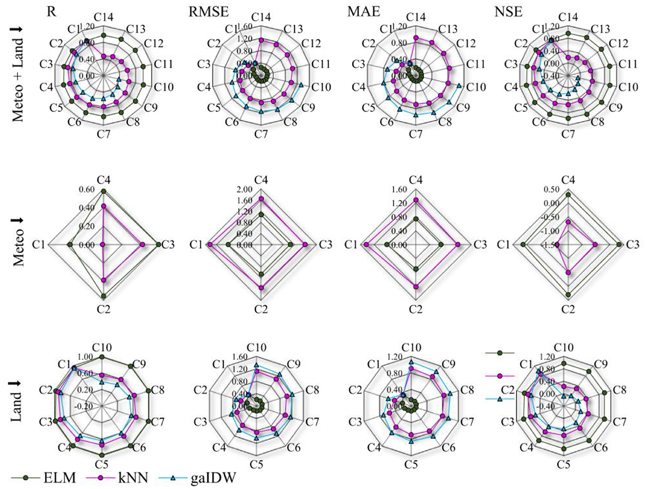
Figure 5. Model results for independent input scenarios, C represents the combinations presented in Tables A1–A3.
The accuracy of estimations for the ELM model increased when increasing the number of inputs to 5, and after that, the accuracy decreased slightly with the increase in the number of inputs. The ELM estimated the target variable most accurately with 5 inputs, having R = 0.992, RMSE = 0.164, MAE = 0.122, and NSE = 0.983. In the first 5 combinations (1-5), only land measurements were involved, and after that, meteo+land combinations yielded slightly more accurate results than the land inputs alone, so they can be used interchangeably and are considerably more accurate than only meteo inputs. The RH, AT, and DT are more involved in the meteo+land combinations than in the other meteo inputs (Table A1).
Conversely, the accuracy of estimations for the kNN model decreased when increasing the number of inputs in both the meteo+land and land subscenarios. The kNN results were obtained using a coefficient of one land input, with a maximum accuracy of R = 0.937, RMSE = 0.455, MAE = 0.336, and NSE = 0.873. The meteo inputs are involved in 3-input combinations and above. With the addition of meteo inputs, kNN generated more accurate estimations compared to only land or only meteo inputs. The RH and WS for meteo inputs were more important input variables than the other two meteo variables in kNN modeling (Table A2). gaIDW also followed the same accuracy decrease pattern as kNN. The best result for this model was obtained with one input, and using all neighbor records decreased the accuracy to half, as demonstrated in the results of Table A3.
The second scenario consists of primary input filtering and use in other models. The processing time for different models was mentioned above, and it was noted that a model such as gaIDW or the ELM could be computationally expensive. Therefore, it is reasonable to use a powerful model to determine the best input combinations and use them in other modeling methods for future applications. The ELM model proved to be robust in finding connections among different inputs in the previous step, while the other models generated relatively naïve results. In this step, the ELM is used as a benchmark model to obtain the primary estimations and filter out combinations. Then, these combinations are used in the other two models to see how much they deviate from the benchmark model and their results in the previous step. The results depicted in Figure 6 reveal that a similar pattern of accuracy changes can be observed in the fixed-input scenario as the number of inputs increases. The gap between the three models is almost the same as the previous one.
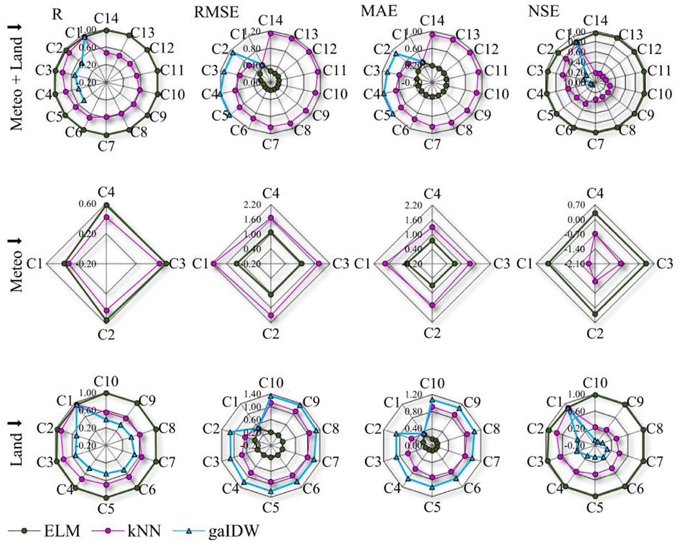
Figure 6. Model results for fixed-input scenarios, C represents the combinations presented in Tables A1–A3.
Following, the comparison of the improvement or degradation of the accuracy of the models relative to each other is presented in terms of percentages of indices' changes. In the filtered combinations, kNN compared to the ELM changed, on average, by R = 53%, RMSE = −76%, MAE = −79%, and NSE = 133% in the meteo+land subscenario. In the meteo subscenario, kNN compared to the ELM changed, on average, by R = 26%, RMSE = −41%, MAE = −49%, and NSE = −123%. In the last subscenario (land inputs), kNN changed compared to the ELM, on average, by R = 38%, RMSE = −74%, MAE = −77%, and NSE = 95%. gaIDW compared to the ELM changed, on average, by R = 72%, RMSE = −78%, MAE = −80%, NSE = 217%. kNN compared to gaIDW also changed, on average, by R = 24%, RMSE = −24%, MAE = −12%, NSE = 63%. These changes are close in RMSE and MAE indices for this modeling scenario compared to the previous one. However, R and NSE have drastic changes in some cases. Figure 7 shows the change rates in the indices when a fixed-input scenario is used. It can be seen that both the kNN and gaIDW models' results differ by a maximum of 20% in R, RMSE, and MAE, except for models with only meteo inputs. However, the efficiency of these models has considerable changes, as it can deviate by up to 40% from the base model in the meteo+land subscenario.
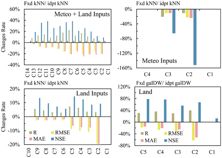
Figure 7. Changes in the indices of models with filtered inputs compared to the same models with independent inputs. Fxd, fixed input models; idpt, independent input models. No column, no changes.
Figure 8 shows the statistical features of the superior models for each modeling method in both scenarios. A powerful model should also be able to reproduce the statistical characteristics of the target series (Zeynoddin and Bonakdari, 2022, 2023). It should be able to estimate the series' mean, median, and distribution, as well as regenerate any outliers. Therefore, box-density plots of the target and models are presented in Figure 8. It can be observed that all models estimated the core features of the target with a high degree of accuracy. The interquartile area and extremes were reproduced with very good accuracy. However, only the ELM model was able to estimate all the outliers of the target series. The scatter plots also show that the chosen models could produce a majority of estimations of the target with 95% intervals.
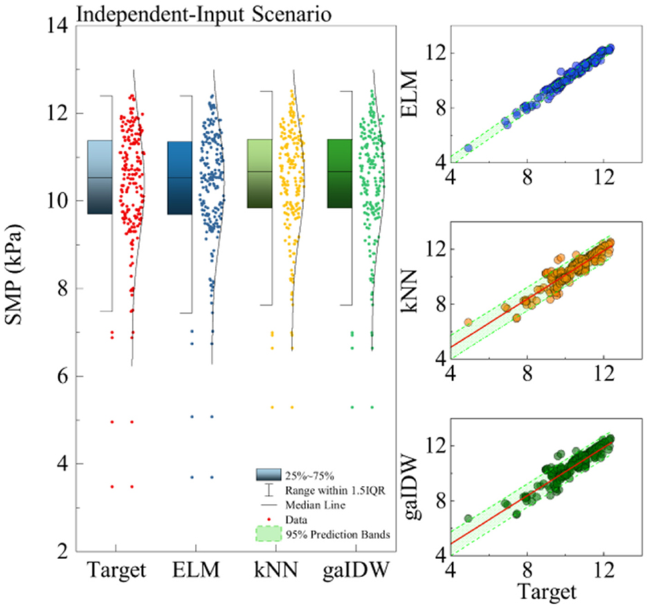
Figure 8. Model statistics for the best results. ELM: Combination (C5): (5,7,8,12,14), kNN (C1): (8), gaIDW (C1): (8).
In all three subscenarios, input 8, which is one of the land inputs, is the main and most important input. This input also has the greatest similarity to the target compared to the others, as shown in Figure 3. If this input was excluded from the input combinations, the best results of the ELM model would be the [1, 3, 7, 11, 13] combination with R = 0.975, RMSE = 0.287, MAE = 0.229, and NSE = 0.949, which is very close to the best result in Table A1. In this combination, two meteo inputs (RH and DT) and three land measurements are involved. With one input, the best results would be [9], with R = 0.655, RMSE = 0.972, MAE = 0.808, and NSE = 0.420, which is considerably lower than the others. With two inputs, the best ELM results would be [7, 12], with R = 0.885, RMSE = 0. 603, MAE = 0. 482, and NSE = 0. 777, and with three inputs, the best ELM results would be [3, 7, 12], with R = 0. 945, RMSE = 0. 418, MAE = 0. 328, and NSE = 0. 893.
The RH and DT meteo input and records at sites 7, 11, 12, and 13 are the most important input variables for estimating the target. For the ELM model to provide the best results with a maximum of 5% difference compared to the best input combination, it needs at least 5 inputs, which can be different combinations of the meteo and land inputs, as shown earlier. With the same exclusion assumption (removing input 8), kNN's best result would be the [4, 5, 9] combination, with R = 0.497, RMSE = 1.151, MAE = 0.930, and NSE = 0.187. Removing input 8 from the combinations greatly affects the results of kNN. Similar to kNN, the gaIDW results would be impacted significantly by removing input 8. The outcome of this model after removing input 8 is R = 0.553, RMSE = 1.219, MAE = 1.032, and NSE = 0.087. This model generates almost identical results for inputs 5, 9, 11, and 13, regardless of the number of inputs or the combination of them.
Using the nearest adjacent sites for data reconstruction is a common approach, and it can be effective in certain cases. The general rule of thumb is based on the assumption that adjacent sites are more likely to have similar characteristics or behavior, which makes them potentially suitable for imputing missing data. However, it is important to note that this rule may not always hold true, and there are several factors to consider when deciding whether to use adjacent sites for data reconstruction, such as spatial relationships, the homogeneity of the study area, temporal relationships, data quality and consistency (Eskelson et al., 2009; Carvalho et al., 2016; Cheng and Lu, 2017; Liu et al., 2020). All these conditions apply to the data used. However, the adjacent sites were less effective than the others in imputing the missing values in this case study. Figure 9 shows the affecting inputs for all three models with and without input 8. This figure shows the relative positions of the inputs to the target.
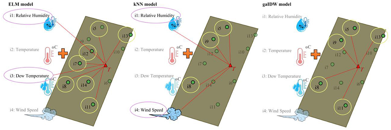
Figure 9. The connections of the most important affecting inputs (main and alternatives) on the target variable.
The application of SMP in precision agriculture, water management, and hydrological studies is extensive. But the challenges in using this parameter and handling UMD are significant. Following, a few studies are presented that encountered UMD. Our findings in the context of these studies, as proper imputation of SMP by proposed methods, could enhance water use efficiency in precision irrigation and hydrological assessments. Borken et al. (2000), while studying the influence of rainfall on distribution in the CH4 oxidation in an ecosystem, found a strong correlation between the variability of this CH4 and SMP. They handled the challenge of UMD by replacing the missing SMP with estimations of the soil water balance model. Using RH and DT meteorological variables or even the rainfall time series and some SMP measurements in the neighborhood, as discussed here, could provide better insight for their study, considering a correlation of 0.89 between parameters. Similarly, when Nzokou et al. (2010) faced the problem of missing and erroneous data while logging SMP for automated irrigation and management of trees, they could compensate the UMD by using logged data by other wired sensors. AI methods' results are dependent on the inputs and their inherent errors. When modeling a soil parameter with these methods, the number of inputs gains importance. So, Cordeiro et al. (2022) could decrease the number of inputs in their model by increasing the accuracy of the imputed features by kNN.
Based on the results of the fixed-input scenario, 20% changes in model outcomes such as R, RMSE, and MSE can be expected. As kNN is considerably faster than the ELM and gaIDW, it can be used as a filtering model to find the best input, and the ELM or other more complex non-linear models can be used to impute the datasets. With this approach, the computational problem can be handled. The limitations of this study can be addressed as follows. The models used in this study are data-driven and are influenced by the quality of the data, the number of inputs, and hyperparameters adjustment, like gaIDW. Accordingly, in case the structure of the time series varies in different timeframes, the results will be affected, specifically in simple-structured models like IDW or kNN. Although the proposed filtering algorithm, as investigating all possible input combinations and filtering superior ones by a fast model and using them in a more complex model like ELM, other machine learning methods or even deep learning methods, is applicable to all types of time series and different structures. Spatial models like gaIDW are also limited to in-situ inputs. This research studied a wide range of different combinations of inputs of different natures. These inputs were data that have been commonly examined in various studies and are readily available. However, there might be other relevant variables that were not considered. Based on the addressed limitations, for future studies, it is suggested that support vector machines, group methods of data handling, or even convolutional neural networks, which are more complicated machine learning methods, be considered as other AI methods in SMP imputation. Therefore, a comparison of different AI methods in SMP estimation in different climatic conditions can also be provided. Adding different inputs to the input set can also expand the search space for the best input combinations, which increases the chance of finding other estimation possibilities. However, based on the findings of this study, exclusively using variables such as meteorological data as input for imputation, which have a different nature than the target variable, does not yield accurate results; instead, they need to be combined with land data to improve accuracy, as was observed in the meteo subscenario. This approach generates more accurate outcomes than only taking land measurements as the inputs.
Water management is vital for precise irrigation guidelines, enhancing potato crop productivity, and optimizing water consumption. Real-time soil matric potential (SMP) can improve water use efficiency. However, the ability to record this variable is constrained, leading to UMD data in the associated time series. In this study, a comparison of three models and the development of an algorithm were investigated, based on which a thorough analysis of inputs was performed to determine the possibility of imputing missing values in datasets with meteorological or field measurements. Four meteorological variables and ten field measurements, constituting 16,383 distinct combinations, were used to reconstruct the missing values. In these scenarios, sole meteorological, sole land, and combinations of both types of variables were investigated. The results of applying the ELM, kNN, and gaIDW in two different scenarios and three subscenarios showed that the ELM model outperformed kNN and gaIDW with 5 inputs consisting of land measurements. Based on a search of the models' results for input alternatives, it was determined that the ELM model requires a minimum of 5 inputs, which can be combinations of RH and DT meteorological variables and land inputs, to achieve optimal results within 5% of the best input combination found earlier. The best kNN outcome was obtained for one land input. Combining meteorological variables as meteo+land inputs, enhanced the model outputs. gaIDW method produced the best results with the same land input as that of kNN and almost identical indices. It was observed that the adjacent sites were not as effective as the others in imputing the missing values, and other input combination possibilities should be investigated. Computational cost is a problem for AI models that was mentioned earlier. To solve this problem, a fast base model can be used to filter the inputs. With this approach, a maximum 20% difference in the results of simple-structured models such as gaIDW and kNN could be expected. However, this issue can be addressed with more complex models, such as stochastic models or other AI models, like group methods of data handling. Exclusively using variables such as meteorological data as input for imputation, which have a different nature than the target variable, does not yield accurate results; instead, they need to be combined with land data to improve accuracy, as was observed in the meteo subscenario.
The raw data supporting the conclusions of this article will be made available by the authors, without undue reservation.
Methodology: HB and MZ. Validation: SG, HB, and MZ. Formal analysis, software, visualization, and investigation: MZ. Resources, conceptualization, project administration, funding acquisition, and data curation: SG. Writing—original draft preparation: SG and MZ. Writing—review and editing and supervision: SG and HB. All authors contributed to the article and approved the submitted version.
The authors declare that the research was conducted in the absence of any commercial or financial relationships that could be construed as a potential conflict of interest.
All claims expressed in this article are solely those of the authors and do not necessarily represent those of their affiliated organizations, or those of the publisher, the editors and the reviewers. Any product that may be evaluated in this article, or claim that may be made by its manufacturer, is not guaranteed or endorsed by the publisher.
The Supplementary Material for this article can be found online at: https://www.frontiersin.org/articles/10.3389/frwa.2023.1237592/full#supplementary-material
Allison, P. D. (2003). Missing data techniques for structural equation modeling. J. Abnorm. Psychol. 112, 545–557. doi: 10.1037/0021-843X.112.4.545
Azari, A., Zeynoddin, M., Ebtehaj, I., Sattar, A. M. A., Gharabaghi, B., and Bonkadari, H. (2021). Integrated preprocessing techniques with linear stochastic approaches in groundwater level forecasting. Acta. Geophys. 6, 472. doi: 10.1007/s11600-021-00617-2
Azimi, H., Bonakdari, H., and Ebtehaj, I. (2017). Sensitivity analysis of the factors affecting the discharge capacity of side weirs in trapezoidal channels using extreme learning machines. Flow Meas. Instr. 54, 216–223. doi: 10.1016/j.flowmeasinst.2017.02.005
Barbulescu, A., Bautu, A., and Bautu, E. (2020). Optimizing inverse distance weighting with particle swarm optimization. Appl. Sci. 10, 2054. doi: 10.3390/app10062054
Bárbulescu, A., Şerban, C., and Indrecan, M.-L. (2021). Computing the beta parameter in IDW interpolation by using a genetic algorithm. Water 13, 863. doi: 10.3390/w13060863
Bennett, D. A. (2001). How can I deal with missing data in my study? Austr. J. Pub. Health 25, 464–469. doi: 10.1111/j.1467-842X.2001.tb00294.x
Bhattacharjee, S., Mitra, P., and Ghosh, S. K. (2014). Spatial interpolation to predict missing attributes in GIS using semantic kriging. IEEE Trans. Geosci. Remote Sensing 52, 4771–4780. doi: 10.1109/TGRS.2013.2284489
Bidwell, V. J. (2005). Realistic forecasting of groundwater level, based on the eigenstructure of aquifer dynamics. Mathematic. Comput. Simulat. 69, 12–20. doi: 10.1016/j.matcom.2005.02.023
Bleidorn, M. T., Pinto, W. P., Schmidt, I. M., Mendonça, A. S. F., and Reis, J. A. T. d. (2022). Methodological approaches for imputing missing data into monthly flows series. Rev. Ambiente Água 17, 1–27. doi: 10.4136/ambi-agua.2795
Bonakdari, H., Moradi, F., Ebtehaj, I., Gharabaghi, B., Sattar, A. A., Azimi, A. H., et al. (2020a). A non-tuned machine learning technique for abutment scour depth in clear water condition. Water 12, 301. doi: 10.3390/w12010301
Bonakdari, H., Qasem, S. N., Ebtehaj, I., Zaji, A. H., Gharabaghi, B., and Moazamnia, M. (2020b). An expert system for predicting the velocity field in narrow open channel flows using self-adaptive extreme learning machines. Measurement 151, 107202. doi: 10.1016/j.measurement.2019.107202
Borken, W., Brumme, R., and Xu, Y.-J. (2000). Effects of prolonged soil drought on CH 4 oxidation in a temperate spruce forest. J. Geophys. Res. 105, 7079–7088. doi: 10.1029/1999JD901170
Carvalho, J. R. P., Nakai, A. M., and Monteiro, J. E. B. (2016). Spatio-temporal modeling of data imputation for daily rainfall series in homogeneous zones. Rev. Bras. meteoRol. 31, 196–201. doi: 10.1590/0102-778631220150025
Chang, C. L., Lo, S. L., and Yu, S. L. (2005). Applying fuzzy theory and genetic algorithm to interpolate precipitation. J. Hydrol. 314, 92–104. doi: 10.1016/j.jhydrol.2005.03.034
Chen, B., Han, M. Y., Peng, K., Zhou, S. L., Shao, L., Wu, X. F., et al. (2018). Global land-water nexus: Agricultural land and freshwater use embodied in worldwide supply chains. Sci. Total Environ. 614, 931–943. doi: 10.1016/j.scitotenv.2017.09.138
Cheng, S., and Lu, F. (2017). A two-step method for missing spatio-temporal data reconstruction. IJGI 6, 187. doi: 10.3390/ijgi6070187
Cordeiro, M., Markert, C., Araújo, S. S., Campos, N. G., Gondim, R. S., Da Silva, T. L. C., et al. (2022). Towards smart farming: fog-enabled intelligent irrigation system using deep neural networks. Future Gen. Comp. Syst. 129, 115–124. doi: 10.1016/j.future.2021.11.013
Di Piazza, A. (2011). The Problem of Missing Data in Hydroclimatic Time Series. Applicationof Spatial Interpolation Techniques to Construct a Comprehensive of Hydroclimatic Data [Thèse de doctorat]. Sicily: IRIS, Université de Palerme.
Dong, Y., and Peng, C.-Y. J. (2013). Principled missing data methods for researchers. Springerplus 2, 222. doi: 10.1186/2193-1801-2-222
Ebtehaj, I., Bonakdari, H., Zaji, A. H., and Sharafi, H. (2019). Sensitivity analysis of parameters affecting scour depth around bridge piers based on the non-tuned, rapid extreme learning machine method. Neural Comput. Appl. 31, 9145–9156. doi: 10.1007/s00521-018-3696-6
Ebtehaj, I., Soltani, K., Amiri, A., Faramarzi, M., Madramootoo, C. A., and Bonakdari, H. (2021). Prognostication of shortwave radiation using an improved no-tuned fast machine learning. Sustainability 13, 8009. doi: 10.3390/su13148009
Enders, C., and Bandalos, D. (2001). The relative performance of full information maximum likelihood estimation for missing data in structural equation models. Struc. Eq. Model. Multidiscip. J. 8, 430–457. doi: 10.1207/S15328007SEM0803_5
Eskelson, B. N. I., Temesgen, H., Lemay, V., Barrett, T. M., Crookston, N. L., and Hudak, A. T. (2009). The roles of nearest neighbor methods in imputing missing data in forest inventory and monitoring databases. Scand. J. Forest Res.arch 24, 235–246. doi: 10.1080/02827580902870490
Evans, S., Williams, G. P., Jones, N. L., Ames, D. P., and Nelson, E. J. (2020). Exploiting earth observation data to impute groundwater level measurements with an extreme learning machine. Remote Sensing 12, 2044. doi: 10.3390/rs12122044
Fountas, S., Carli, G., Sørensen, C. G., Tsiropoulos, Z., Cavalaris, C., Vatsanidou, A., et al. (2015). Farm management information systems: current situation and future perspectives. Comp. Electr. Agric. 115, 40–50. doi: 10.1016/j.compag.2015.05.011
Gholipour, Y., Shahbazi, M. M., and Behnia, A. (2013). An improved version of inverse distance weighting metamodel assisted harmony search algorithm for truss design optimization. Lat. Am. J. Solids Struct. 10, 283–300. doi: 10.1590/S1679-78252013000200004
Godfray, H. C. J., Beddington, J. R., Crute, I. R., Haddad, L., Lawrence, D., Muir, J. F., et al. (2010). Food security: the challenge of feeding 9 billion people. Science 327, 812–818. doi: 10.1126/science.1185383
Huang, G.-B. (2015). What are extreme learning machines? Filling the gap between frank rosenblatt's dream and john von neumann's puzzle. Cogn. Comput. 7, 263–278. doi: 10.1007/s12559-015-9333-0
Huang, G.-B., Zhou, H., Ding, X., and Zhang, R. (2012). Extreme learning machine for regression and multiclass classification. IEEE Trans. Syst. Man. Cybern. B. Cybern. 42, 513–529. doi: 10.1109/TSMCB.2011.2168604
Kamilaris, A., and Prenafeta-Boldú, F. X. (2018). Deep learning in agriculture: a survey. Comput. Electr. Agric. 147, 70–90. doi: 10.1016/j.compag.2018.02.016
Kim, K.-Y., Kim, B.-J., and Yi, G.-S. (2004). Reuse of imputed data in microarray analysis increases imputation efficiency. BMC Bioinf. 5, 160. doi: 10.1186/1471-2105-5-160
Létourneau, G., Caron, J., Anderson, L., and Cormier, J. (2015). Matric potential-based irrigation management of field-grown strawberry: Effects on yield and water use efficiency. Agric. Water Manage. 161, 102–113. doi: 10.1016/j.agwat.2015.07.005
Li, Z., and Wang, P. (2013). “Intelligent optimization on power values for inverse distance weighting,” in 2013 International Conference on Information Science and Cloud Computing Companion (IEEE), Manhattan, NY, 370–375.
Liu, H., Wang, Y., and Chen, W. (2020). Three-step imputation of missing values in condition monitoring datasets. IET Gen. Trans. Distrib. 14, 3288–3300. doi: 10.1049/iet-gtd.2019.1446
Ly, S., Charles, C., and Degré, A. (2011). Geostatistical interpolation of daily rainfall at catchment scale: the use of several variogram models in the Ourthe and Ambleve catchments, Belgium. Hydrol. Earth Syst. Sci. 15, 2259–2274. doi: 10.5194/hess-15-2259-2011
Matteau, J.-P., Célicourt, P., Létourneau, G., Gumiere, T., and Gumiere, S. J. (2021). Potato varieties response to soil matric potential based irrigation. Agronomy 11, 352. doi: 10.3390/agronomy11020352
Matteau, J.-P., Célicourt, P., Létourneau, G., Gumiere, T., and Gumiere, S. J. (2022b). Effects of irrigation thresholds and temporal distribution on potato yield and water productivity in sandy soil. Agric. Water Manage. 264, 107483. doi: 10.1016/j.agwat.2022.107483
Matteau, J.-P., Celicourt, P., Shahriarina, E., Letellier, P., Gumiere, T., and Gumiere, S. J. (2022a). Relationship between irrigation thresholds and potato tuber depth in sandy soil. Front. Soil Sci. 2. doi: 10.3389/fsoil.2022.898618
Molden, D., Oweis, T., Steduto, P., Bindraban, P., Hanjra, M. A., and Kijne, J. (2010). Improving agricultural water productivity: between optimism and caution. Agric. Water Manage. 97, 528–535. doi: 10.1016/j.agwat.2009.03.023
Nzokou, P., Gooch, N. J., and Cregg, B. M. (2010). Design and implementation of a soil matric potential-based automated irrigation system for drip irrigating fraser fir. Hortte 20, 1030–1036. doi: 10.21273/HORTSCI.20.6.1030
Périard, Y., Caron, J., Lafond, J. A., and Jutras, S. (2015). Root water uptake by romaine lettuce in a muck soil: linking tip burn to hydric deficit. Vadose Zone J. 14, vzj2014.10.0139. doi: 10.2136/vzj2014.10.0139
Rekika, D., Caron, J., Rancourt, G. T., Lafond, J. A., Gumiere, S. J., Jenni, S., et al. (2014). Optimal irrigation for onion and celery production and spinach seed germination in histosols. Agronomy J. 106, 981–994. doi: 10.2134/agronj2013.0235
Rouzinov, S., and Berchtold, A. (2022). Regression-based approach to test missing data mechanisms. Data 7, 16. doi: 10.3390/data7020016
Tipton, J., Hooten, M., and Goring, S. (2017). Reconstruction of spatio-temporal temperature from sparse historical records using robust probabilistic principal component regression. Adv. Stat. Clim. Meteorol. Oceanogr. 3, 1–16. doi: 10.5194/ascmo-3-1-2017
Tonini, F., Dillon, W. W., Money, E. S., and Meentemeyer, R. K. (2016). Spatio-temporal reconstruction of missing forest microclimate measurements. Agric. Forest Meteorol. 218-219, 1–10. doi: 10.1016/j.agrformet.2015.11.004
Troyanskaya, O., Cantor, M., Sherlock, G., Brown, P., Hastie, T., Tibshirani, R., et al. (2001). Missing value estimation methods for DNA microarrays. Bioinformatics 17, 520–525. doi: 10.1093/bioinformatics/17.6.520
Wolfert, S., Ge, L., Verdouw, C., and Bogaardt, M.-J. (2017). Big data in smart farming – a review. Agric. Syst. 153, 69–80. doi: 10.1016/j.agsy.2017.01.023
Yaseen, Z. M., Deo, R. C., Ebtehaj, I., and Bonakdari, H. (2018). “Hybrid data intelligent models and applications for water level prediction,” in Handbook of Research on Predictive Modeling and Optimization Methods in Science and Engineering, eds. I. Giannoccaro, D. Kim, S. Sekhar Roy, T. Länsivaara, R. Deo, and P. Samui (London: IGI Global), 121–139.
Yozgatligil, C., Aslan, S., Iyigun, C., and Batmaz, I. (2013). Comparison of missing value imputation methods in time series: the case of Turkish meteorological data. Theor. Appl. Climatol. 112, 143–167. doi: 10.1007/s00704-012-0723-x
Zeynoddin, M., and Bonakdari, H. (2022). Structural-optimized sequential deep learning methods for surface soil moisture forecasting, case study Quebec, Canada. Neural. Comput. Applic. 10, 19895–19921. doi: 10.1007/s00521-022-07529-2
Zeynoddin, M., and Bonakdari, H. (2023). A comparative analysis of SMAP-derived soil moisture modeling by optimized machine learning methods: a case study of the Quebec province. ECWS-7 2023 37, 1–4. doi: 10.3390/ECWS-7-14183
Zeynoddin, M., Bonakdari, H., Azari, A., Ebtehaj, I., Gharabaghi, B., and Madavar, H. R. (2018). Novel hybrid linear stochastic with non-linear extreme learning machine methods for forecasting monthly rainfall a tropical climate. J. Environ. Manage. 222, 190–206. doi: 10.1016/j.jenvman.2018.05.072
Keywords: imputation, machine learning, modeling, hydro-informatics, soil matric potential, water management
Citation: Zeynoddin M, Gumiere SJ and Bonakdari H (2023) Enhancing water use efficiency in precision irrigation: data-driven approaches for addressing data gaps in time series. Front. Water 5:1237592. doi: 10.3389/frwa.2023.1237592
Received: 09 June 2023; Accepted: 31 July 2023;
Published: 22 August 2023.
Edited by:
Georgia A. Papacharalampous, National Technical University of Athens, GreeceReviewed by:
Francesco Granata, University of Cassino, ItalyCopyright © 2023 Zeynoddin, Gumiere and Bonakdari. This is an open-access article distributed under the terms of the Creative Commons Attribution License (CC BY). The use, distribution or reproduction in other forums is permitted, provided the original author(s) and the copyright owner(s) are credited and that the original publication in this journal is cited, in accordance with accepted academic practice. No use, distribution or reproduction is permitted which does not comply with these terms.
*Correspondence: Silvio José Gumiere, U2lsdmlvLUpvc2UuR3VtaWVyZUBmc2FhLnVsYXZhbC5jYQ==
Disclaimer: All claims expressed in this article are solely those of the authors and do not necessarily represent those of their affiliated organizations, or those of the publisher, the editors and the reviewers. Any product that may be evaluated in this article or claim that may be made by its manufacturer is not guaranteed or endorsed by the publisher.
Research integrity at Frontiers
Learn more about the work of our research integrity team to safeguard the quality of each article we publish.