 Marthe Grønlie Guren
 François Renard
 Catherine Noiriel
- 1Departments of Geosciences and Physics, The Njord Centre, University of Oslo, Oslo, Norway
- 2ISTerre, University Grenoble Alpes, University Savoie Mont Blanc, University Gustave Eiffel, CNRS, IRD, Grenoble, France
- 3Géosciences Environnement Toulouse, Observatoire Midi-Pyrénées, Université Paul Sabatier, CNRS, IRD, CNES, Université de Toulouse, Toulouse, France
We provide a detailed 3D characterization of the geometry evolution and dissolution rate mapping at the surface of four carbonate samples, namely a calcite spar crystal, two limestone rock fragments, and an aragonite ooid, using time-lapse X-ray micro-tomography during dissolution experiments at pH 4.0. Evaluation of the retreat and mapping of the reaction rates at the whole surface of the samples reveals a large spatial variability in the dissolution rates, reflecting the composition and the specific contributions of the different regions of the samples. While crystal edges and convex topographies record the highest dissolution rates, the retreat is slower for flat surfaces and in topographic lows (i.e., concave areas), suggesting surface-energy related and/or diffusion-limited reactions. Microcrystalline aragonite has the highest rate of dissolution compared to calcite. Surprisingly, rough microcrystalline calcite surface dissolves globally more slowly than the faces of the calcite spar crystal. The presence of mineral impurities in rocks, through the development of a rough interface that may affect the transport of species across the surface, may explain the slight decrease in reactivity with time. Finally, a macroscopic stochastic model using the set of detachment probabilities at corner, edge, and face (terrace) sites obtained from kinetic Monte Carlo simulations is applied at the spar crystal scale to account for the effect of site coordination onto reactivity. Application of the model to the three other carbonate samples is discussed regarding their geometry and composition. The results suggest that the global dissolution process of carbonate rocks does not reflect only the individual behavior of their forming minerals, but also the geometry of the crystals and the shape of the fluid-mineral interface.
1. Introduction
One of the most important geochemical reactions occurring at conditions of Earth's surface is the dissolution of sedimentary carbonates, where the most abundant minerals are calcite, dolomite, aragonite, and high-Mg calcites (Morse and Arvidson, 2002). Although the dissolution of carbonate minerals has received considerable attention, the upscaling of reaction rates determined from laboratory experiments to natural settings remains to be fully understood (Morse and Arvidson, 2002; Noiriel et al., 2020).
Several techniques have been developed over the past century to derive dissolution rates from batch or flow-through experiments in the laboratory (Morse and Arvidson, 2002). Direct measurements of the surface retreat perpendicularly, i.e., normal to the mineral surface, provide dissolution rates at micrometer to nanometer scales on face-oriented single crystals or polycrystalline aggregates. Such measurements rely on imaging techniques such as atomic force microscopy (Hillner et al., 1992; Stipp et al., 1994; Jordan and Rammensee, 1998; Shiraki et al., 2000; Emmanuel, 2014), vertical scanning interferometry (Fischer and Luttge, 2007; Smith et al., 2013; Pedrosa et al., 2021), confocal profilometry (Godinho et al., 2012), X-ray reflectivity (Fenter et al., 2000), digital holographic microscopy (Brand et al., 2017), or X-ray microscopy (Laanait et al., 2015). Determination of dissolution rates from surface retreat has the advantage of providing accurate measurements of mineral reactivity, as there is no need of normalization to the specific surface area, a parameter difficult to assess practically (Noiriel and Daval, 2017). However, application of these methods is often restricted to small surface areas, and require the surface to be well-cleaved or polished, and as flat as possible (Noiriel et al., 2020). In contrast, the fluid-mineral interfaces depicted in porous or fractured media are often curved or exhibit roughness at several scales. Non-invasive and non-destructive 4D X-ray micro-tomography (XMT) imaging has recently emerged as a useful technique to track through time the geometrical complexity of the interface during mineral dissolution (Noiriel et al., 2019, 2020; Yuan et al., 2019, 2021; Noiriel and Soulaine, 2021; Noiriel and Renard, 2022). A whole crystal can be imaged, including corners and edges, whose reactivity might differ from the well-cleaved faces. Contribution of etch pits, grain boundaries and other defects which have a significant contribution to the reaction rate variability can also be evaluated. Geological material and rock fragments of any geometry can additionally be studied. XMT imaging produces routinely data sets of several gigabytes in size. Sample volume is commonly in the order of billion voxel elements, for a fluid-solid interface in the order of million pixel elements, thus providing a large amount of data points for statistical analysis during geochemical processes.
Stochastic modeling of kinetic processes has emerged in the mid-1970s (Gilmer, 1977, 1980; Lasaga and Blum, 1986). Modeling can be useful to decipher the dissolution mechanisms at play at the atomic scale (de Leeuw et al., 1999; Lasaga and Luttge, 2001; Spagnoli et al., 2006; Lardge et al., 2010; Wolthers et al., 2012; Kurganskaya and Luttge, 2016; Kurganskaya and Churakov, 2018; Kurganskaya and Rohlfs, 2020), like etch pit formation at dislocation outcrops, and to compare modeled and measured dissolution rates (Kurganskaya and Luttge, 2016). Among the methods, kinetic Monte Carlo (kMC) modeling has been widely used for the study of crystal dissolution kinetics and surface reactivity (Liang et al., 1996; Bandstra and Brantley, 2008; Fischer et al., 2018; Andersen et al., 2019; Luttge et al., 2019), principally using simple Kossel crystals (de Assis and Aarao Reis, 2018; Carrasco and Aarão Reis, 2021) even if more complex geometries have also been investigated (Zhang and Lüttge, 2007; Kurganskaya and Luttge, 2016). kMC simulations allow for observation of the dynamics of surface topography and calculation of the dissolution rates (Wehrli, 1989; Kurganskaya and Luttge, 2016). The Transition State Theory (Eyring, 1935) adapted to the terrace-ledge-kink model (Kossel, 1927) intends to simulate the time evolution of mineral dissolution by linking the reaction rate to a probability of detachment at the surface. The kMC method replaces various kinetic rates by probabilities, with bond-breaking probabilities related to the activation energy for chemical bond hydrolysis. The detachment rate of an element with coordination n, rn (s−1), is derived from the standard model of thermally activated dissolution (Lasaga and Blum, 1986; McCoy and LaFemina, 1997) and written as:
where ν is the pre-exponential or frequency factor characterizing the interaction with water molecules (whose usually adopted value is 10−12 s−1), R is the gas constant (8.314 J·mol−1·K−1), T is the temperature (K), and Eb is interpreted as a bond-breaking activation energy. The standard model of thermally activated dissolution assumes that the bond-breaking activation energies are additive over the nearest neighbors, i.e., nEb, and Equation (1) resumes to:
with ϵ = exp(−Eb/RT). High rates of dissolution can be related to sites of higher surface energy, whereas low dissolution rates are related to sites of lower energy. Consequently, a rate set r = {rn} that depends only on the site coordination can be derived for a crystal, as a value of ϵ. The very low bond-breaking probabilities during geochemical processes would make the kMC simulation too time-consuming, so that a scaling factor is applied to the set of probabilities, P = {Pn}, associated to the rate set {rn}. In the divide-and-conquer algorithm (Meakin and Rosso, 2008), for instance, the surface elements are listed according to their detachment probability Pi, e.g., in relationship with their bond type or coordination number. The set of probabilities P = {P1, P2, ..., Pi} is then normalized to a value close to unity, so that an element is removed at each iteration or so. Then, the time and the list of elements are updated before the next iteration. On the long term, the surface geometry evolution is found to be highly dependent to the set of probabilities derived from the rate set.
Nevertheless, kMC simulations remain time-consuming, and a current restriction of the models is their limitation to handle large-size systems. As a result, simulations are often restricted to small crystal surface portions, or Kossel crystals of size below 1,000 × 1,000 × 1,000 elements. Using an edge length of 0.394 nm to reproduce the lattice parameters and molar volume of calcite, such domain size represents a microscopic volume of about 400 × 400 × 400 nm, a scale far below the size of macroscopic crystals in nature. A mm-size crystal would require a domain of about 2.5 106 × 2.5 106 × 2.5 106 elements. As a consequence, kMC simulations of macroscopic crystals remain elusive.
Upscaling of kMC simulations to large-size crystals is a real challenge, as the proportion of face (terrace), edge and corner (kink) elements in a Kossel crystal is also strictly proportional to the size of the system. Indeed, a Kossel crystal of side a has initially eight corners, 12·(a-2) edges, and 6·(a-2)2 face elements. Therefore, both the probability of detachment of the various elements and the consequent geometry evolution depend on the initial crystal size. Consequently, although the value of ϵ is not size-dependent, the resulting converged set of probabilities is clearly dependent on the size of the crystal. Nevertheless, a few authors have proposed to upscale kMC simulations to larger scales (Rohlfs et al., 2018; Carrasco and Aarão Reis, 2021). In particular, for far-from-equilibrium calcite dissolution in neutral to alkaline solution, Carrasco and Aarão Reis (2021) have extrapolated macroscopic rates at room temperature from kMC simulations run at high temperature. The authors observed in their kMC simulations at high temperature, i.e., at high values of ϵ, the existence of a steady-state kinetic regime on the long term. From that steady-state regime, they derived macroscopic rates at ambient temperature at which the bond-breaking activation energy Eb and ϵ are far lower. However, calcite is unlikely to be stable at such high temperatures, and it is not possible to verify that the geometry evolution would be similar in such different conditions.
On the other hand, other stochastic modeling methods, like the cellular automata (Jansen, 2012), have been developed to overcome the system-size restrictions. In that case, several listed elements can be removed from the mineral surface at every iteration following a set of defined probabilities. Overall, the description is less mechanistic but has the advantage of not being restricted in term of system size or time for simulations.
In this article, we investigate the surface reactivity during dissolution at pH 4.0 of four, mm-scale, natural calcium carbonate samples, namely a calcite spar crystal, a fragment of micritic limestone, a fragment of dolomitic limestone and an ooid of aragonite. We provide direct measurement of the surface retreat rate using time-lapse 3D XMT (i.e., 4D XMT), and quantify the heterogeneous distribution of the dissolution fluxes of the samples reacted through time from between 2.1 and 5.6 millions of data points analyzed at each time step at their surface. These data points and the XMT geometries retrieved from the experiments are used to constrain a stochastic model for calcite dissolution at the macroscale. Sets of converged probabilities are derived from kMC simulations on a Kossel crystal and implemented at larger scale to model dissolution of the samples. The dissolution process of the calcite crystal in the experiments helps to constrain the model, which is next applied to the other samples. The main objective is to track the whole topography evolution of the fluid-mineral interface at different time intervals in order to evaluate the contribution of the surface topography (i.e., roughness, and convex to concave surface areas) and geometrical features (i.e., crystal face, edges, and corners) to the reaction rate distribution. We demonstrate quantitatively how the crystal edges, interface shape, and surface roughness play a major role in the dissolution process, and discuss also the limitation of the model on geometries derived from XMT.
2. Materials and methods
2.1. Materials and sample preparation
Four types of carbonate samples (Figure 1) were prepared for the dissolution experiments: a calcite spar crystal (CALSPAR), a microcrystalline limestone (CALMICR), a microcrystalline dolomitic limestone (CALDOL), and an aragonite ooid (ARAGOID). The samples differ by their shape, size, surface roughness, and mineralogical composition.
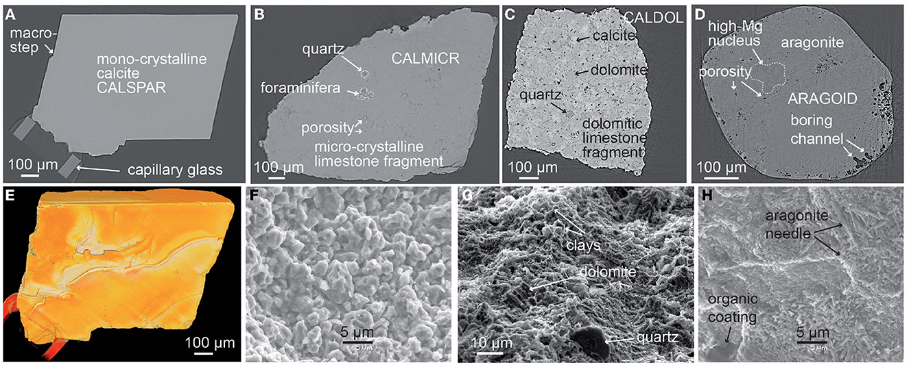
Figure 1. Description of the four samples. (A–D) XMT cross-sections of the samples before experiment, with (A) calcite spar (CALSPAR), (B) microcrystalline limestone sample (CALMICR), (C) dolomitic limestone sample (CALDOL), and (D) aragonite ooid (ARAGOID). (E) XMT 3D view of the calcite spar crystal before experiment. (F–H) SEM observations at the surface of similar specimens of (F) aragonite, (G) microcrystalline limestone, and (H) dolomitic limestone after 18 or 29 h of dissolution under the same experimental conditions.
The calcite crystal CALSPAR (Figures 1A, E) has a length of about 0.5 mm, and was obtained after crushing and sieving of a cm-size single spar crystal. The crystal was not polished before experiment, so that the faces exhibit various macro-features such as macro-steps and rippled surface patterns, which were inherited from the breaking and size reduction of the original calcite sample. The dissolution behavior of this crystal has been described in details in Noiriel et al. (2019). The other three samples described below are original data.
The microcrystalline calcite-rich rock sample CALMICR (Figure 1B) has a pyramidal shape, and was produced after breaking a micritic limestone of lower Cretaceous age. A few microfractures intersect the surface. The rock is dominated by fine-grained calcite (micrite) with an anhedral texture (Periere et al., 2011). No clay was detected with X-ray diffraction (XRD), although sporadic clay patches have been noticed with XMT and scanning electron microscopy (SEM) imaging of the rock (Noiriel and Deng, 2018). A few quartz particles of 5–20 μm in size (~0.5 wt%) are also noticed, as a few dissolved tests of foraminifera (Globigerina) of ~100 μm in size. The sample is a low permeability and porosity limestone, although some μm-size pores are visible in the matrix.
The microcrystalline calcite- and dolomite-rich rock sample CALDOL (Figure 1C) has a cubic shape, and was obtained after crushing a dolomitic limestone of Upper Jurassic age. The surface of the fragment is initially rough and results from the mechanical behavior of the mineral assemblage during fracturing. A few microfractures also intersect the surface. The rock composition given by XRD analysis is about 50 wt% calcite and 50 wt% dolomite, with a minor amount of quartz, clays, and K-feldspar. The carbonate matrix contains a microsparitic cement of calcite and dolomite, dispatched as patches of about 10.5 μm in size. Pores in the range 0–20 μm (4 μm in average) are also identified with XMT imaging. The macro-porosity is 2%.
The spheroidal aragonite ooid ARAGOID (Figure 1D) has a diameter of about 700 μm, and comes from present oolitic sand sampled on the seabed in Bahamas. SEM coupled to energy dispersive X-ray spectroscopy (SEM-EDS) reveals that the ooids consist of high-Mg carbonate nuclei (foraminifera fragments) surrounded by sub-micrometric needle-shaped acicular crystals of aragonite. The surface of the ooids exhibits several boring channels and organic coating marks are visible. Bulk analysis using inductively coupled plasma-mass spectroscopy (ICP-MS) after acid attack gives the following major elementary chemical composition: Ca 37.9 wt%, Si 1.4 wt%, Sr 1.2 wt%, Mg 0.3 wt%, Ba 0.2 wt%, others <0.05 wt%.
2.2. Dissolution experiments
The samples were glued on glass capillary tubes (Hilgenberg, 400 μm O.D.) using epoxy resin, which covers their bottom part creating a mask that preserves it from dissolution. Whereas, only a small corner region of the CALSPAR sample is glued, a larger portion of the CALMICR, ARAGOID, and CALDOL surfaces are covered by glue. Three of the samples, CALSPAR, CALMICR, and ARAGOID, were reacted together in a mixed-flow reactor during 12 h, to exclude variations due to extrinsic experimental factors. The sample CALDOL was dissolved in a separate reactor for 12.8 h to avoid potential contamination of the other samples by Mg2+ ions. The experiments were performed at ambient temperature (25±2 °C) under atmospheric pressure. The inlet solution was prepared with deionized water (18.2 MΩ·cm−1) and 0.01 M NaCl and the pH was adjusted to 4.0 ± 0.1 using analytical grade HCl. At low pH, the dissolution rate is almost directly proportional to the H+ concentration (Sjöberg and Rickard, 1984), and is high enough to quantify volumes changes by XMT imaging over a few hours. The reactors have a volume of 160 mL and were filled with the inlet solution. The flow rate was set equal to 8 cm3·h−1 and the stirring rate was set equal to 400 rpm during the experiments to homogenize the solution around the samples and impose far-from-equilibrium conditions. Because of the high fluid volume to mineral surface ratio, the calcium concentration in the aliquots collected during the experiments and analyzed by ICP-MS remains below 2.9×10⁻⁵ M over the course of the experiment. The corresponding saturation ratio (Ω) with respect to calcite and aragonite, calculated with Phreeqc v3.0 (Parkhurst and Appelo, 2013) using the Phreeqc database, remained below 10−9 throughout the experiments, thus excluding any measurable effect of fluid chemistry or saturation index evolution on the dissolution rates. However, due to the high ionic force of the solution, the concentrations of Ca2+ and Mg2+ measured in the aliquots are not accurate enough to properly evaluate the mass balance.
2.3. 4D imaging with X-ray micro-tomography
The four samples were imaged before the reaction (t0) and at five time steps (t1-t5) during the dissolution experiment using 3D XMT at the TOMCAT beamline (Stampanoni et al., 2006), Swiss Light Source (Paul Scherrer Institute, Switzerland). A total of 24 data sets were collected. Each data set is composed of 1701 radiographs collected over a 180° rotation range. Each radiograph was recorded with a monochromatic and parallel beam at the energy of 20 keV and an exposure time of 200 or 250 ms. After penetration of the samples, the X-rays were converted into visible light with a LuAG:Ce scintillator. The visible light was magnified using either a × 10 or a × 20 magnification diffraction-limited microscopy optics and recorded with a sCMOS camera of 2,560 × 2,160 pixels. The resulting pixel size is 0.65 μm for the CALSPAR, CALMICR, and CALDOL samples, and 0.325 μm for the ARAGOID sample. Volume reconstructions were performed from the radiographs corrected from flat field and background noise using an algorithm based on the Fourier transform method (Marone and Stampanoni, 2012).
After reconstruction of the 3D images, image processing was carried out with Avizo® software on data sets of 1,700 × 500 × 1,300 (CALSPAR), 1,700 × 500 × 1,300 (CALMICR), 1,450 × 1,400 × 1,100 (CALDOL) or 1,910 × 1,600 × 1,400 (ARAGOID) voxels. First, the 3D grayscale volumes were normalized, converted to 8-bit integers, and denoised with a 3D median filter using a kernel size of 3 × 3 × 3 voxels. Then, the samples were registered in the same coordinate system, using either the capillary glass and chemically inert masked area (CALSPAR) or the internal structures (CALMICR, CALDOL, and ARAGOID) as landmarks. Data were segmented using either a threshold value halfway between the two maximum peaks for air and calcite (CALSPAR) or a region growing algorithm (CALMICR, CALDOL, and ARAGOID) to provide a discretized geometry of the solid materials (i.e., crystal, rock sample, and ooid). After segmentation, the solid objects, i.e., samples and capillary glass, were labeled to separate and remove the capillary glass from the images. For ARAGOID, CALDOL, and CALMICR samples, the internal non-connected porosity was also filled. The sample volumes, Vsample, are calculated from the number of solid voxels, nsol: Vsample = nsol × Vvoxels, where Vvoxel is the volume of a voxel. The samples surface areas, Ssample, are calculated from the number of solid-air pixel interfaces, nsol−fluid: Vsample = nsol−fluid×Spixel, where Spixel is the surface area of a pixel. The non-reactive volumes and surface areas in the glue are evaluated for each sample and subtracted from the calculations. Complementary to XMT, the surface of the samples or of similar specimens (starting or dissolved material) was also observed using SEM to characterize the surfaces at higher resolution.
2.3.1. Global dissolution rate
The global dissolution rate (mol·s−1) of the samples is calculated after segmentation of the XMT data sets based on the changes in sample volume (Noiriel et al., 2020):
where dVsample is the change in sample volume (m3), Δt is the time interval between successive XMT scans, and νcal is the molar volume of calcite or aragonite (m3·mol−1). The rate (mol·m−2·s−1) can be normalized to the surface area in contact with the fluid:
where is the average surface area between two time intervals as determined by XMT. However, since the samples are partially covered by glue, normalization of the dissolution rate by the total surface area induces a bias, because a non-negligible fraction of the surface is non-reactive for samples CALMICR, CALDOL, and ARAGOID. This point is discussed later in the manuscript.
2.3.2. Mapping of the local dissolution rate at the sample surface
We calculate the local dissolution rate (μm·h−1) at any reactive element (i.e., fluid-solid pixel interface) of the sample surface by calculating the surface retreat after each dissolution stage (Noiriel et al., 2019). The surface retreat is the distance at two time steps calculated normal to the closest surface. Practically, the 3D Euclidean distance maps (Akmal Butt and Maragos, 1998; Russ, 2011) inside the samples are computed at t0. Consequently, each voxel inside an unreacted sample is labeled with the distance to its nearest boundary voxel, starting from the position of the unreacted fluid-solid interface. The distance transform corresponds to a quasi-uniform scaling of the samples. Combining the distance map with the position of the fluid-solid interfaces at each time step of the experiment, ti, gives the surface retreat of the samples normal to the surface of the unreacted samples, as illustrated in Figure 2. In this case, the rate is determined in the interval ti-t0, the initial state being used as a reference for all the calculations. It is worth mentioning that the deep pores connected to the surface as well as the presence of micro-fractures or internal, non-connected pores, may lead to an overestimation of the surface retreat. Nevertheless, these very local phenomena are negligible when considering the large number of data points used to calculate the dissolution rates.
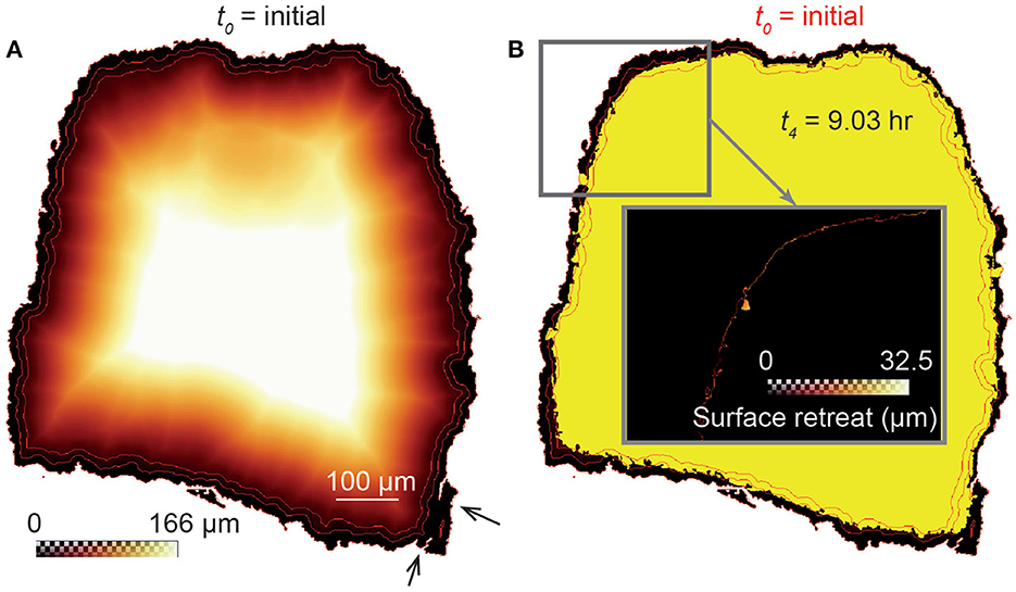
Figure 2. Schematic view (2D cross-section) of the distance transform procedure to calculate the surface retreat between two stages of dissolution. (A) 3D Euclidean distance map inside the unreacted sample CALDOL, which represents the shortest distance of each voxel inside the rock fragment to the fluid-surface interface at t0. Distance contours of 0, 15, and 30 pixels (red lines) are shown to highlight a quasi-uniform scaling of the grain. The black arrows point to micro-fractures that affect the distance map calculation locally. (B) Combining the distance map with the XMT image at t4 (yellow) gives the retreat at the sample surface (see details in the insert).
In addition, we explored the temporal evolution of the dissolution rates. The distance map procedure is repeated for the volumes at t2 and t4, so that temporal evolution of the reaction rate can be followed in the intervals t0-t3, t2-t4, and t3-t5, three time intervals quite comparable with a median value of 6 h.
Then, the local dissolution rates normal to the sample surface are calculated according to:
with Ifs the fluid-mineral position vector, and n the normal to the sample surface; the product Ifs·n is the surface retreat, i.e., the distance normal to the reference surface. The voxels belonging to the unreactive interface, i.e., the epoxy-glued surface or the non-reactive minerals, are superimposable with time, and their retreat is zero. The areas containing glue are excluded from the calculation of the average reaction rate determined from surface retreat, (nm·s−1 or μm·h−1):
with nsol−fluid is the number of reactive voxels at the fluid-solid interface, i.e., for which the retreat rate is non-zero. The average dissolution rate normalized to the surface area, (mol·m−2·s−1) can also be calculated (Arvidson et al., 2004):
It is also possible to determine the dissolution rate of specific faces or areas by averaging the local dissolution rates from volumes of interest (VOIs) defined in these areas.
2.4. Stochastic model for dissolution
Dissolution of a crystal in a far-from-equilibrium solution can be modeled by an irreversible detachment of sites from the mineral surface. We have designed a simplified stochastic model at the macroscopic scale where the basis element is the voxel (of 0.325 or 0.65 μm of side). The model is built such that the sample geometry is defined by the XMT volumes at t0 after segmentation, where the fluid phase is set to 0 and the solid phase to 1. The non-reactive voxels (i.e., the glued part), when identified, are set to 2 using a mask. It is worth mentioning that the glued part of sample ARAGOID is irregular and cannot be masked in a simple way on the 3D volumes, but the spherical symmetry of the sample should not alter much the shape of the modeled rate distribution. Each voxel site at the fluid-solid interface is classified as either a corner, edge, or face element based on the number of nearest solid neighbors (n): one-bonded sites (n=1), two-bonded sites (n=2), corners (n=3), edges (n=4), faces (n=5), or solid bulk (n=6). For simplicity, all voxels with a coordination n=1 or n=2 are considered as corner elements. Corner, edge, and face elements form three groups of Nc, Ne, and Nf elements, respectively.
The aim of the stochastic modeling is to test the ability of the model to reproduce the observation that the crystal edges and corners dissolve faster than faces, or that convex surface dissolves faster that concave surface, in relationship with the coordination of corner, edge and face (i.e., terrace) elements at the microscopic scale. The stochastic model is designed to handle large-size systems, and the modeling procedure is divided in two stages. First, a fixed normalized set of probabilities is derived from kMC simulations at the nm-scale (see Section 2.4.2) and we show that the stochastic model can be effectively parameterized by kMC simulation results. Second, the simulation is run on the mm-size sample geometries.
The stochastic model developed in this study has the advantage to be constrained by the experimental results, i.e., the geometries obtained from XMT at the different time steps and the retreat distribution at the fluid-mineral or fluid-rock interface. Especially, the frequency factor or the activation energy for bound hydrolysis Eb (Equation 1), two parameters whose value is still discussed in kMC simulations (Ackerer et al., 2021), do not need to be known a priori. The setting of a physical time increment at each iteration is also unnecessary. The approach is however less mechanistic compared to kinetic Monte Carlo modeling. Dissolution remains treated as a stochastic process, but it does not require bond-breaking activation energies to be specified. In addition, the approach assumes a scale-dependent behavior for dissolution at faces, edges, and corners in between the microscopic and crystal scales, which remains to be fully demonstrated. However, the 3D XMT geometries serve to constrain and validate modeling at the macroscopic scale, and such a modeling approach offers the capacity to deal with large volume systems.
2.4.1. Sample-scale stochastic simulation procedure
The corner, edge and face elements are divided into three lists: {c, e, f}. We use the normalized set of probabilities provided by kMC simulations on the long term (see Section 2.4.2) as input in the macroscopic stochastic model:
where j is the iteration number and the symbol stands for the normalized probability:
so that the sum of is equal to 1; i represents the class of corner, edge or face elements and Pi is their probability of detachment. At each iteration, a list is randomly chosen based on , and all the voxels belonging to the class are removed at the sample surface, except the non-reactive voxels which do not participate to the reaction, although they are accounted for in the determination of the coordination of the dissolving voxels. The number of removed corner, edge and face elements is determined, and the next iteration starts.
2.4.2. Obtaining dissolution probabilities from kinetic Monte Carlo simulations
The set of probabilities used in the sample-scale stochastic model, , is obtained from kMC simulations. First, we ran kMC simulations on a 100 × 100 × 100 Kossel crystal. The algorithm used is the divide-and-conquer algorithm, whose details can be found in Meakin and Rosso (2008). The corner, edge, and elements are first identified and listed. Each list contains a total of surface sites:
An initial set of probabilities derived for a given value of ϵ is provided: P(j = 0)={Pc, Pe, Pf}. Assuming that all elements in each list have the same dissolution rate, the probability of choosing a list depends on the number of elements in each list. The set of probabilities is also normalized to 1, and becomes:
One of the list is randomly chosen based on this probability set, and one element in the list is randomly removed. Both the lists and the set of probabilities are updated before the next iteration j.
Kinetic Monte Carlo simulations were run on the Kossel crystal until 50% of the volume is removed, i.e., 500,000 iterations. Three different values of ϵ (ϵ = 0.001, 0.01 and 0.1) in Equation (2) were first used to test the kMC model against our macroscopic stochastic model on the crystal geometry evolution (Supplementary Figures 1–3). In the kMC simulations, the size of the Kossel crystal is about 400 × 400 × 400 nm, while in the macroscopic stochastic model, the size of the Kossel crystal is 65 × 65 × 65 μm. The corresponding sets of probabilities are in the range of those chosen by Carrasco and Aarão Reis (2021) to model calcite dissolution in neutral to basic conditions. Although the pH conditions explored in their article differ from the present study, the range of macroscopic dissolution rates obtained by Colombani (2016) in the corresponding experiments, i.e., 0.5–6 10−6 mol·m−2·s−1, is close to the range of rates determined in the present study. It corresponds to a value of ϵ to describe the dissolution mechanism of 1.4 10−3 (Carrasco and Aarão Reis, 2021). Compared to Equation (2), Carrasco and Aarão Reis (2021) used a slightly different formalism to parameterize the dissolution rates at corner, edge, and face sites:
where m=n for a coordination n=3 and n=4, and 5<m<6 for n=5. Taking m>n for cleaved calcite surface results in decreasing the reactivity of the faces.
The initial sets of probabilities P(j = 0) provided to kMC simulations for each list of elements converge to given sets of probabilities on the long term, i.e., for iteration j>>0) (Supplementary Figures 1a–3a). Thus, the long-term sets of probabilities are expected to apply at the macroscopic scale.
2.4.3. Model calibration at the sample scale
Application of the converged sets of probabilities obtained from kMC simulations in the stochastic model at the macroscopic scale leads to the geometries observed in Supplementary Figures 1c–3c. The stochastic model is first calibrated based on the experimental results obtained for sample CALSPAR. The value of ϵ was refined to best match the geometry evolution of sample CALSPAR. The model was calibrated with ϵ = 0.03, which leads to the set of normalized probabilities: obtained for the Kossel crystal after kMC simulation (Supplementary Figure 4). The number of voxels removed after each time step ti of the experiment (Table 1) serves as reference to constrain the dissolution process. The number of removed voxels is tracked at every iteration, and output geometry files are generated at five iterations jV1 to jV5 corresponding to the number of removed solid voxels measured experimentally in between t1 and t5. The simulation is stopped once the iteration jV5 is reached. As a result, we obtain five output geometries. Simulations have the advantage that discretization of time is unnecessary.

Table 1. Summary of the physical characteristics and reaction rates for sample CALSPAR.
For CALDOL, CALMICR, and CALCRAY, the same set of probabilities is applied. Similarly, we ran the simulations until the iteration jV5 is reached, with outputs generated at the same iterations jV1 to jV5, except for ARAGOID, whose number of iterations was multiplied by two due to the voxel size being half the regular voxel size. This choice of keeping fixed numbers of iterations is questionable since the experimental averaged dissolution rates and rate distributions are different in between the four samples, but the goal of the stochastic modeling is to explore the role of the sample geometries and distributions of surface elements on the rate distribution, independently of the intrinsic reactivity of the different carbonate types.
In addition, the model was also tested for CALSPAR using ϵ = 0.03 and m = 5.5 for sites of coordination n = 5, following Equation (12).
2.4.4. Calculation of the dissolution rates
Throughout the simulations, the number of removed voxels in each class is tracked, and the local dissolution rate at the surface, (mol·s−1), is calculated using the distance maps procedure (Section 2.3.2) and averaged according to Equation (6). For the CALSPAR crystal, three additional volumes of interest (VOIs), namely VOIc, VOIe, and VOIf, were defined at the crystal corner, edge, and {104} face, in the same areas as described in Noiriel et al. (2019). For CALDOL, CALMICR, and ARAGOID, two to three VOIs were also defined around convex and concave surface areas (VOIconvex and VOIconcave), around a connected-pore located below the sample surface (VOIpore) or around a surface area which becomes faceted through time (VOIfaceted).
3. Results
3.1. Geometry evolution of the samples
Dissolution proceeds with heterogeneous surface retreat for all the samples (Figures 3, 4). For the calcite spar (CALSPAR), as already described in Noiriel et al. (2019), three main surface retreat contributors are identified at the crystal surface, i.e., the {104} faces, the edges, and the corners of the crystal. Surface retreat at the edges and corners are 1.6–3.2 times larger than the average face retreat. In addition, the faces also exhibit retreat heterogeneity through different contributions to dissolution of the macrosteps, etch pits, cleavage, parting planes, and topographical lows (Figure 5, see also Noiriel et al., 2019).
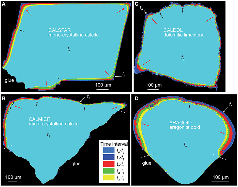
Figure 3. Cross-section of the superimposed volumes from t0 to t5, showing heterogeneous surface retreat with space and time. (A) CALSPAR, (B) CALMICR, (C) CALDOL, and (D) ARAGOID. The arrows point to large (red) or small (black) surface retreat in convex and concave areas, respectively.
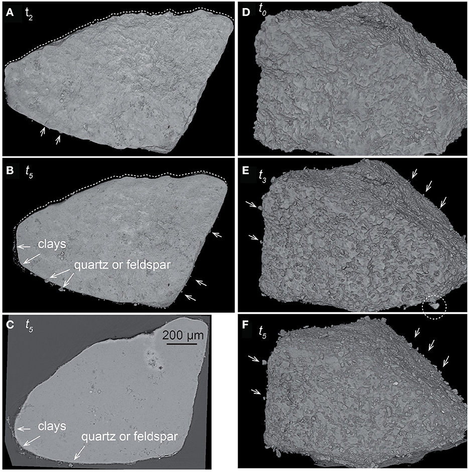
Figure 4. (A, B) XMT volume rendering and (C) cross-section of sample CALMICR at times t2 and t5. (D–F) Volume rendering of sample CALDOL at times t0, t3, and t5. The images show the evolution of the surface topography. Non-reactive silicate grains (i.e., quartz, feldspars, and clays) progressively appear (arrows) and detach (dotted circle) from the surface as dissolution progresses. The evolution of the surface roughness is also visible, with large-scale smoothing of the surface topography of CALMICR with time (dotted line), whereas the surface of CALDOL remains rough at all scales.
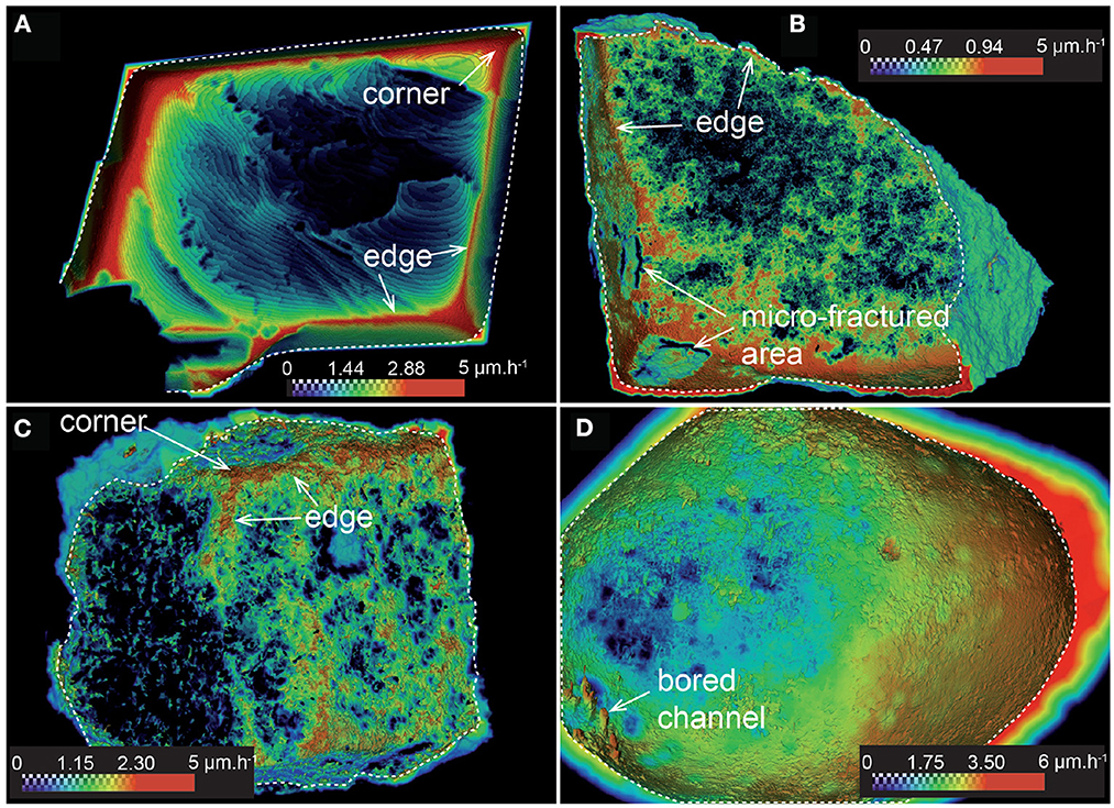
Figure 5. Local dissolution rate mapping at t4, showing the heterogeneous reaction rate distribution at the surface: (A) CALSPAR, (B) CALMICR, (C) CALDOL, and (D) ARAGOID. Only the area inside the dotted contours contains the rate data. The external part represents the distance map.
The rock fragments CALMICR and CALDOL show heterogeneous dissolution at their surface as well, and similarities regarding the topographical patterns of CALSPAR are noticed. The surface retreat is generally larger in areas of topographical highs (i.e., convex surface areas), like at the corners of CALSPAR, which are considered as the main contributors of reactivity. In contrast, surface retreat is smaller in the topographical lows (i.e., concave surface areas). For CALDOL, surprisingly, the dissolution rates of dolomite and calcite are within the same order of magnitude, although dolomite dissolution rate is generally considered to be one order of magnitude lower than calcite under acidic conditions (Morse and Arvidson, 2002). As a result, there is no increase in roughness at the scale of the calcite and dolomite patches in the rock fragment. Nevertheless, roughness develops at the sample surface (Figure 4) at two different scales: (i) at the micro-scale (μm), ghosts of carbonate crystals coated by clay particles are locally observed with SEM (Figure 1G), and (ii) at a larger scale, the presence of quartz and feldspar, whose dissolution rate is null at the timescale of the experiments, leads to the development of large-scale roughness (Figures 4D–F). The observation is similar for CALMICR at large scale, while the surface tends to become smoother at the micro-scale. However, in both samples, the progressive detachment of the non-reactive minerals from the surface contributes to the stabilization of the surface roughness through time.
Finally, for ARAGOID, the area of highest curvature shows the largest surface retreat. The surface of ARAGOID, which is initially very smooth (i.e., any crystal of aragonite can be distinguished with SEM) apart from areas close to the boring channels, becomes also rough, pointing to heterogeneous dissolution at the micro-scale (1–10 μm). The rate heterogeneity probably reflects the internal heterogeneity of the ooid, i.e., the size of the aragonite needle-like crystals (Figure 1H), their orientation, and the presence of micro-porosity, boring channels mostly localized below the grain surface, exogen materials forming the nucleus or organic coatings.
3.2. Dissolution rate and rate distribution
In the experiments, carbonate dissolution occurs under far-from-equilibrium conditions, with the saturation state Ω (Ω = IAP/Ksp, with IAP the ion activity product and Ksp the solubility product) with respect to calcite or aragonite remaining below 10−9. Tables 1–4 show the global rates derived from the volume difference calculation (, ) and from the surface retreat ('diss, and 'diss−norm). Figure 5 shows the distribution of the dissolution rates mapped at the surface of the samples. The differences between the global and local dissolution rates depend on the method used to calculate them. The values of and 'diss−norm differ by 40% in average. These differences are explained by the normalization of to the surface area of samples with different shapes and morphological evolution, like the surface roughness. As 'diss−norm derived from surface retreat provides a better estimate of the rate (see further discussion in Section 4.1), we will refer to this parameter for the description of the rates.
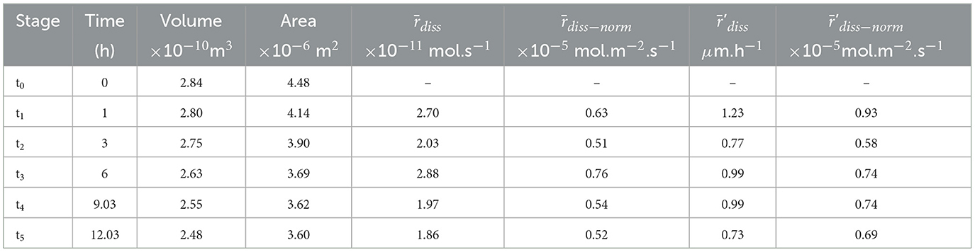
Table 2. Summary of the physical characteristics and reaction rates for sample CALMICR.

Table 3. Summary of the physical characteristics and reaction rates for sample CALDOL.
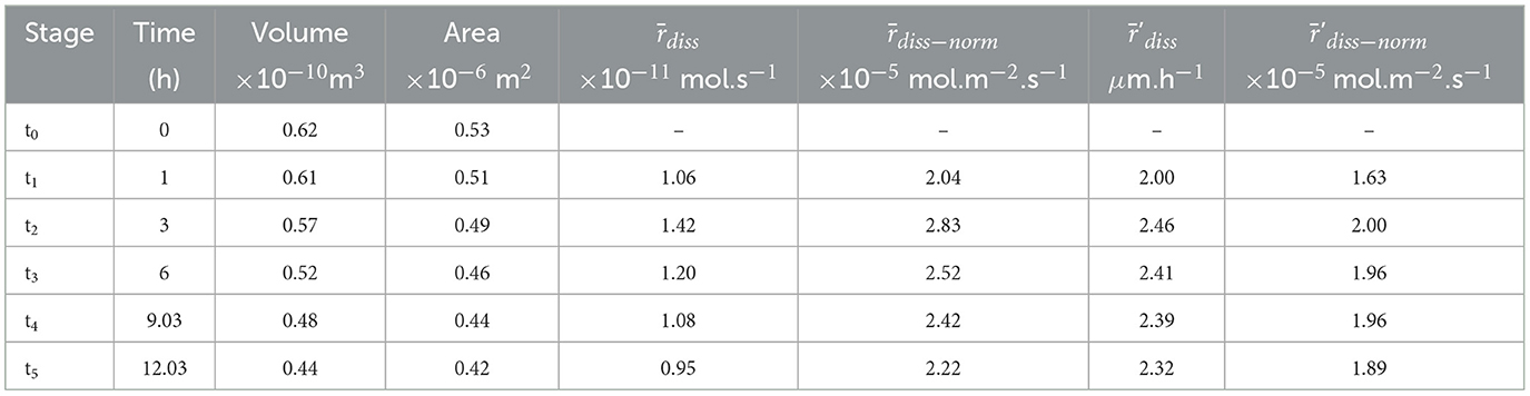
Table 4. Summary of the physical characteristics and reaction rates for sample ARAGOID.
Overall, the normalized rates are in the range 6–20 10−6 mol·m−2·s−1. Results show that the dissolution rate of aragonite (ARAGOID) is 1.4–2.0 times faster than calcite. Surprisingly, the dissolution rate of the calcite spar (CALSPAR) is 1.4 times faster in average than the micrite (CALMICR) or micro-sparite (CALDOL) grains. The temporal evolution of the reaction rates shows fluctuations with time (Tables 1–4). Overall, the dissolution rates of CALMICR, CALDOL, and ARAGOID decrease slightly with time, whereas the dissolution rate of CALSPAR is more constant.
The dissolution rate distributions are presented in Figures 6, 7. It is worth noting that the different points along the x-axis in the distributions are one pixel distant. Results first show that the histograms calculated for the intervals t0-t1 and t0-t2 are not sufficiently resolved, especially near zero. Each sample is characterized by a unique shape that accounts for the contribution of all the different geometry features to dissolution (Figure 6). The rate distribution is either asymmetric bell-type, right-skewed with a long tail (CALSPAR, CALMICR) or a short tail extending to the larger rates (CALDOL), or multi-modal (ARAGOID). The histograms are also truncated near zero for CALMICR and CALDOL, indicating a non-negligible fraction of null dissolution rates, in relation to the presence of the non-soluble silicate minerals. Temporal evolution of the histograms (Figure 7) shows different behaviors between the samples. For CALSPAR, the amount of low reactivity sites decreases, whereas the proportion of sites with dissolution rates in the range 1.4–2.8 μm·h−1 increases. For CALMICR, the amount of both low and high reactivity sites fluctuates. For CALDOL, the amount of high reactivity sites increases, as well as the proportion of sites whose reactivity is close to zero. For ARAGOID, the distributions vary significantly, with a change in intensity of the different modes as well as a shift of the histograms toward the lower rates.
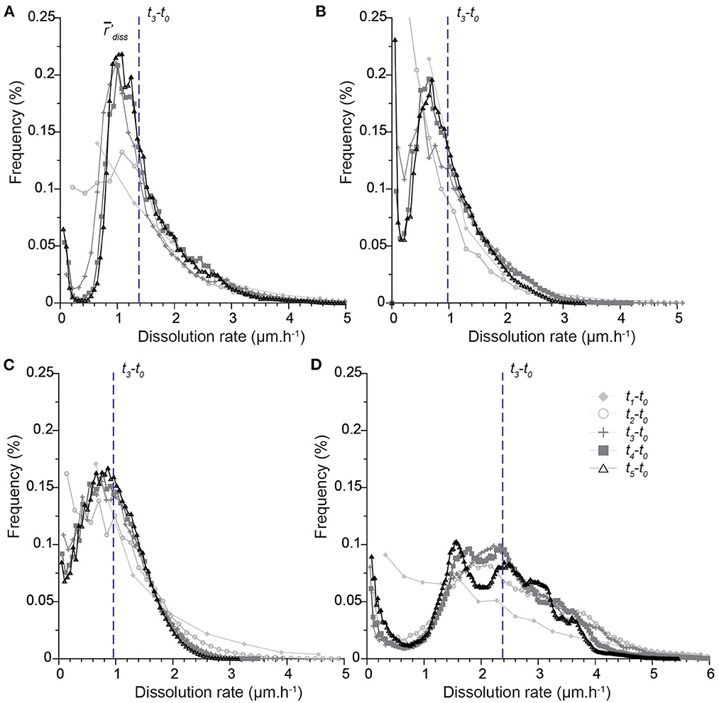
Figure 6. Distributions of dissolution rate r′diss in the time intervals ti-t0 (with 1≤i≤5) for the different samples: (A) CALSPAR [Adapted with permission from Noiriel et al. (2019). Copyright 2023 American Chemical Society], (B) CALMICR, (C) CALDOL*, and (D) ARAGOID*. All the histograms are normalized to a time of 6 h (corresponding to t3) and a pixel size of 0.65 μm, so that the surface areas below the curves are identical. The vertical line represents the average dissolution rate 'diss in the time interval t3-t0. *For the CALDOL and ARAGOID samples, a VOI containing only the first 800 top slices is considered in the calculation, so that the glued area does not alter the shape of the distribution near zero.
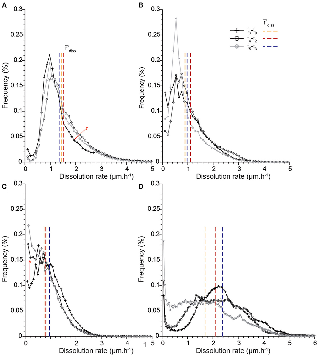
Figure 7. Temporal evolution of the distributions of dissolution rates in the time intervals t3-t0, t4-t2, and t5-t3: (A) CALSPAR, (B) CALMICR, (C) CALDOL, and (D) ARAGOID. The vertical lines represent the average dissolution rates 'diss in the different time intervals, and the red arrows show the major changes in the rate distributions through time.
3.3. Stochastic modeling
The geometry evolution of the Kossel crystal at the microscopic scale is directly related to the value of ϵ set in the kMC simulations (Supplementary Figures 1–3). A low value of ϵ leads to a high probability of detachment of face elements, , compared to edges and corner elements. In contrast, a high value of ϵ leads to a high probability of detachment of corner elements, , thus enhancing dissolution at corners and edges of the crystal compared to their faces. High values of (1) clearly result in faceting along the {111} planes (Supplementary Figure 1), whereas favors delamination of the {100}, {010}, and {001} faces with a moderate effect at the crystal edges and corners (Supplementary Figure 3). Kinetic Monte Carlo modeling shows that the corner elements become progressively the main contributors to dissolution, and the normalized sets of probabilities converge on the long term, i.e., after about 10% of the Kossel crystal is dissolved. There is a link between the bound-breaking activation energy Eb (through the value of ϵ) and the converged set of probabilities obtained. The results obtained from kMC simulations are applicable in the stochastic model at larger scale, where large similarities are noticed between the geometry of the nanosized crystal and the geometry of the macroscopic crystal (Supplementary Figures 1–3). Overall, the main features developing at the crystal corners, edges, and faces from the macroscopic stochastic model are conserved.
Similarly to kMC, the set of probabilities chosen in the macroscopic stochastic model also influences the retreat at the macroscopic scale (i.e., crystal geometry). In particular, the surface retreat at the crystal corners, edges and faces, as well as the retreat magnitude at topographical lows and highs, depend on the set {Pc, Pe, Pf}. The converged set derived from ϵ = 0.03 in kMC simulations is appropriate to describe the dissolution of the CALSPAR crystal, when balancing the contribution of the faces and of the corners to the global retreat (Figure 8). Output volumes are generated after the iterations (it.) 20, 60, 137, 209, and 237, which correspond to jV1 to jV5, respectively.
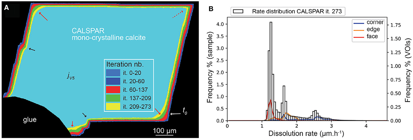
Figure 8. (A) Evolution of the CALSPAR geometry (displayed as a cross-section) from stochastic modeling using the set of probabilities obtained with ϵ = 0.03. (B) Corresponding dissolution rate distribution at jV5, corresponding to iteration 273, including the three VOIs at crystal edge, face, and corner. The arrows point to high (red) or low (black) surface retreat in convex and concave areas, respectively, similarly to the experimental observations. The red dotted arrow point to the VOIc which does not dissolve as fast as it should due to the presence of a flat surface area in the XMT volume of interest.
The geometry evolution of the CALSPAR calcite crystal is presented in Figure 8, together with the dissolution rate distribution at iteration 237 for the crystal and its three volumes of interest, VOIc, VOIe, and VOIf. The dissolution rates are presented in Table 5. The rate distribution of all the outputs are presented in Supplementary Figures 5–8. At the end of the simulation, the dissolution rate varies between 1 and 4 μm·h−1 with three peak maxima at about 1.4, 1.6, and 2.4 μm·h−1. The mean rate is equal to 1.59 μm·h−1. The VOIf, VOIe, and VOIc dissolve at 1.26, 1.68, and 2.26 μm·h−1, respectively. However, contrary to the experiment, the distributions of VOIc and VOIe are bimodal. This results are explained by the fact that these VOIs exhibit both a flat surface portion and a very stepped surface portion, resulting in two very different rates of dissolution. The dissolution rates of the VOIf and VOIc are also slightly higher and lower than in the experiment, respectively.
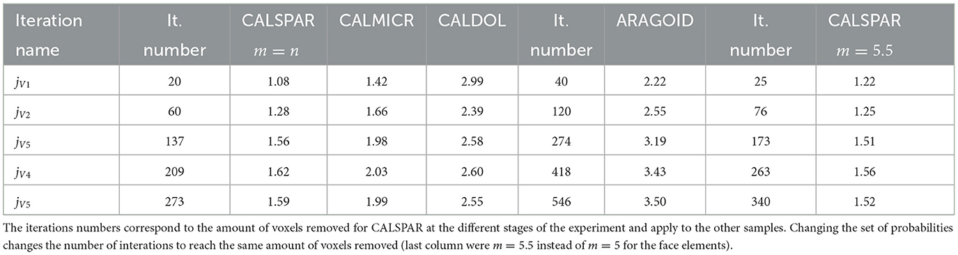
Table 5. Average dissolution rates (mol·s−1) derived from the macroscopic stochastic model.
It is possible to reduce the contribution of the crystal faces to dissolution and increase that of the corners by increasing m for the face elements in Equation (12), thus decreasing Pf. Taking m = 5.5 to describe the reactivity of the face elements leads to the probability set: . For the same amount of voxels removed, the number of iterations jV1 to jV5 increases compared to the case where m = n. In addition, the average dissolution rate is a bit lower, translating into a slight decrease in the global reactivity of the crystal (Table 5). This is the consequence of decreasing the reactivity of the faces, although the reactivity at corners and edges is increased (Figure 9). The three peak maxima are at 0.9, 1.7, and 3.1 μm·h−1. The VOIf, VOIe and VOIc dissolve at 0.91, 1.98, and 3.18 μm·h−1, respectively, close to the values of 0.87, 1.52, and 3.14 μm·h−1 determined experimentally for these VOIs in Noiriel et al. (2019).
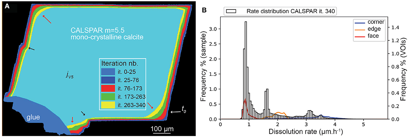
Figure 9. (A) Evolution of the CALSPAR geometry (displayed as a cross-section) from stochastic modeling using the set of probabilities obtained with ϵ = 0.03 and m = 5.5 in Equation (12) at the five iterations jV1=it. 25 to jV5=it. 340. (B) Corresponding dissolution rate distribution at iteration 340, including the three VOIs at crystal edge, face, and corner. The arrows point to high (red) or low (black) surface retreat in convex and concave areas, respectively, similarly to the experimental observations.
Application of the set of probabilities to the three other samples gives the following results. Globally, all the samples dissolve faster than CALSPAR (Table 5), in relationship with a higher amount of corner elements initially present at the fluid-mineral interface for these geometries. Similarly to CALSPAR, dissolution is higher in convex areas compared to flat or concave areas (Figure 10, left). Figure 10A shows the dissolution rate of sample CALMICR. The highest peak of dissolution rate is found at about 1.6 μm·h−1. The distribution is skewed right with a long tail, and translates directly the behavior of the convex and concave areas, as underlined by the VOIconvex and VOIconcave in Figure 10A (left).
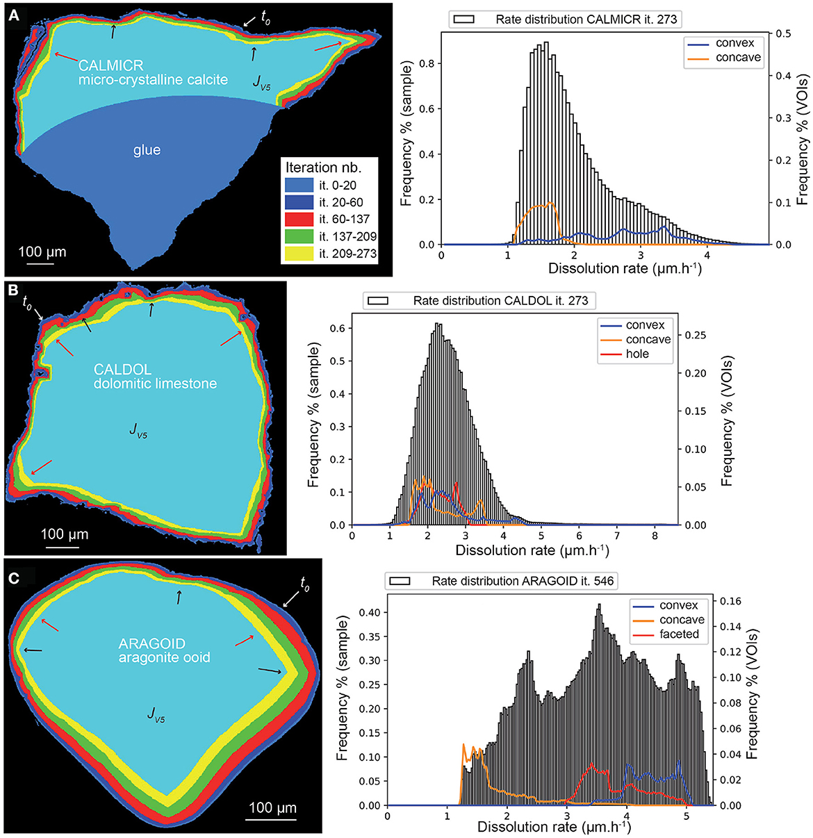
Figure 10. Evolution (left) of the geometry of (A) CALMICR, (B) CALDOL, and (C) ARAGOID samples (displayed as superimposed cross-sections) from stochastic modeling at the five iterations jV1= it. 20 (40 for ARAGOID) jV5= it. 273 (546 for ARAGOID) and (right) corresponding dissolution rate distributions at iteration jV5. The arrows point to high (red) or low (black) surface retreat in convex and concave areas similarly to the experimental observations.
In contrast, the dissolution rate distribution of CALDOL is nearly Gaussian (Figure 10B), similarly to the experimental results, and most of the dissolution occurs at rates in the range 1–5 μm·h−1, with the highest peak at 2.3 μm·h−1. However, contrary to the experiment, near-zero rates do not exist as the non-soluble minerals are not accounted for in the simulations. In addition, a few data points reach a high dissolution rate (in between 5 and 8 μm·h−1), in relationship with the presence of micro-fractures and deep connected pores below the surface that alter the distance map. All the VOIs dissolve in average at the same rate (2.3 μm·h−1), something explained by the rapid evolution of the surface roughness for this sample, meaning that it was difficult to define proper convex and concave surface areas over time. The VOIpore, which represents a connected pore below the surface (see Figure 10B), does not pose any problem here in the retreat determination.
Finally, the dissolution rate for the aragonite sample ARAGOID (Figure 10C) is higher than the other three samples, with several peaks in the rate distribution. The distribution of rates is also more spread out. It is worth noting that the initial rounded geometry of the ooid also evolves toward a more faceted geometry (Figure 11).
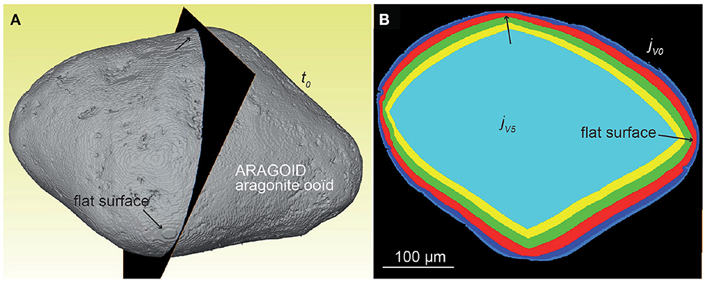
Figure 11. Evolution of the geometry of sample ARAGOID (displayed as superimposed cross-sections) depicting faceting during stochastic modeling. (A) Geometry of the sample at time t0; the vertical slice indicates the position of the cross-sections shown in (B).
4. Discussion
4.1. Application of X-ray micro-tomography for tracking mineral and rock reactivity
Like techniques measuring the surface retreat, XMT offers the possibility to determine the retreat at the fluid-mineral interface, with an estimated error of ±1 pixel (see Noiriel et al., 2020 for a comparison with vertical scanning interferometry measurements). Between 2.1 and 5.6 million data points for retreat were considered initially at the surface of the different samples. The technique has the advantage over bulk experiments on mineral powders of bypassing the process of normalization to the surface area (Noiriel and Daval, 2017), which depends on either the geometric surface area calculated from the crystal size or the Brunauer-Emmett-Teller (BET) surface area determined from gas adsorption (Brunauer et al., 1938). The rates derived from surface retreat ('diss−norm) and the rates derived from the volume difference calculation and normalized to the geometric surface area () do not match in the experiments (Tables 1–3). The specific surface area of the unreacted samples determined at the scale of the XMT imaging technique are equal to 46.8, 58.3, 67.0, and 31.4 cm2·g−1 for CALSPAR, CALMICR, CALDOL, and ARAGOID, respectively, compared to the BET surface area of 120 cm2·g−1 of similar calcite crystals (Noiriel et al., 2012, 2019), and reported values of 85.6 and 56.4 cm2·g−1 for aragonite oolites (Busenberg and Plummer, 1986). Normalization to the geometric surface area obtained from XMT compared to normalization to the BET surface area provides rates closer to the rate derived from surface retreat. The maximum difference is 55% when comparing diss−norm to 'diss−norm, and discrepancies can be reduced after correction from the covering effect of the glue. Normalization to the BET surface area would have increased the discrepancy between diss−norm and 'diss−norm. The two-to-three times difference in surface area may be explained by a surface roughness of the grains that is not visible at the resolution of XMT imaging and by the internal micro-porosity.
Application of the distance map is an indirect method to determine the surface retreat. The procedure has the advantage to provide a rapid determination of the retreat at the whole sample surface, even if limitations exist, like the estimation of the distance between highly curved interfaces (Sethian, 1999) in relation to the choice of a reference volume from which the distance map is calculated (Noiriel and Soulaine, 2021). The choice for a reference volume, e.g., the initial or the final geometry, does indeed influence the highest values of retreat (e.g., see Noiriel and Soulaine, 2021 for a comparison), especially for samples depicting sharp surface curvatures. Micro-fractures or internal non-connected porosity could also introduce some bias in the estimation of the surface retreat, even if the phenomenon is limited to a very low portion of the fluid-mineral surface area, and that the internal, non-connected porosity was filled following the segmentation of the images to minimize such a bias.
4.2. Stochastic dissolution of carbonate minerals and limestone
Kinetic Monte Carlo modeling is not possible on mm-scale samples due to the large size domain and iterations required from atomistic considerations. Although techniques are currently developed to deal with large-size geometries, like the use of Voronoï diagrams coupled to distance mapping (Rohlfs et al., 2018), the loss of atomic-scale mechanistic description is currently a limitation to obtain models that are generalizable and applicable to a wide range of systems and physico-chemical conditions. The stochastic macroscopic model developed in this study has the credit to relate the mechanistic description used in the kMC framework to a larger scale. Indeed, the kMC simulations on small Kossel crystals provide a set of converged probabilities that is applicable to describe the geometry evolution of the samples at the macroscopic scale. For a given value of ϵ, observations that: i) the kMC set of probabilities converges and ii) the geometry evolution of the nanosized crystal in kMC resembles that of the large scale crystal obtained from the macroscopic stochastic model have permitted to derive a set of probabilities which can be applied to mimic dissolution of large-scale samples. In addition, kMC simulations show that there is a link between the bound-breaking activation energy Eb (through the value of ϵ) and the converged set of probabilities obtained. Looking at the contribution of the different types of sites to the crystal dissolution rate obtained by Ackerer et al. (2021) for a Kossel crystal, it would translate in our experiments to a value of Eb in the range 6–9 kJ·mol−1 for calcite dissolution at pH 4.0, a value quite consistent with the values of the macroscopic activation energy Ea of 8.4–19 kJ·mol−1 reported in the literature for calcite under acidic conditions (Alkattan et al., 1998; Morse and Arvidson, 2002; Palandri and Kharaka, 2004), considering that Ea≃3Eb when the corner elements dominate the dissolution process (Ackerer et al., 2021), i.e., close to 1.
The value of ϵ = 0.03 used in the macroscopic stochastic model is only constrained by the geometry evolution of the calcite spar crystal obtained with XMT regarding the dissolution rate at crystal faces, edges, and corners. This value is far from the value of ϵ~1.4 10−3 used by Carrasco and Aarão Reis (2021) in kMC simulations to describe dissolution of nanosized crystals whose dissolution rate is similar to that of our experiments. The reason is that nanosized crystals dissolve much faster than macroscopic crystals (Briese et al., 2017), so that the activation energy should be smaller than for macroscopic crystals (Carrasco and Aarão Reis, 2021). As a consequence, a nanosized crystal and a mm-size crystal both dissolving at the same rate will result in a value of ϵ higher for the larger crystal. We argue that a kMC simulation that could be run on a mm-size crystal (i.e., a domain of about 2.5 106×2.5 106×2.5 106 elements) with ϵ≃1.4 10−3 would give a set of probabilities close to the one obtained with ϵ = 0.03 with the Kossel crystal of 100 × 100 × 100 elements in size, i.e., . In addition, it should be possible to find the best set of probabilities {Pc, Pe, Pf} by running a series of simulations with different combinations and finding the best match with the experimental results by optimizing a metrics (for instance the histogram distribution of the geometrical shape). Although our approach of upscaling is very different from Carrasco and Aarão Reis (2021) and requires experimental data to be constrained, it seems promising to evaluate the role of the crystal (or grain) geometry, which is now viewed as in intrinsic cause of variability in the dissolution rate distribution of samples (Pollet-Villard et al., 2016; Noiriel and Daval, 2017), in relation to the density of the different types of sites (kinks, steps, terraces) at their surface.
Stochastic modeling at the crystal or rock fragment scale reproduces the larger surface retreat at the crystal corners, edges, and topographical highs (i.e., convex interfaces), compared to flat interfaces or topographical lows (i.e., concave surfaces), as observed in the experiments. The assumption behind stochastic modeling is that the dissolution rate is related to bond-breaking probabilities, following Equation (1) In other words, surface reaction-controlled conditions are assumed, whereas transport of reactants and products at the fluid-mineral interface are not considered in the global reaction. Interestingly, the results show that a surface reaction-controlled model can lead to smoothing of the rough surfaces, including crystal edges, and corners, similarly to what is routinely observed in reactive-transport modeling in transport-controlled conditions. Indeed, smoothing of the rough surfaces during reactive-transport modeling is unlikely to happen in surface reaction-controlled conditions where a simple translation of the fluid-mineral interface is expected, as observed for instance by Yuan et al. (2019) or Noiriel and Soulaine (2021). Although dissolution of carbonates at pH = 4 is admitted to be at least partly diffusion-limited (Morse and Arvidson, 2002), with an effect on crystal smoothing, diffusion-limited conditions are not a prerequisite to decrease surface roughness during dissolution.
The role of surface roughness is evident at the small scale, like shown in the kMC simulations of de Assis and Aarao Reis (2018). At larger scale, evolution of surface roughness is less evident as the surface will be composed of both convex and concave surfaces areas and averaging over these two types of features will occur. Apart from the calcite spar, the shape of the dissolution rate distributions are in reasonably good agreement with the distributions derived from the experiments. This observation tends to demonstrate that the geometry of a grain has a huge influence on its reactivity, an effect important to account for in laboratory studies on mineral powders, where grinding and sieving of large crystals or rock samples is common. This effect is also important regarding studies that focus only on retreat determination of well-cleaved flat surfaces. It is also important to account for this effect in relationship that relate, for instance, porosity to permeability in reactive transport models, as evolution of these parameters could be linked to the rock fabric (Noiriel et al., 2019).
The dissolution rate distribution of the calcite spar, however, is not quite similar to the distribution obtained experimentally, with the three modes for crystal corners, edges and faces more pronounced in the simulations than in the experiments. It is worth noting that decreasing the contribution of the faces to dissolution by taking m = 5.5 for the face elements like Carrasco and Aarão Reis (2021) reproduces better both the average rate (Tables 1, 5) and the range of dissolution rates (Figures 6A, 9B). The deviation from the terrace-ledge-kink model (where n = 3, 4, 5 instead of m = 3, 4, 5.5 here) better fits with the experimental measurements at the faces of calcite in far-from-equilibrium conditions (Ruiz-Agudo et al., 2009) where the density of shallow pits (i.e., etch pits which are not associated to surface defects but form at the flat surface) suggest a lower detachment rate than expected by the theory (Carrasco and Aarão Reis, 2021). This interpretation is also supported by ab initio predictions that show that the activation energy at terrace site (Raiteri et al., 2010) is far higher than the one estimated in the terrace-ledge-kink model. In addition, the fact that the three peaks for VOIs corners, edges and face are well-separated in the simulation compared to the experiment tends to demonstrate that either the macroscopic stochastic model lacks of randomness (a randomness that could be introduced by not removing the totality of the elements in a class at each iteration—although it would result in a loss of mechanistic description regarding theoretical considerations), or that the choice to take elements of size of the XMT voxel size regarding the geometry of the crystal (i.e., a rhombohedron with well-cleaved faces) creates upscaling issues.
The rates obtained for the other three samples (CALMICR, CALDOL, and ARAGOID), while keeping the same iteration numbers for the outputs, are over-evaluated, translating a higher fraction of corner elements initially at the surface of these geometries compared to CALSPAR, which exhibits quite well-cleaved faces. As a consequence, the three samples dissolve faster in the simulations than in the experiments. It is worth noting that the stochastic model did not account for the intrinsic reactivity of the samples. The fact that the micritic or the dolomitic limestone rock fragments dissolve slower in the experiments than the calcite spar is unusual given the size of the individual grains forming the rock fragments and the presence of dolomite, in comparison with the calcite spar crystal. This intrinsic difference in reactivity is probably explained by the presence of a small fraction of clays (< 1%) that could limit the diffusion of reactants toward the fluid-mineral interface. To account for this effect, a different parameterization of the stochastic model could be performed in a future study.
Finally, it is worth pointing at the discretization of sample geometries from XMT imaging and for stochastic modeling of dissolution to explain some discrepancies between the experimental and the numerical results. As shown by Carrasco and Aarão Reis (2021), dissolution of a Kossel crystal and of the equivalent rotated cube exhibiting many surface edges elements results both in different rate distributions and dissolution patterns. The discretization of the sample does influence the surface retreat in the simulations. For instance, the sample CALSPAR, as a rhombohedron-shape crystal, has the largest faces approximately parallel to one of the three Cartesian planes, while the other faces intersect the other Cartesian planes. As a consequence, the faces parallel to a Cartesian plane have a larger number of face elements compared to the faces intersecting the Cartesian planes, which result in the latter case in a higher surface retreat (visible in Figures 8, 9 on the left and right sides of the crystal). Performing simulations in the lattice system of the crystal could help to eliminate this effect, although this supposes also a transformation of the unit cell of XMT (i.e., the cubic voxel) into the new lattice system, with a possible decrease of spatial resolution due to the subsequent interpolation. At smaller scale, the presence of flat areas could also determine the long term evolution of the geometries. For instance, a flat area in the VOIc of CALSPAR explains why the retreat at corner of the calcite spar crystal is bimodal (Figure 8B). More importantly, the small flat areas in ARAGOID, which would result in any discretization of a sphere in Cartesian coordinates, is responsible for the faceting development of the presumably rounded aragonite ooid in the simulations (Figures 10C, 11). Indeed, approximation of a sphere in a Cartesian coordinate systems leads to six small flat surfaces with orientation {100}, {010} {001}. The highest number of face elements in these areas leads to a lower surface retreat and consequent development of {111} facets, as already observed by Carrasco and Aarão Reis (2021). Faceting at low ϵ values appears as one of the major upscaling issue of the macroscopic stochastic model. Indeed, faceting translates into a decrease of the surface retreat heterogeneity over the {111} planes in between microscopic and macroscopic scale (Supplementary Figure 1).
The last limitation of stochastic modeling is the presence of impurities or secondary minerals in the rock fragments, i.e., quartz, clays, or dolomite, which are not accounted for in the model, in which the surface roughness tends to smooth out with time, whereas the micritic and dolomitic limestone rocks show clearly an increase in surface roughness at the mineral scale during the experiments. Dissolution of rocks will be anyway more complex to assess compared to single crystals, as rocks also contain accessory minerals that can influence the global dissolution process. Reactive minerals are also either randomly oriented or exhibit a fabric, which will also play a role on the dissolution rate variability at the surface (Pedrosa et al., 2021).
5. Conclusions
We have presented an experimental and stochastic modeling study exploring the dissolution rates of four carbonate samples under acidic (pH 4), far-from-equilibrium conditions, deriving rates from XMT imaging with a sub-micron resolution. The experimental results reveal that the dissolution rate variability at the fluid-mineral surface depends on the carbonate type (calcite vs. aragonite, sparite vs. micrite, single crystal vs. rock fragment or grain), and on the sample geometry. A main common geometrical feature is higher dissolution rates at crystal corners and edges and at rock or grain convex areas (topographical highs), compared to flat surface or topographical lows. High dissolution rates correspond to high energy sites, at which reactivity is enhanced. This process can be accounted for in stochastic modeling constrained by the geometries obtained from X-ray micro-tomography after segmentation of the 3D images. Stochastic modeling at the sample scale was parameterized from kinetic Monte Carlo simulations on a Kossel crystal at the microscopic scale, from which a normalized and converged set of probabilities was derived in steady-state regime of dissolution. Although fine details at the surface, anisotropy at reactive sites, and intrinsic variability between carbonate samples cannot be reproduced by the model, overall it is possible to reproduce at the mm-scale the dissolution mechanisms at play at the microscopic scale. Thanks to the experimental approach combining dissolution experiments on single crystals or grains and 4D XMT, our modeling approach can easily bypass the limitations of kinetic Monte Carlo modeling in handling large-size systems.
The variability in reactivity is expected, however, to be different in more neutral and close-to- equilibrium conditions. Some extensions of this work concern (i) geochemical conditions and saturation states closer to those encountered in most natural systems, (ii) consideration of the individual behavior of minerals in polymineralic rocks, like in the dolomitic limestone, or in the micritic limestone where the presence of clay or quartz minerals may affect the rate distribution, and (iii) the effect of anisotropy in dissolution of calcite along the and directions, which should be at play to explain the acute vs obtuse step retreat difference commonly observed in etch pits (Jordan and Rammensee, 1998; De Giudici, 2002), cleavages (Noiriel et al., 2020), and at the crystal edges.
Data availability statement
The raw data supporting the conclusions of this article will be made available by the authors, without undue reservation.
Author contributions
MG developed the stochastic models for dissolution and performed numerical simulations. CN conceived and supervised the project, carried out the experiments, processed the imaging data, performed numerical simulations, and analyzed the results. CN and MG wrote the manuscript. All authors discussed the stochastic models, provided critical feedback, and contributed to the final version of the manuscript.
Acknowledgments
The Institut Carnot ISIFOR funded this work under project MICROTRANSPHASIQUE 451216. We acknowledge the Paul Scherrer Institute for provision of synchrotron radiation beamtime at Swiss Light Source, TOMCAT beamline X02DA. Local contacts David Haberthür and Iwan Jerjen are acknowledged for their assistance with image acquisition.
Conflict of interest
The authors declare that the research was conducted in the absence of any commercial or financial relationships that could be construed as a potential conflict of interest.
Publisher's note
All claims expressed in this article are solely those of the authors and do not necessarily represent those of their affiliated organizations, or those of the publisher, the editors and the reviewers. Any product that may be evaluated in this article, or claim that may be made by its manufacturer, is not guaranteed or endorsed by the publisher.
Supplementary material
The Supplementary Material for this article can be found online at: https://www.frontiersin.org/articles/10.3389/frwa.2023.1185608/full#supplementary-material
References
Ackerer, P., Bouissonnié, A., di Chiara Roupert, R., and Daval, D. (2021). Estimating the activation energy of bond hydrolysis by time-resolved weighing of dissolving crystals. NPJ Mater. Degrad. 5:48. doi: 10.1038/s41529-021-00196-z
Akmal Butt, M., and Maragos, P. (1998). Optimum design of chamfer distance transforms. IEEE Trans. Image Process. 7, 1477–1484. doi: 10.1109/83.718487
Alkattan, M., Oelkers, E. H., Dandurand, J.-L., and Schott, J. (1998). An experimental study of calcite and limestone dissolution rates as a function of ph from -1 to 3 and temperature from 25 to 80°C. Chem. Geol. 151, 199–214. doi: 10.1016/S0009-2541(98)00080-1
Andersen, M., Panosetti, C., and Reuter, K. (2019). A practical guide to surface kinetic Monte Carlo simulations. Front. Chem. 7:202. doi: 10.3389/fchem.2019.00202
Arvidson, R. S., Beig, M. S., and Lüttge, A. (2004). Single-crystal plagioclase feldspar dissolution rates measured by vertical scanning interferometry. Am. Mineral. 89, 51–56. doi: 10.2138/am-2004-0107
Bandstra, J. Z., and Brantley, S. L. (2008). Surface evolution of dissolving minerals investigated with a kinetic Ising model. Geochim. Cosmochim. Acta 72, 2587–2600. doi: 10.1016/j.gca.2008.02.023
Brand, A. S., Feng, P., and Bullard, J. W. (2017). Calcite dissolution rate spectra measured by in situ digital holographic microscopy. Geochim. Cosmochim. Acta 213, 317–329. doi: 10.1016/j.gca.2017.07.001
Briese, L., Arvidson, R. S., and Luttge, A. (2017). The effect of crystal size variation on the rate of dissolution: a kinetic Monte Carlo study. Geochim. Cosmochim. Acta 212, 167–175. doi: 10.1016/j.gca.2017.06.010
Brunauer, S., Emmet, P. H., and Teller, E. A. (1938). Adsorption of gases in multimolecular layers. J. Am. Chem. Soc. 60, 309–319. doi: 10.1021/ja01269a023
Busenberg, E., and Plummer, L. N. (1986). “A comparative study of the dissolution and precipitation kinetics of calcite and aragonite,” in Studies in Diagenesis, U. S. Geological Survey Bulletin, ed F. A. Mumton (Washington, DC: U.S. Geological Survey), 139–168.
Carrasco, I. S. S., and Aarão Reis, F. D. A. (2021). Modeling the kinetics of calcite dissolution in neutral and alkaline solutions. Geochim. Cosmochim. Acta 292, 271–284. doi: 10.1016/j.gca.2020.09.031
Colombani, J. (2016). The alkaline dissolution rate of calcite. J. Phys. Chem. Lett. 7, 2376–2380. doi: 10.1021/acs.jpclett.6b01055
de Assis, T. A., and Aarao Reis, F. D. A. (2018). Dissolution of minerals with rough surfaces. Geochim. Cosmochim. Acta 228, 27–41. doi: 10.1016/j.gca.2018.02.026
De Giudici, G. (2002). Surface control vs. diffusion control during calcite dissolution: dependence of step-edge velocity upon solution ph. Am. Mineral. 87, 1279–1285. doi: 10.2138/am-2002-1002
de Leeuw, N. H., Parker, S. C., and Harding, J. H. (1999). Molecular dynamics simulation of crystal dissolution from calcite steps. Phys. Rev. B 60, 13792–13799. doi: 10.1103/PhysRevB.60.13792
Emmanuel, S. (2014). Mechanisms influencing micron and nanometer-scale reaction rate patterns during dolostone dissolution. Chem. Geol. 363, 262–269. doi: 10.1016/j.chemgeo.2013.11.002
Eyring, H. (1935). The activated complex and the absolute rate of chemical reactions. Chem. Rev. 17, 65–82. doi: 10.1021/cr60056a006
Fenter, P., Geissbühler, P., DiMasi, E., Strajer, G., Sorenssen, L. B., and Sturchio, N. C. (2000). Surface speciation of calcite observed in situ by high-resolution X-ray reflectivity. Geochim. Cosmochim. Acta 64, 1221–1228. doi: 10.1016/S0016-7037(99)00403-2
Fischer, C., Kurganskaya, I., and Luttge, A. (2018). Inherited control of crystal surface reactivity. Appl. Geochem. 91, 140–148. doi: 10.1016/j.apgeochem.2018.02.003
Fischer, C., and Luttge, A. (2007). Converged surface roughness parameters—A new tool to quantify rock surface morphology and reactivity alteration. Am. J. Sci. 307, 955–973. doi: 10.2475/07.2007.01
Gilmer, G. H. (1977). Computer simulation of crystal growth. J. Cryst. Growth 42, 3–10. doi: 10.1016/0022-0248(77)90170-1
Gilmer, G. H. (1980). Transients in the rate of crystal growth. J. Cryst. Growth 49, 465–474. doi: 10.1016/0022-0248(80)90121-9
Godinho, J. R. A., Piazolo, S., and Evins, L. Z. (2012). Effect of surface orientation on dissolution rates and topography of CaF2. Geochim. Cosmochim. Acta 86, 392–403. doi: 10.1016/j.gca.2012.02.032
Hillner, P. E., Gratz, A. J., Manne, S., and Hasma, P. K. (1992). Atomic-scale imaging of calcite growth and dissolution in real time. Geology 20, 359–362. doi: 10.1130/0091-7613(1992)020<0359:ASIOCG>2.3.CO;2
Jansen, A. (2012). An Introduction to Kinetic Monte Carlo Simulations of Surface Reactions. Berlin; Heidelberg: Springer. doi: 10.1007/978-3-642-29488-4
Jordan, G., and Rammensee, W. (1998). Dissolution rates of calcite (104) obtained by scanning force microscopy: microtopography-based dissolution kinetics on surfaces with anisotropic step velocities. Geochim. Cosmochim. Acta 62, 941–947. doi: 10.1016/S0016-7037(98)00030-1
Kossel, W. (1927). Zur theorie des kristallwachstums. Nachrichten von der Gesellschaft der Wissenschaften zu Göttingen. Math. Phys. Klasse 1927, 135–143.
Kurganskaya, I., and Churakov, S. V. (2018). Carbonate dissolution mechanisms in the presence of electrolytes revealed by grand canonical and kinetic Monte Carlo modeling. J. Phys. Chem. C 122, 29285–29297. doi: 10.1021/acs.jpcc.8b08986
Kurganskaya, I., and Luttge, A. (2016). Kinetic Monte Carlo approach to study carbonate dissolution. J. Phys. Chem. C 120, 6482–6492. doi: 10.1021/acs.jpcc.5b10995
Kurganskaya, I., and Rohlfs, R. D. (2020). Atomistic to meso-scale modeling of mineral dissolution: methods, challenges and prospects. Am. J. Sci. 320, 1–26. doi: 10.2475/01.2020.02
Laanait, N., Callagon, E. B. R., Zhang, Z., Sturchio, N. C., Lee, S. S., and Fenter, P. (2015). X-ray-driven reaction front dynamics at calcite-water interfaces. Science 349, 1330–1334. doi: 10.1126/science.aab3272
Lardge, J. S., Duffy, D., Gillan, M., and Watkins, M. (2010). Ab initio simulations of the interaction between water and defects on the calcite 104 surface. J. Phys. Chem. C 114, 2664–2668. doi: 10.1021/jp909593p
Lasaga, A. C., and Blum, A. E. (1986). Surface chemistry, etch pits and mineral-water reactions. Geochim. Cosmochim. Acta 50, 2363–2379. doi: 10.1016/0016-7037(86)90088-8
Lasaga, A. C., and Luttge, A. (2001). Variation of crystal dissolution rate based on a dissolution stepwave model. Science 291, 2400–2404. doi: 10.1126/science.1058173
Liang, Y., Baer, D. R., McCoy, J. M., Amonette, J. M., and LaFemina, J. P. (1996). Dissolution kinetics at the calcite-water interface. Geochim. Cosmochim. Acta 60, 4883–4887. doi: 10.1016/S0016-7037(96)00337-7
Luttge, A., Arvidson, R. S., Fischer, C., and Kurganskaya, I. (2019). Kinetic concepts for quantitative prediction of fluid-solid interactions. Chem. Geol. 504, 216–235. doi: 10.1016/j.chemgeo.2018.11.016
Marone, F., and Stampanoni, M. (2012). Regridding reconstruction algorithm for real-time tomographic imaging. J. Synchrot. Radiat. 19, 1029–1037. doi: 10.1107/S0909049512032864
McCoy, J., and LaFemina, J. P. (1997). Kinetic Monte Carlo investigation of pit formation at the CaCO3 (104) surface-water interface. Surface Sci. 373, 288–299. doi: 10.1016/S0039-6028(96)01156-9
Meakin, P., and Rosso, K. M. (2008). Simple kinetic Monte Carlo models for dissolution pitting induced by crystal defects. J. Chem. Phys. 129:204106. doi: 10.1063/1.3021478
Morse, J. W., and Arvidson, R. S. (2002). The dissolution kinetics of major sedimentary carbonate minerals. Earth-Sci. Rev. 58, 51–84. doi: 10.1016/S0012-8252(01)00083-6
Noiriel, C., and Daval, D. (2017). Pore-scale geochemical reactivity associated with CO2 storage: new frontiers at the fluid-solid interface. Acc. Chem. Res. 50, 759–768. doi: 10.1021/acs.accounts.7b00019
Noiriel, C., and Deng, H. (2018). Evolution of planar fractures in limestone: the role of flow rate, mineral heterogeneity and local transport processes. Chem. Geol. 497, 100–114. doi: 10.1016/j.chemgeo.2018.08.026
Noiriel, C., Oursin, M., and Daval, D. (2020). Examination of crystal dissolution in 3D: a way to reconcile dissolution rates in the laboratory? Geochim. Cosmochim. Acta 273, 1–25. doi: 10.1016/j.gca.2020.01.003
Noiriel, C., Oursin, M., Saldi, G. D., and Haberthür, D. (2019). Direct determination of dissolution rates at crystal surface using 3D X-ray micro-tomography. Earth Space Chem. 3, 101–108. doi: 10.1021/acsearthspacechem.8b00143
Noiriel, C., and Renard, F. (2022). 4D X-ray micro-tomography imaging of dynamic processes in geosciences. Compt. Rendus Geosci. 354, 255–280. doi: 10.5802/crgeos.137
Noiriel, C., and Soulaine, C. (2021). Pore-scale imaging and modelling of reactive flow in evolving porous media: tracking the dynamics of the fluid-rock interface. Transp. Porous Media 140, 181–213. doi: 10.1007/s11242-021-01613-2
Noiriel, C., Steefel, C. I., Yang, L., and Ajo-Franklin, J. (2012). Upscaling calcium carbonate precipitation rates from pore to continuum scale. Chem. Geol. 318–319, 60–74. doi: 10.1016/j.chemgeo.2012.05.014
Palandri, J. L., and Kharaka, Y. K. (2004). A Compilation of Rate Parameters of Water-Mineral Interaction Kinetics for Application to Geochemical Modeling. Menlo Park, CA: U.S. Geological Survey. doi: 10.3133/ofr20041068
Parkhurst, D. L., and Appelo, C. A. J. (2013). “Description of input and examples for PHREEQC version 3-A computer program for speciation, batch- reaction, one-dimensional transport, and inverse geochemical calculations,” in Techniques and Methods 6-A43 (U.S. Geological Survey), 497. Available online at: http://pubs.usgs.gov/tm/06/a43
Pedrosa, E. T., Fischer, C., Morales, L. F., Rohlfs, R. D., and Luttge, A. (2021). Influence of chemical zoning on sandstone calcite cement dissolution: the case of manganese and iron. Chem. Geol. 559:119952. doi: 10.1016/j.chemgeo.2020.119952
Periere, M. D. D., Durlet, C., Vennin, E., Lambert, L., Bourillot, R., Caline, B., and Poli, E. (2011). Morphometry of micrite particles in cretaceous microporous limestones of the Middle East: influence on reservoir properties. Mar. Petrol. Geol. 28, 1727–1750. doi: 10.1016/j.marpetgeo.2011.05.002
Pollet-Villard, M., Daval, D., Ackerer, P., Saldi, G. D., Wild, B., Knauss, K. G., et al. (2016). Does crystallographic anisotropy prevent the conventional treatment of aqueous mineral reactivity? A case study based on k-feldspar dissolution kinetics. Geochim. Cosmochim. Acta 190, 294–308. doi: 10.1016/j.gca.2016.07.007
Raiteri, P., Gale, J. D., Quigley, D., and Rodger, P. M. (2010). Derivation of an accurate force-field for simulating the growth of calcium carbonate from aqueous solution: a new model for the calcite-water interface. J. Phys. Chem. C 114, 5997–6010. doi: 10.1021/jp910977a
Rohlfs, R. D., Fischer, C., Kurganskaya, I., and Luttge, A. (2018). Crystal dissolution kinetics studied by a combination of Monte Carlo and Voronoi methods. Minerals 8:133. doi: 10.3390/min8040133
Ruiz-Agudo, E., Putnis, C. V., Jiménez-López, C., and Rodriguez-Navarro, C. (2009). An atomic force microscopy study of calcite dissolution in saline solutions: the role of magnesium ions. Geochem. Cosmochim. Acta 73, 3201–3217. doi: 10.1016/j.gca.2009.03.016
Sethian, J. (1999). Level Set Methods and Fast Marching Methods: Evolving Interfaces in Computational Geometry, Fluid Mechanics, Computer Vision and Materials Sciences, 2nd Edn. Cambridge: Cambridge University Press.
Shiraki, R., Rock, P. A., and Casey, W. H. (2000). Dissolution kinetics of calcite in 0.1M NaCl solution at room temperature: an atomic force microscopic (AFM) study. Aquat. Geochem. 6, 87–108. doi: 10.1023/A:1009656318574
Sjöberg, E., and Rickard, D. T. (1984). Calcite dissolution kinetics: Surface speciation and the origin of the variable pH dependence. Chem. Geol. 42, 119–136. doi: 10.1016/0009-2541(84)90009-3
Smith, M. E., Knauss, K. G., and Higgins, S. R. (2013). Effects of crystal orientation on the dissolution of calcite by chemical and microscopic analysis. Chem. Geol. 360, 10–21. doi: 10.1016/j.chemgeo.2013.09.015
Spagnoli, D., Kerisit, S., and Parker, S. C. (2006). Atomistic simulation of the free energies of dissolution of ions from flat and stepped calcite surfaces. J. Cryst. Growth 294, 103–110. doi: 10.1016/j.jcrysgro.2006.05.030
Stampanoni, M., Groso, A., Isenegger, A., Mikuljan, G., Chen, Q., Bertrand, A., et al. (2006). “Trends in synchrotron-based tomographic imaging: the SLS experience,” in Proceedings of Developments in X-Ray Tomography V, Vol. 6318 (San Diego, CA), 1–14. doi: 10.1117/12.679497
Stipp, S. L. S., Eggleston, C. M., and Nielsen, B. S. (1994). Calcite surface observed at microtopographic and molecular scales with atomic force microscopy (AFM). Geochim. Cosmochim. Acta 58, 3023–3033. doi: 10.1016/0016-7037(94)90176-7
Wehrli, B. (1989). Monte Carlo simulations of surface morphologies during mineral dissolution. J. Colloid Interface Sci. 132, 230–242. doi: 10.1016/0021-9797(89)90232-4
Wolthers, M., Di Tommaso, D., Du, Z. M., and de Leeuw, N. H. (2012). Calcite surface structure and reactivity: molecular dynamics simulations and macroscopic surface modelling of the calcite-water interface. Phys. Chem. Chem. Phys. 14:15145. doi: 10.1039/c2cp42290e
Yuan, K., Starchenko, V., Lee, S. S., De Andrade, V., Gursoy, D., Sturchio, N. C., et al. (2019). Mapping three-dimensional dissolution rates of calcite microcrystals: effects of surface curvature and dissolved metal ions. ACS Earth Space Chem. 3, 833–843. doi: 10.1021/acsearthspacechem.9b00003
Yuan, K., Starchenko, V., Rampal, N., Yang, F., Yang, X., Xiao, X., et al. (2021). Opposing effects of impurity ion Sr2+ on the heterogeneous nucleation and growth of barite (BaSO4). Cryst. Growth Design 21, 5828–5839. doi: 10.1021/acs.cgd.1c00715
Keywords: carbonate dissolution, X-ray micro-tomography, dissolution rate distribution, rate mapping, stochastic modeling
Citation: Guren MG, Renard F and Noiriel C (2023) Dissolution rate variability at carbonate surfaces: 4D X-ray micro-tomography and stochastic modeling investigations. Front. Water 5:1185608. doi: 10.3389/frwa.2023.1185608
Received: 13 March 2023; Accepted: 30 May 2023;
Published: 19 June 2023.
Edited by:
Jenna Poonoosamy, Forschungszentrum Jülich, GermanyReviewed by:
Ilenia Battiato, Stanford University, United StatesVarvara Sygouni, University of Patras, Greece
Copyright © 2023 Guren, Renard and Noiriel. This is an open-access article distributed under the terms of the Creative Commons Attribution License (CC BY). The use, distribution or reproduction in other forums is permitted, provided the original author(s) and the copyright owner(s) are credited and that the original publication in this journal is cited, in accordance with accepted academic practice. No use, distribution or reproduction is permitted which does not comply with these terms.
*Correspondence: Catherine Noiriel, Y2F0aGVyaW5lLm5vaXJpZWxAdW5pdi10bHNlMy5mcg==