Influence of sequential stimulation practices on geochemical alteration of shale

Water-based hydraulic fracturing fluids (HFFs) can chemically interact with formation shale, resulting in altered porosity and permeability of the host rock. Experimental investigations of spatial and temporal shale-HFF interactions are helpful in interpreting chemical compositions of the injectate, as well as predicting alteration of hydraulic properties in the reservoir due to mineral dissolution and precipitation. Most bench-top experiments designed to study shale-HFF chemical interactions, either using batch reactors or flow-through setups, are carried out assuming that the acid spearhead has already become mixed with neutral HFFs. During operations, however, HFFs are typically injected according to a sequenced pumping schedule, starting with a concentrated acid spearhead, followed by multiple additions of near-neutral pH HFFs containing chemical amendments and proppant. In this study, we use geochemical modeling to consider whether this pre-mixed experimental protocol provides results directly comparable to a sequential discrete fluid-shale interaction protocol. Our results show that for the batch system, the transient evolution in major ion concentrations is faster with the sequential procedure. After 2 h of reaction time, the two protocols converge to the same aqueous concentrations. In a flow-through geometry, the pre-mixed model predicts extensive chemical alteration close to the injection point but negligible alteration downstream. In contrast, the sequential model predicts mineral reactions over hundreds of meters along the flow path. The extent of shale alteration in the sequential model at a given location depends on shale mineralogy and where the acid spearhead resides during the shut-in period. The predictive model developed in this study can help experimentalists to design bench-top tests and operators to better translate the results of laboratory experiments into practical applications.

Introduction

Hydraulic fracturing has been performed widely across the world to extract gas and oil from low-permeable shale reservoirs. During stimulation, water-based hydraulic fracturing fluids (HFFs) are pumped down the wellbore at elevated pressures to promote cracking and enhance permeability of the shale reservoir. This injection process follows a pumping schedule with multiple stages (Frackoptima, 2014, 2017; Crawley, 2016; Li et al., 2016; Oilfieldbasics, 2019; Khan et al., 2021; Jew et al., 2022). First, a concentrated acid spearhead is injected to partly dissolve minerals and aid in fracture initiation. Next, viscous HFFs with near-neutral pH (or slickwater) is injected to fracture the formation and deliver proppant. Some pumping schedules include additional acid injections among slickwater stages. Breakers are also introduced, which decompose viscous gels at a delayed time, lowering the viscosity of the fluid before flowing back. Although varying greatly across operators, each of the pumping stages typically lasts for minutes, and the total pumping project is more than an hour (Eberhard, 2011; Frackoptima, 2014; Li et al., 2016; Oilfieldbasics, 2019). After the injection stops, a shut-in stage of several weeks to months begins, allowing fractures to close on the proppant, after which production can last for years (Frackoptima, 2014; Crawley, 2016; Oilfieldbasics, 2019; Wang et al., 2020; Khan et al., 2021; Jew et al., 2022).

The compositions of the injected fluids deviate strongly from chemical equilibrium with the reservoir environment. Injected fluids migrate into fractures and imbibe into matrix (“leak-off”) where they cause mineral dissolution and mineral scale formation (Khan et al., 2021), changing the chemical composition of the injected fluids. For example, the acid spearhead readily dissolves carbonates, and dissolved oxygen and oxidative additives dissolve pyrite. These dissolution processes can release heavy metals to the aqueous phase (Fan et al., 2018; Phan et al., 2018), open up porosity to facilitate gas/oil flow, or adversely affect flow due to mobilization of fines generated through mineral dissolution (Deng et al., 2017; Herz-Thyhsen et al., 2021; Khan et al., 2022). As neutral fracturing fluids are subsequently injected, precipitation of barite, celestite, and iron (hydr)oxides is expected. Mineral precipitation removes ions from the aqueous phase, fills rock porosity and hinders flow (Vankeuren et al., 2017; Xiong et al., 2020; Esteves et al., 2022), leading to the possibility for rapid loss in productivity.

To understand the mechanisms behind this cascade of chemical reactions between a given shale formation and a given HFF composition, experiments have been carried out in two types of reactors: (1) batch reactors with crushed shale, shale chips, or cores (Dieterich et al., 2016; Harrison et al., 2017; Jew et al., 2017; Marcon et al., 2017; Li et al., 2020); and (2) flow-through systems with coherent or fractured cores (Vankeuren et al., 2017; Ajo-Franklin et al., 2018; Fan et al., 2018; Xiong et al., 2020; Gundogar et al., 2021; Khan et al., 2022). In batch reactors, a typical experimental procedure starts with a dilute acidic solution, assuming that the acid spearhead is instantaneously mixed with slickwater injectate. A revised procedure which attempts to more closely mimic the sequential injection of a spearhead followed by slickwater fluids is presented in Noël et al. (2020), where concentrated acid is first added into the batch reactor, followed by portions of unacidified solutions in several steps until the final desired volume of reactor solution is reached. In a typical flow-through core-flood experiment, a dilute acidic solution is pumped into the core and concentrations at the outlet are monitored through time (Vankeuren et al., 2017; Xiong et al., 2020; Gundogar et al., 2021).

It remains unclear to what extent batch and core-flood experimental results resemble one another (Esteves et al., 2022; Khan et al., 2022) or how well either of the experimental designs represents a realistic pumping schedule during operation. The objective of the current study is to utilize reactive transport models set up based on prior experimental data as a rapid method of testing these comparisons. The results of this study provide a reference for researchers to design experimental procedures and for industrial operators to translate experimental data into practical utility.

Methods

Model geometry

Multi-component reaction network and reactive transport models were constructed using the open-source software package CrunchFlow (Steefel et al., 2015). Two geometries were simulated: (1) A 0-dimensional (0D) batch system with one homogeneous grid cell consisting of 1 g of shale and 100 mL of solution, and (2) a 2-dimensional (2D) flow-through system with a generic fracture network. In the 0D geometry, the solution is either a pre-mixed acid or generated by sequentially adding concentrated hydrochloric acid (HCl) and portions of neutral-pH HFFs (also called slickwater). In the 2D geometry, the fractures were either (i) flooded continuously with a well-mixed acidic solution throughout the reaction time, or (ii) flooded sequentially by a concentrated HCl acid for 5 min and a neutral-pH slickwater for another 80 min, followed by a no-flow shut-in period. The flow-through model covers a 600 m by 10 m space, relevant to operational scales along the main flow direction. The upstream of the model, up to ~0.2 m from injection point, resembles a typical core-flood experiment.

The four models in this study are illustrated in Figure 1. In both the 0D batch system and the 2D flow-through system, the model with pre-mixed acid is hereafter referred to as the “pre-mixed” model, and the model with sequential additions of acid and neutral fluids is referred to as the “sequential” model.

FIGURE 1

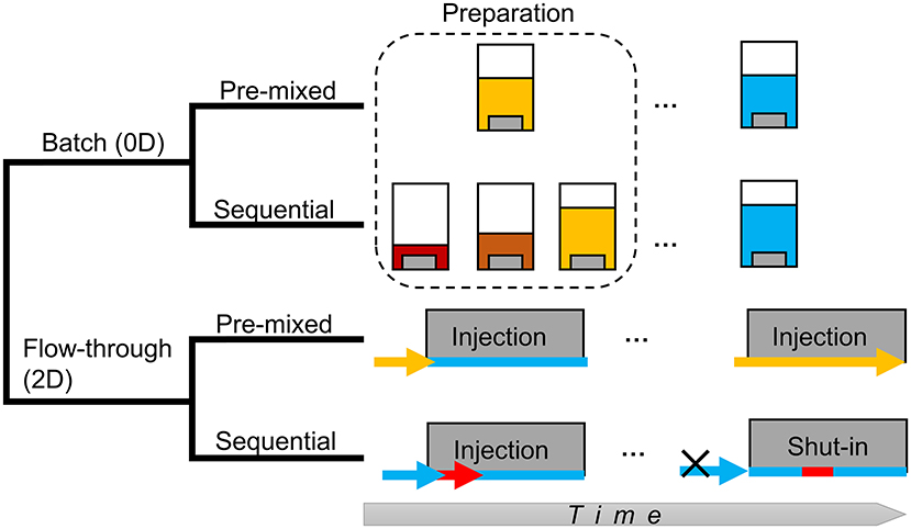
Figure 1. Schematics of models in this study. Solution acidity is illustrated by different colors. The warmer the color, the stronger the acidity. Concentrated HCl is shown in red, less concentrated HCl is orange, dilute acid (the pre-mixed condition) is yellow, and slickwater is blue.

The 2D model geometry is illustrated in Figure 2. It contains 298 by 92 grid cells to cover a 600 m by 10 m domain along x- and y-directions, respectively. This domain is large enough to capture the movement of injected acid and the resulting chemically altered zone of shale. The model has a primary fracture of 3 mm in aperture aligned along the long x-axis. Two minor fractures of 0.5 mm aperture connect perpendicularly to the primary fracture at x = 0.1 m and 200 m and extend along the y-axis. The fracture network is designed to simulate multiple scenarios in a single run. The vertical fracture at x = 0.1 m represents a location close to the injection point, whereas the one at x = 200 m is far from the injection point but close to where the acid spearhead resides when the shut-in period starts. In a benchtop core-flood experiment, the experimental system most resembles a region close to the injection point. From two locations (0.1 m downstream of each of the vertical fractures), as shown in Figures 2, 1D profiles along the y-axis direction were extracted from the 2D model output for mineral reaction analysis.

FIGURE 2

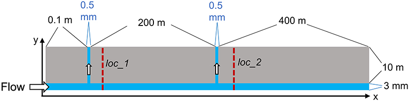
Figure 2. Illustration of the fracture layout for the 2D model. The illustration is not drawn in scale. All flow-through models were run for 7 days of reaction time. Loc_1 and Loc_2 refer to 1D profiles extracted from the 2D simulations for comparison.

The model grid cells were discretized to be finer close to the fracture where most of the reactions take place, and coarser away from the fractures. The finest grid cells are 5 μm, and the coarsest grid cells are 10 m. The fracture grid cells have an initial porosity of nearly 100%, compared to the shale grid cells with initial porosity of 5% (typical for shale). There is a layer composed of 5-μm-wide fluid-shale interfacial grid cells between the shale and fracture domains designed to enable efficient mass exchange across the shale-fluid interfaces as in the experimental system (Li et al., 2020). These interfacial grid cells contain a mixture of 50 vol% solution and 50 vol% shale matrix, yielding an overall porosity of 52.5%.

In all cases with flow, the flow rates in the primary fracture are set to be 10 times faster than that in the minor fractures. The flow rate in the primary fracture in the pre-mixed model is 0.001 m/s for the entire 7 days of simulation, whereas that in the sequential model it is 0.05 m/s and in total lasts for 85 min, with a 7-day no flow period afterward. The reaction time of 7 days is on the lower bound of typical shut-in periods of weeks (Wang et al., 2020; Khan et al., 2021; Jew et al., 2022) and is intended to encapsulate the time interval in which reactive alterations are most pronounced. Flow rates are determined so that the amount of HCl injected into the fracture in the pre-mixed and the sequential models are the same during the 7 days of reaction time. The flow velocity used in the pre-mixed model is several times higher than experimental values (Xiong et al., 2020). The flow velocity in the sequential model is likely to be slower than operational rates close to the injection point (Frackoptima, 2014). In real shale reservoirs, fluid velocity will decrease semi-radially from the injection point to remote volumes. To maintain reasonable computational burden, here we set flow velocities in the models to be constant. Under this setting, flow velocities are independent of pressure gradients and permeability, which are thus undefined.

Shale and solution compositions

In this study we examine mainly pH evolution as it reflects acid transport and pH neutralizing reactions. We also briefly analyze dissolution of calcite and precipitation of barite (BaSO₄) and iron (hydr)oxide [Fe(OH)₃] as examples of mineral reactions.

In our models, we specified typical shale and fluid compositions as the initial conditions, given in Tables 1, 2. The typical compositions are determined from prior experimental data (Dieterich et al., 2016; Harrison et al., 2017; Marcon et al., 2017; Vankeuren et al., 2017; Li et al., 2019b; Noël et al., 2020; Xiong et al., 2020; Khan et al., 2021). All systems are simulated at 80^oC.

TABLE 1

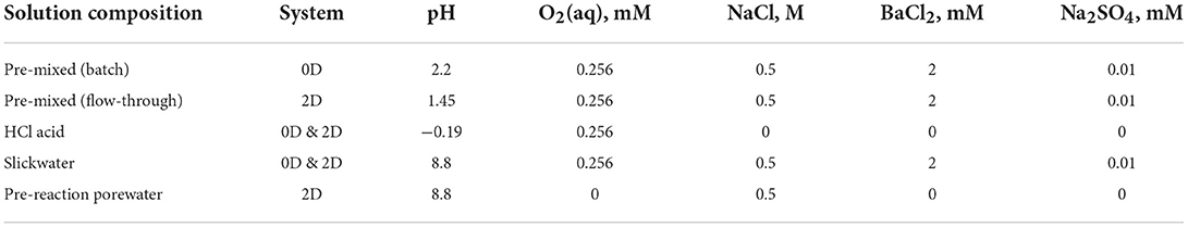
Table 1. Solution compositions used in this study.

TABLE 2

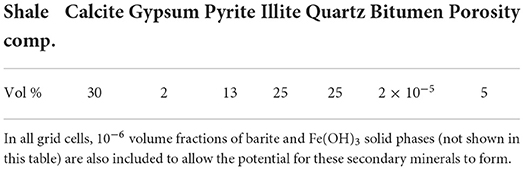
Table 2. Shale composition used in this study.

In the pre-mixed batch model, a hydrochloric (HCl) acid spearhead (i.e., a solution with 15 wt% of a 37 wt% HCl stock, equivalent to 5.6 wt% HCl) is assumed to be pre-mixed in a 100 mL solution to generate an initial pH of 2.2. In the pre-mixed 2D system, the pH of the pre-mixed solution is 1.45, which allows injection of the same overall amount of HCl as in the sequential model. An alternative method of defining equivalent acid delivery across our 2D simulations is to deliver HCl such that the effective H⁺ amounts (based on H⁺ activities) injected in both the pre-mixed and sequential systems are the same. This way of defining equivalent acid results in similar modeling results as those obtained in models with comparable overall amounts of HCl, as will be discussed in a later section.

The sequential models employ a solution addition schedule (Table 3) modified from typical pump schedules (Eberhard, 2011; Frackoptima, 2014; Li et al., 2016; Oilfieldbasics, 2019). A concentrated HCl acid (pH = −0.19) is added first, followed by several slickwater solutions with a pH of 8.8 in equilibrium with calcite at 80^oC. The slickwater contains 0.5 M NaCl and 0.256 mM dissolved O₂ (in equilibrium with atmospheric O₂ under ambient condition). 2 mM BaCl₂, and 0.001 mM Na₂SO₄ were also included to simulate commonly observed barite scale formation. The concentrations of barium and sulfate are appropriate representations of HFFs for barium rich reservoirs (Merdhah et al., 2007; Vankeuren et al., 2017). They generate mild saturation indices of log₁₀(Q/K_sp) = 1.25 in a “pre-mixed” solution and 1.29 in a “slickwater” solution (Table 1).

TABLE 3

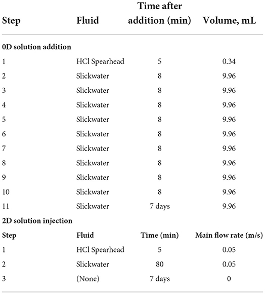
Table 3. Solution addition schedule used in the sequential models.

In both the batch and flow-through models, the shale is composed of 5 vol% porosity, 30 vol% calcite, 2 vol% gypsum, 13 vol% pyrite, 25 vol% illite, and 25 vol% quartz. It also contains bitumen to aid in Fe(II) oxidation, as specified in our previous studies (Jew et al., 2017; Li et al., 2019a). In the 2D geometry, the porosity is initially filled with porewater that has 0.5 M NaCl and a pH of 8.8 in equilibrium with calcite. The composition of porewater resembles the native formation water before any injections.

Initial secondary minerals

In the initial conditions in all grid cells, including the batch models, a very small amount (1 × 10⁻⁶ volume fraction) of barite and Fe(OH)₃ are also specified. These initial barite and Fe(OH)₃ amounts are necessary to provide the initial reactive surface areas required for secondary minerals to form if saturation conditions favor their formation. They will remain negligible if local conditions do not favor secondary mineral formation.

Chemical reaction network

The software package CrunchFlow is designed to simulate single-phase, multicomponent reactive transport phenomena in porous media at the continuum scale (Steefel et al., 2015). Both chemical reactions and transport are considered in the governing equation:

$\begin{array}{ll}\frac{\partial \phi C_i}{\partial t}=\frac{\partial }{\partial x}\left(D_{ie}\frac{\partial C_i}{\partial x}\right)-\frac{\partial }{\partial x}(\phi u{C}_i)-{\Sigma }_r{\nu }_{ir}{R}_{ir}& (1)\end{array}$

where C_i is the concentration of species i, φ is porosity, D_ie is the effective diffusion coefficient of species i, calculated according to Archie's law:

$\begin{array}{ll}{D}_{\text{ie}}={\phi }^m{D}_i& (2)\end{array}$

where m is the cementation exponent related to tortuosity, and D_i is the diffusion coefficient in bulk solution. In this study, m = 2.5 and D_i = 2 × 10⁻⁹ m/s² for all aqueous species, consistent with our previous modeling study (Li et al., 2020). In Equation 1, u is the advection velocity of the fluid, ν_irR_ir is the consumption of species i in the reaction r that has a rate of R_ir and a stoichiometric coefficient of ν_ir for species i.

Chemical reactions considered in this study include instantaneous aqueous speciation reactions dictated by equilibrium constants, and kinetic reactions that evolve with time according to a reaction rate calculated based on a given rate equation. Mineral kinetic reaction rates (mol/m³/s) follow the function:

$\begin{array}{ll}R=A•k•\prod {(a)}^n•(\frac{Q}{K_{sp}}-1)& (3)\end{array}$

where A is the mineral surface area (m²/g-mineral, convertible to m²/m³-porous medium) and k is the reaction rate constant (mol/m²/s). Because there are large uncertainties in both A and k, we collectively consider their variations in k by assigning 1 m²/g to A for all minerals. ∏(a)ⁿ is the product of all the activities of aqueous species exerting a rate dependence on the reaction, and Q and K_sp are the reaction quotient and solubility product, respectively. Aqueous kinetic rates (mol/kg-water/yr) are expressed in:

$\begin{array}{ll}R=k•\prod {(a)}^n•(\frac{Q}{K_{eq}}-1)& (4)\end{array}$

where k is the aqueous reaction rate constant, K_eq is the equilibrium constant of the reaction, and other parameters are the same as defined in Equation 3.

The methodology and model construction for Fe(OH)₃ formation pathways is detailed in our earlier work (Li et al., 2019a) and is summarized as follows: In the presence of oxidants, pyrite is oxidatively dissolved to release Fe(II) and sulfate (${\text{SO}}_4^{2-}$) into the aqueous phase. If excessive oxidants are present, Fe(II) can be further oxidized to Fe(III), which readily precipitates as Fe(OH)₃. Meanwhile, organic compounds in the HFF extract bitumen from shale, which catalyzes Fe(II) oxidation to Fe(III) by oxidants. The role of bitumen in Fe(II) oxidation, although currently unclear at the molecular level, is captured by an empirical rate law quantified in our previous study (Li et al., 2019a). In the current study, dissolved O₂ is the only oxidant. In operation, some biocides and breakers in the fracture fluid are also oxidants for Fe(II). In this study, almost all of the aqueous Fe in our study is in the Fe(II) form, because of the limited oxidant in our study, the preferential usage of O₂ by pyrite dissolution rather than Fe(II) oxidation, and the fast Fe(OH)₃ precipitation that removes Fe(III) form solution.

A detailed reaction network was specified in our previous modeling studies (Li et al., 2019a, 2020). In this current study, we used a slightly simplified reaction network as shown in Table 4. The equilibrium constants at 80 ^oC were interpolated using values at multiple temperature points in the CrunchFlow database. For mineral reactions, we examine only calcite dissolution, barite precipitation, and Fe(OH)₃ formation. The effects of acidic fluids on dissolution of minerals other than calcite are minor at the modeling timescale.

TABLE 4

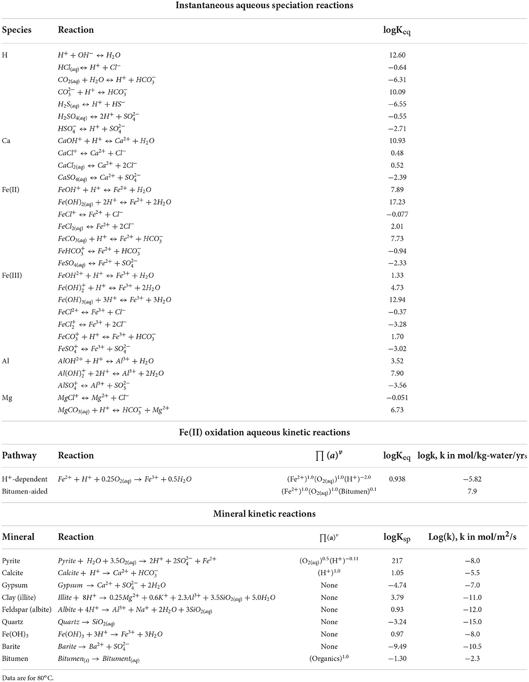
Table 4. Reaction network in the model.

Modeling method—Batch system

In these simulations we assume that the system is homogeneous, well-mixed, and there is no consideration of transport. Under this assumption, the model was setup following a typical experimental design where 1 g of crushed shale was reacted with a 100 mL solution (Harrison et al., 2017; Jew et al., 2017). In the 0D grid cell with 100 mL volume, assuming a shale density of 2.5 g/cm³, the volume of shale is 0.40 cm³. Considering the whole reactor as a porous media, the porosity is near 100%. In the pre-mixed model, the pore space is filled with the pre-mixed solution specified for the batch system (Table 1).

In the sequential batch model, reaction solutions were introduced in multiple steps, resulting in an evolving fluid: solid ratio in each step of the addition process. To simulate this sequential protocol, additional method development was performed as follows. In the first step, the shale sample reacts with 0.34 mL concentrated acid for 5 min. In this step, the 0.40 cm³ shale takes 54% of the total volume, with the rest of the total “porous media” volume occupied by HCl acid. The HCl acid is a 5.6 wt% HCl solution, equivalent to 1.8 M HCl, with a calculated pH of −0.19. We note this presents a rare situation for the software in that the pH starts at a negative value and passes 0 to become positive over the dissolution process. Typically, software such as CrunchFlow uses H⁺ as a “master variable” in that the rate of change of the H⁺ activity in solution dictates the maximum allowable timestep in the model. Given the extremity with which this parameter changes in our simulations, we switch the mater variable to Ca²⁺ that is actively changing, but in a more reasonable manner than pH. The model for the acid spearhead step was run for a duration of 5 min.

To setup the model for the next step with 8 ml of additional slickwater (Table 3), the 5 min model outputs were pulled to write the new initial conditions for the second simulation. The required outputs are the total aqueous concentrations and total mineral volumes. Total aqueous concentrations incorporate all species required to construct the exact aqueous condition (Morel and Hering, 1993). The concentrations in the input file for the second simulation consider two parts: (i) Dilution of each species' total concentration by the new addition of slickwater, and (ii) any corresponding dilution of species in the newly added slickwater.

In addition to total concentrations, each subsequent initial condition also requires mineral volume fractions. From the first step model outputs, mineral fractions are obtained. With slickwater added in the system, these mineral volume fractions reduce such that the fluid: solid ratio increases. The barite and Fe(OH)₃ amounts, although negligible in their volume fractions, must be further adjusted to match those in the pre-mixed model. They are adjusted in each step by assuming that the newly added slickwater has 1 × 10⁻⁶ volume fractions of barite and Fe(OH)₃, which are then diluted and mixed into the system. The aqueous and solid compositions from the earlier step and the newly added slickwater were combined to form the initial condition in the next step. This calculation was done for each subsequent step in the sequential model.

Reaction times of each step were summed up to obtain the entire duration of the numerical experiment. For example, the second step was run to obtain the 8 min output results (Table 3), which is equivalent to a total reaction time of 13 min, the sum of 5 min in the first step and 8 min in the second step. In the last step, the model runs for a longer time (Table 3) to obtain the 7-day results.

The overall process of pulling the output from each step, conducting dilution calculations to obtain the initial conditions for the next step, and simulating the next step was accomplished using a Python script. Both CrunchFlow input files and the python script are available in the Supporting Information.

Modeling method—Flow-through system

The initial 2D model has a 5% porosity in the shale grid cells, a ~100% porosity in the fracture grid cells, and a 52.5% porosity in the narrow interfacial layer of grid cells between shale and fracture domains. These porosity spaces are filled with pre-reaction porewater fluid (Table 1), representing the native system prior to injection of any acid or fracturing fluids. As explained earlier, all grid cells in the initial condition contain 1 × 10⁻⁶ volume fractions of barite and Fe(OH)₃ as potential secondary precipitates. In the pre-mixed model, the pH 1.45 pre-mixed solution is injected from the left of the main fracture for the entire 7 days of reaction time. In the sequential-injection model, the pH −0.19 acid spearhead is injected through the main fracture for 5 min, corresponding to the concentrated HCl addition step in Table 3. Slickwater is then injected for another 80 min, equivalent to the total time of slickwater additions in the batch reactor (steps 2-11 with 8 min assigned to the last addition), after which flow is set to zero for the remainder of the 7 days. The overall sequential injection takes three input files, given that the model geometry does not change and only input injection concentrations and flow velocities alter. This is achieved with the restart function built into CrunchFlow.

Results and discussion

Batch system

Time-resolved modeling results for pH and selected solutes are shown in Figure 3. Overall, concentration time-series in the sequential model change more dramatically than those in the pre-mixed system. However, the difference becomes negligible after the first day.

FIGURE 3

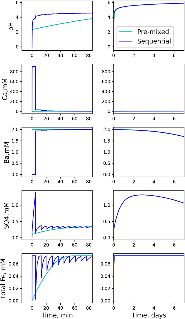
Figure 3. Aqueous compositions modeled with pre-mixed and and sequential protocols in a 0D batch system. Due to low water-to-rock ratios and strong acidity in the initial steps in the sequential model, the concentrations at early time change dramatically relative to the pre-mixed model. After several hours, the two models have similar concentrations.

Both pH and Ca²⁺ evolutions are more dramatic in the sequential model, as a result of the concentrated acid and low water-to-rock ratios at the beginning steps of the simulation. The concentration of Ca²⁺ increases due to dissolution of calcite and gypsum:

$\begin{array}{ll}CaC{O}_3(calcite)+H^{+}=C{a}^{2+}+HC{O}_3^{-},and& (5)\end{array}$

$\begin{array}{ll}CaS{O}_4·2H_{2}O(gypsum)=C{a}^{2+}+S{O}_4^{2-}+2H_{2}O& (6)\end{array}$

Calcite dissolution consumes H⁺, resulting in increasing pH. As additional solution with no HCl is subsequently added into the batch system, both acidity and Ca²⁺ are diluted over multiple steps, resulting in a decrease in Ca²⁺ and increase in pH.

The difference in barium concentrations at early stages between the pre-mixed and the sequential models is due to the lack of Ba²⁺ in the acid spearhead in the sequential model, whereas barium is included in the pre-mixed solution.

${\text{SO}}_4^{2-}$ is a component in slickwater (Table 1), and is also generated from both gypsum dissolution (Equation 6) and pyrite oxidation:

$\begin{array}{ll}Fe{S}_2(pyrite)+3.5O_2(aq)+H_{2}O=F{e}^{2+}+2S{O}_4^{2-}+2H^{+}& (7)\end{array}$

In the early steps of the sequential model (Table 3), the acidic solution volume is small relative to shale volume, such that the initial calcium and sulfate concentrations increase rapidly. With subsequent dilution by additional slickwater additions, they begin to stabilize. Barite precipitation removes Ba and sulfate from the solution according to:

$\begin{array}{ll}B{a}^{2+}+S{O}_4^{2+}=BaS{O}_4(barite)& (8)\end{array}$

The declining curves of the barium and sulfate concentrations in Figure 3 show that barite precipitation starts after 2 days in our models, with no systematic differences between the pre-mixed and the sequential models.

The total Fe concentration in the sequential model approaches almost the same equilibrium plateau in each step. Fe(II) is released by oxidative dissolution of pyrite, which can be oxidized to Fe(III) if additional oxidants are available. Because dissolved oxygen is limited in our system and because Fe(III) readily forms Fe(OH)₃ solid, Fe(III) remains negligible in the aqueous phase compared to Fe(II) throughout the reaction. The stabilized Fe concentrations in each step are similar when dissolved oxygen is > 98% depleted. This is a result of the fact that in all solutions added to the system, including the acid spearhead, the dissolved O₂ has the same concentration.

After all portions of slickwater are added in the sequential model, concentrations from the sequential model and the pre-mixed model converge to comparable values on the time scale of days. One caveat of this conclusion is that it is based on the assumption that the system is well-mixed and homogeneous. In the experiments with sequential additions of fracturing fluids, it is possible that some concentrated HCl gets trapped in shale pores and affects the system for longer periods of time than predicted for a well-mixed system. Another caveat is that such concentrated HCl can potentially trigger mineral reactions that are not currently described in the model, such as leaching of specific ions only when pH is extremely low (Noël et al., 2020). Future experiments focused on identification and quantification of these water-shale interactions in the presence of concentrated HCl would be valuable. Without a priori knowledge of these potentially missing reactions, the experimental protocol with a pre-mixed solution at pH 2.2 is a reasonable approximation of a sequential addition protocol when designing a batch experiment (Harrison et al., 2017; Jew et al., 2017; Li et al., 2019b; Noël et al., 2020).

Flow-through system—pH

Unlike the batch system, the flow-through geometry exhibits an obvious difference between the sequential and the pre-mixed models over the 7-day simulations. Injection of the pre-mixed solution drives a pH gradient that gradually extends into the surrounding shale matrix by 1–3 cm, depending on the distance from the injection point, as shown in Figures 4A–E. The acid is gradually neutralized along the flow path (0.001 m/s flow rate in the horizontal main fracture) by calcite dissolution, reaching a pH of 5.0 in the first 50 m after injection. Although the pH is still relatively low, it is in equilibrium with calcite. This is because CO₂ generated from calcite dissolution is not allowed to degas in the model, which is likely to be the case in the high-pressure subsurface. The aqueous CO₂ forms carbonic acid with water, reducing the equilibrium pH. As aqueous CO₂ diffuses into surrounding grid cells (in the shale matrix) downstream, CO₂ concentration becomes lower in the fracture and the equilibrium pH slightly increases. At 600 m on the x-axis, the fracture pH is 5.8 at Day 7. With the pre-mixed injection, observable reactive alteration occurs only close to the injection point. In the upstream fine fracture (0.5 mm aperture), the acid is quickly neutralized (Figure 4F). The downstream fine fracture experiences a pH change (Figure 4G), but there is no observable calcite dissolution (as will be shown later), because the solution is already saturated with calcite when it arrives at this downstream vertical fracture.

FIGURE 4

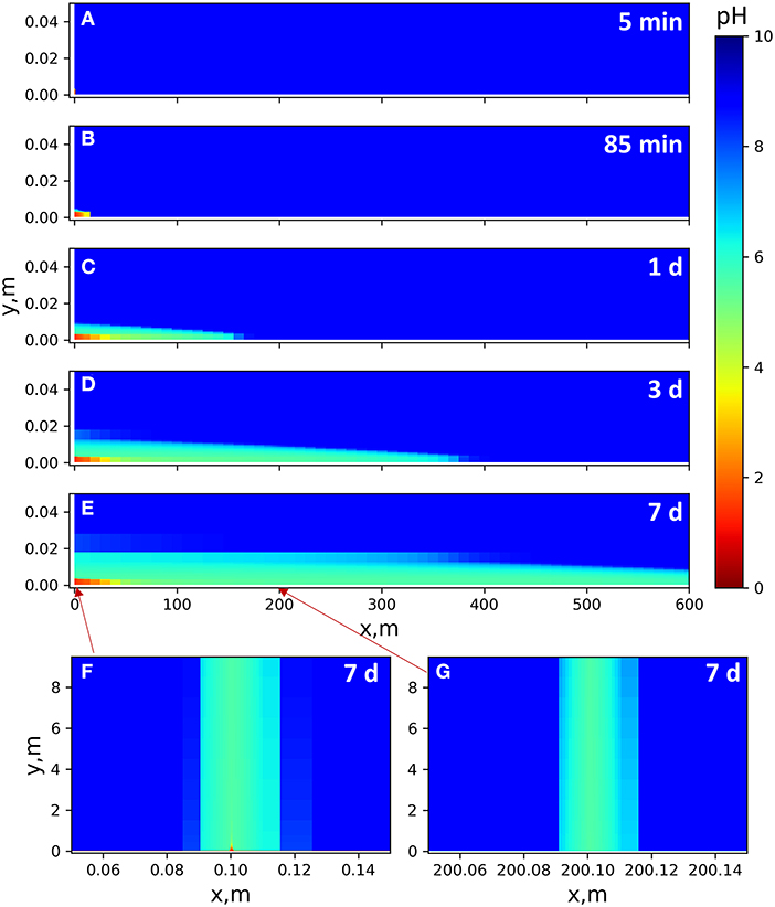
Figure 4. pH gradients in the 2D pre-mixed models with continuous injection of a pH 1.45 solution. There is no flow in the shale matrix. pH gradients in the shale matrix are due to ion diffusion. (A–E) Time-resolved results for pH alteration close to the main fracture (y direction shown up to 5 cm). Injection point: (0, 0). Fracture width: 3 mm. Flow rate: 10⁻³ m/s. (F,G) pH altered zones after 7 days of reaction along vertical fractures close to and far from the injection point, respectively. Mapped for the entire y domain 0–10 m. Fracture width: 0.5 mm. Flow rate: 10⁻⁴ m/s.

In the sequential-injection model (Figure 5), if we were to assume perfect plug flow (no mixing) and an inert fluid, the spearhead would reach a location in the main fracture of x = 240–255 m at the end of injection and beginning of shut-in. When we do include both the neutralizing mineral reactions and diffusive mixing, the spearhead affects a much larger spatial zone, spreading 100–450 m on the x-axis of the main fracture. Across this width, the acid diffuses into the shale matrix and forms as much as a 3 cm deep zone of pH gradients.

FIGURE 5

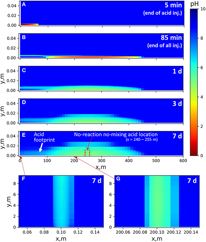
Figure 5. pH gradient in the 2D sequential model at the end of selected overall reaction times (injection time included). There is no flow in the shale matrix domains. pH gradients in the shale matrix are due to ion diffusion. (A–E) Time-resolved results close to the main fracture (y direction shown up to 5 cm). Injection point: (0, 0). Fracture width: 3 mm. Flow rate: 0.05 m/s for time = 0–85 min, no flow afterward. (F,G) pH results after 7 days of reaction in vertical fractures close to and far from the injection point, mapped for the entire y domain. Fracture width: 0.5 mm. Flow rate: 0.005 m/s for 0–85 min, no flow afterward.

As the acid spearhead travels in the fracture during injection, the concentrated acid diffuses into the shale matrix, resulting in continued expansion of the pH gradient in the shale matrix even after the spearhead passes by. In this model, diffusion is the only mixing mechanism within the shale interior. With advective mixing, the affected zone could be wider.

Calcite dissolution neutralizes acid and counteracts the depth of acid penetration into the shale. If the 30 vol% calcite content used in the model were lowered, the acid would spread faster in the fractures, and acid neutralization becomes much slower (Figure 6). In an extreme case where there are no mineral reactions, the acid quickly spreads across the entire 600 m x-axis domain. The depths of acid diffusion into the matrix are similar in Figures 5, 6, because on the mm–cm scale, the effective diffusion remains a limiting factor despite calcite dissolution. The alteration in porosity, which largely determines alteration in effective diffusion, extends several millimeters into the shale matrix, much narrower than the pH-affected zone, as will be discussed later.

FIGURE 6

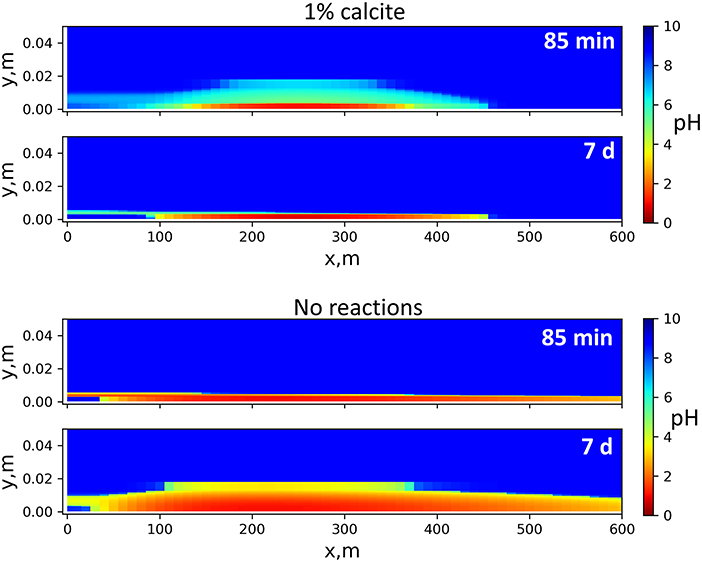
Figure 6. pH distribution in the 2D flow-through sequential model assuming either 1 vol% calcite (Top) or no mineral reactions (Bottom). With low calcite in shale, acid neutralization is slower. If no mineral reactions are considered, the acid quickly spreads over the entire main fracture length and slowly diffuses into the shale matrix through pore spaces.

Flow-through system—Mineral reactions

To compare mineral reactions in the 2D pre-mixed and sequential systems, 1D profiles were generated along the y-direction (Figure 2). The 1D transects are positioned 10 cm downstream of the vertical fractures. Transect location #1 (loc_1) is close to the injection point (0.2 m down the main fracture length), and the transect location #2 (loc_2) is 200 m down the main fracture length from the injection point. These 1D profiles for the pre-mixed and sequential scenarios are shown in Figure 7.

FIGURE 7

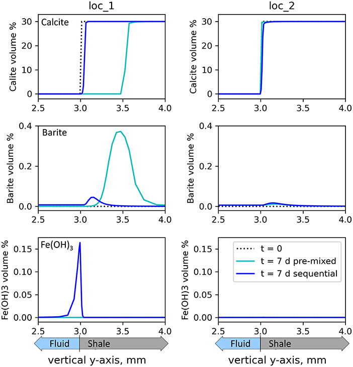
Figure 7. Mineral volume percentages along vertical 1D transects at location #1 (loc_1, 0.2 m from injection point) and location #2 (loc_2, 200 m from injection point) in the 2D pre-mixed and sequential flow-through models. The transect locations are illustrated in Figure 2. The fluid-shale interface is positioned at 3.00 mm on the horizontal axis (which denotes the y axis in the 2D model), with fracture fluid on the left and shale matrix on the right. In the pre-mixed model, both calcite dissolution and barite precipitation occur more noticeably at loc_1 than loc_2. Fe(OH)₃ precipitation is negligible. In the sequential model, calcite dissolution occurs at both locations with narrow reaction zones. Barite precipitation also occurs at both locations, inside the shale matrix. Fe(OH)₃ precipitates in the fracture space and only at loc_1.

In the pre-mixed model (Figure 7), both calcite dissolution and barite precipitation are more pronounced closer to the injection point than further down the main fracture length. In fact, calcite dissolution downstream is negligible. This is because the upstream fracture is always exposed to newly injected acid, Ba²⁺, and ${\text{SO}}_4^{2-}$. Calcite dissolution and barite precipitation are thus very localized to the injection point. This upstream reaction zone is represented by a typical benchtop core-flood setup, where a fresh solution is continuously injected into a relatively short core. The absolute size of the obvious calcite-dissolving region in the pre-mixed model is dependent on the flow rate. If the constant flow rate were set higher (with lower HCl concentration to maintain the total HCl amount), this region would extend a longer distance along the flow-direction and the local maximum calcite dissolution would be less intensive.

In our model system, ${\text{SO}}_4^{2-}$ is present in the slickwater and is also generated by gypsum dissolution, which is most prolific close to the injection point, i.e., where fluid is more undersaturated. Sulfate generated from oxidative pyrite dissolution is minor compared to that from gypsum. Because of the relatively high barium and sulfate concentrations at the injection point, barite precipitation is more obvious at loc_1 than loc_2. Barite prefers to form in the matrix because the matrix has more gypsum than the fracture to release the limiting species, ${\text{SO}}_4^{2-}$, to the aqueous phase. At loc_2, away from the injection zone, a small volume of barite has begun to precipitate in the main fracture itself, because dissolution of pyrite and gypsum (mainly gypsum) along the flow path has accumulated ${\text{SO}}_4^{2-}$, resulting in more favorable conditions for barite precipitation. Fe(OH)₃ precipitation is not noticeable at both locations, because the flow continuously flushes Fe downstream (mostly Fe²⁺), where dissolved oxygen is depleted by pyrite dissolution, allowing no local Fe³⁺ accumulation to precipitate noticeable Fe(OH)₃ amounts.

In the sequential model (Figure 7), calcite dissolution is observable in both locations but to a far less significant extent than loc_1 in the pre-mixed model. The comparison suggests that in the sequential model, calcite dissolution occurs over a longer length-scale through the fracture.

Because calcite dissolution is the main reason for porosity changes, the trend of calcite dissolution is also observable from porosity changes. As shown in Figure 8, an obvious porosity increase is observable close to the injection point in the pre-mixed model, but is widely distributed along the flow path in the sequential model. The integrated secondary porosity changes in the two systems are controlled by the stoichiometric relationship between H⁺ and calcite according to Equation 5. With the same amount of HCl injected into the two systems (which are almost all deprotonated to H⁺ and Cl⁻), the integrated secondary porosities of the two simulations are expected to be similar. Barite and Fe(OH)₃ accumulation contributes little to porosity changes, although they may obviously change permeability if formed in pore-throats.

FIGURE 8

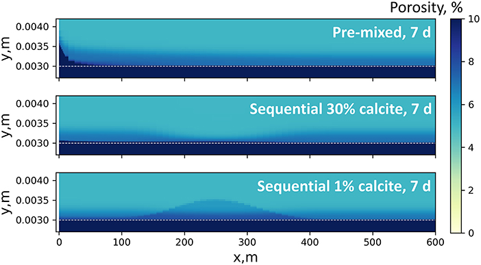
Figure 8. Porosity maps of the pre-mixed and sequential 2D models after 7 days of overall reaction time. Note that the y-axis range is much narrower than that in the pH maps. The white dotted line denotes the location of the fracture surface. Porosity increase (fracture opening, dark blue zones) is mostly observable in the pre-mixed model close to the injection point. In the sequential model with 30% calcite, porosity increase occurs along the fracture path. Minor porosity increase is observed in shale matrices in all cases due to diffusion of acid into the shale matrix. Porosity map of the sequential system with a lower calcite content shows a distinct pattern of porosity alteration: porosity increase is most observable close to where the concentrated HCl stops at the beginning of the no-flow shut-in stage. This demonstrated the dependence of spatial distribution of mineral reactions on mineralogy composition.

The relative amounts of calcite dissolution at up- and down-stream locations in the sequential model heavily depend on the shale mineral composition. The 30% calcite content in our model supports extensive dissolution, which consumes much of the acidity before the acid spearhead reaches loc_2, resulting in limited dissolution and porosity opening at loc_2. If the matrix calcite content is very low (e.g., 1% calcite), the acid spearhead in the sequential model is only slightly neutralized before shut-in begins, such that an obvious calcite-dissolution/porosity-opening zone develops at the location where the acid spearhead is placed during shut-in (Figure 8).

In the sequential model, barite precipitation is also well-distributed along the x-axis, with both upstream and downstream barite in mild amounts. The barite volume at loc_1 close to injection point is slightly higher than that at loc_2 far from the injection point, but this comparison is subject to shale and fluid compositions. For example, in a high-barium low-sulfate formation, as in our model, sulfate is the limiting species for barite formation. If no sulfate anions are produced from chemical reactions along the flowpath (e.g., from decomposition of persulfate breakers, pyrite dissolution, and gypsum dissolution), barite precipitation close to the injection point would consume all sulfate anions, resulting in no barite precipitation downstream. Alternatively, if sulfate anions are produced by chemical reactions along the flow path, it is also possible that significant barite forms downstream. In addition, if there are colloidal barite particles with considerable reactive surface areas in the fracture, barite precipitation in the fracture is expected to be more extensive (Jew et al., 2017; Li et al., 2020; Spielman-Sun et al., 2021).

Fe(OH)₃ precipitation occurs mainly in the fracture close to the injection point, where the dissolved oxygen is most available. Dissolved oxygen can dissolve pyrite, releasing Fe(II). As there is no flow during shut-in, the O₂ level close to the inlet can further oxidize Fe(II) to Fe(III), which accumulates locally until Fe(OH)₃ solids are formed.

Acid reactivity in concentrated solutions

As discussed in the earlier section, the apparent differences of the 2D pre-mixed and the sequential models were attributed to differences in the injection pattern, as both systems received the same total amount of HCl over the 7 days of reaction time. However, it is worth noting that the H⁺ activity (i.e., effective H⁺ concentration) can be quite different from the actual concentration in solutions with high ionic strength, as in our modeling cases. Under these conditions, the activity of an aqueous ion is usually expected to be lower than the true concentration because the ion is surrounded by ions with opposing charge, which effectively shields the apparent charge of the center ion in solution (Benjamin, 2014).

The CrunchFlow software uses the extended Debye-Hückel equation to calculate the ion activities (Helgeson et al., 1969; Steefel et al., 2015). Although the calculation is most trusted up to 1 M ionic strength, it nonetheless provides insights into the reactivity of chemicals in our solutions. In our solutions virtually all HCl dissociates into H⁺ and Cl⁻. However, the high ionic strength of the 1.8 M solution produces an H⁺ activity of only 1.534 M (activity coefficient = 0.852). Similarly, the 2D pre-mixed solution has a 0.56 M ionic strength provided mostly by NaCl. The activity of H⁺ in this scenario is 3.53 × 10⁻² M in comparison to the actual H⁺ concentration of 4.50 × 10⁻² M (activity coefficient = 0.785). Hence it is possible that the 2D pre-mixed and sequential models received the same overall HCl but did not experience the same effective H⁺ amount at these high ionic strengths.

To evaluate this effect, we ran an additional 2D pre-mixed simulation with adjustment of the HCl concentration so that the same effective H⁺ amount is delivered as in the sequential models. The injected solution has an HCl concentration of 4.88 × 10⁻² M, and the corresponding H⁺ activity is 3.84 × 10⁻² M, which yields a pH of 1.42 (activity coefficient = 0.794). We find that the results of this adjusted model (Supplementary Figures 1, 2) do not apparently differ from those presented in Figures 4, 7, and hence the injection patterns rather than the differences in H⁺ activities and concentrations appear to produce the unique behavior among our simulations.

Connecting bench-top experiments and field applications

Reactive transport models have been used extensively to quantify coupling of reactivity and transport porous media (Druhan et al., 2019). Calibration of the models with experimental data validates the model and decodes important mechanisms (Deng et al., 2017; Li et al., 2017; Meile and Scheibe, 2019; Ling et al., 2020; Jew et al., 2022). The calibrated models can then serve as tools to explore a wider range of scenarios including unique reaction conditions or extended temporal/spatial scales (Xu et al., 2010; Esteves et al., 2022). The model framework used in this study has been calibrated with experimental observations in our previous work (Li et al., 2020).

Of the two reactive transport systems considered in this study, the pre-mixed model shows obvious reactions (both dissolution and precipitation) close to the injection point. This prediction is consistent with core-flood experimental studies where extensive reactions are observed either close to the injection point or over the entire core (corresponding to the “close-to-injection” scenario in our pre-mixed model) (Deng et al., 2015, 2017; Vankeuren et al., 2017; Xiong et al., 2021a). In contrast, our sequential-injection reactive transport model demonstrates that the spatial distributions and extents of reactions in the fracture domain are dependent on water and rock compositions as well as injection patterns. There is currently no experimental data available for such a sequential injection scenario, though this practice is widely applied in hydraulic fracturing operations. One challenge with such experiments is the limited size of a bench-scale setup. This is potentially resolvable via new designs of flow-through setups, such as that used in Wolterbeek et al. (2016), where cement-filled tubes of 1–6 m long captured flow paths longer than typical flow-through setups. Although creating an explicit fracture geometry in a similar system is difficult, it is possible to use a long tube packed with shale grains to examine water-rock interactions over a long flow path. Another limitation is the strongly corrosive nature of concentrated HCl on high-pressure experimental equipment if the consecutive injection schedule is to be applied. To avoid damage to instrumentation, an approximate approach, as performed in Xiong et al. (2021b), involves treatment of the shale sample by concentrated HCl prior to setting up the full flow-through system. Alternatively, sequential injection experiments can be carried out with diluted HCl. The diluted acid will result in mitigated geochemical reactions, but could still provide insights into spatial distributions of reactions relative to the stagnant location of the acid spearhead during shut-in. As discussed earlier for the batch system, there might be potential geochemical reactions that can be triggered by HCl only when it is concentrated. These reaction mechanisms can be separately investigated in a batch reactor and incorporated into a flow-through system through the use of reactive transport models such as we have demonstrated here.

Our study demonstrates that injection patterns should be considered when interpretating bench-top experimental data as well as field observations. For example, a large porosity increase/decrease in a core-flood experiment may not quantify the extent or spatial distribution of porosity alteration in an authentic operating system that experiences sequential injections. Overall, the current study sets a start point for improved understanding among laboratory experimentalists and field operators, and between academia and industry.

Conclusions

In this study we constructed 0D and 2D numerical models to compare two experimental protocols used to study shale-fluid interactions: (1) starting the reaction with an acidic solution at pH ~2, assuming that the concentrated acid spearhead is pre-mixed with slickwater; and (2) introducing the concentrated acid and slickwater to the shale system separately in sequential steps. Models were setup for both batch systems and flow-through systems. The flow-through system is extended to field scale fractured shale domains.

We found that in the batch system, the sequential protocol will generate much more dramatic changes in aqueous concentrations in early stages. After the first few hours, as the concentrated solution in the sequential model is diluted by slickwater, the two protocols produce similar results.

In the flow-through system, we found that with a pre-mixed protocol, most reactions occur close to the injection point. With a sequential protocol, the spatial distribution of reactions depends on the location of the acid spearhead during the shut-in stage. In our case, calcite dissolution and barite precipitation distributed along a greater length along the fracture compared to the pre-mixed model. Detailed results are also dependent on the specific mineralogy and fluid composition of a given system. In both the pre-mixed and the sequential models, calcite dissolution can neutralize the injected acid to a pH of 5–6, in equilibrium with calcite but lower than the formation pH because of the carbonic acid produced during calcite dissolution. Comparison between the results obtained from the two injection protocols highlights the importance of consideration of not only the amount of chemicals injected down a well or into a fracture, but also the sequence and injection schedule, which can lead to dramatic different spatial and temporal distributions of geochemical reactions in the geomedia.

These findings provide insight into the design and evaluation of experimental results obtained from laboratory settings, and also guide application of experimental findings to interpreting data and improving practices in industrial settings.

Data availability statement

The original contributions presented in the study are included in the article/supplementary material, further inquiries can be directed to the corresponding authors.

Author contributions

QL generated the research idea, did the modeling work, and wrote/revised the manuscript. JLD participated in discussions during the study and provided constructive suggestions for revision. JRB oversees the whole project and participated in discussions and paper revisions. All authors contributed to the article and approved the submitted version.

Funding

This study was funded by the U.S. Department of Energy, Office of Fossil Energy, Office of Oil and Natural gas to SLAC under Contract No. DE-AC02-76SF00515. The Stanford Synchrotron Radiation Lightsource, a directorate of SLAC, was supported by the U.S. Department of Energy, Office of Science, Office of Basic Energy Sciences.

Conflict of interest

The authors declare that the research was conducted in the absence of any commercial or financial relationships that could be construed as a potential conflict of interest.

Publisher's note

All claims expressed in this article are solely those of the authors and do not necessarily represent those of their affiliated organizations, or those of the publisher, the editors and the reviewers. Any product that may be evaluated in this article, or claim that may be made by its manufacturer, is not guaranteed or endorsed by the publisher.

Supplementary material

The Supplementary Material for this article can be found online at: https://www.frontiersin.org/articles/10.3389/frwa.2022.998379/full#supplementary-material

References

Ajo-Franklin, J., Voltolini, M., Molins, S., and Yang, L. (2018). “Coupled processes in a fractured reactive system: a dolomite dissolution study with relevance to gcs caprock integrity,” in Geological Carbon Storage: Subsurface Seals and Caprock Integrity (Hoboken, NJ: John Wiley and Sons), 187–205. doi: 10.1002/9781119118657.ch9

CrossRef Full Text | Google Scholar

Benjamin, M. M. (2014). Water Chemistry. Long Grove, IL: Waveland Press.

PubMed Abstract | Google Scholar

Crawley, G. M. (2016). Fossil Fuels: Current Status and Future Directions. World Scientific Series In Current Energy Issues. World Scientific Publishing Company. doi: 10.1142/9698

CrossRef Full Text | Google Scholar

Deng, H., Fitts, J. P., Crandall, D., Mcintyre, D., and Peters, C. A. (2015). Alterations of fractures in carbonate rocks by CO2-acidified brines. Environ. Sci. Tech. 49, 10226–10234. doi: 10.1021/acs.est.5b01980

PubMed Abstract | CrossRef Full Text | Google Scholar

Deng, H., Voltolini, M., Molins, S., Steefel, C., Depaolo, D., Ajo-Franklin, J., et al. (2017). Alteration and erosion of rock matrix bordering a carbonate-rich shale fracture. Environ. Sci. Tech. 51, 8861–8868. doi: 10.1021/acs.est.7b02063

PubMed Abstract | CrossRef Full Text | Google Scholar

Dieterich, M., Kutchko, B., and Goodman, A. (2016). Characterization of marcellus shale and huntersville chert before and after exposure to hydraulic fracturing fluid via feature relocation using field-emission scanning electron microscopy. Fuel 182, 227–235. doi: 10.1016/j.fuel.2016.05.061

CrossRef Full Text | Google Scholar

Druhan, J., Tournassat, C., and America, M. S. O. (2019). “Reactive transport in natural and engineered systems,” in Mineralogical Society of America, Vol. 85, eds J. Druhan and C. Tournassat. doi: 10.1515/9781501512001

CrossRef Full Text | Google Scholar

Eberhard, M. (2011). Fracture Design and Stimulation – Monitoring. US EPA. Available online at: https://www.epa.gov/sites/default/files/documents/fracturedesignandstimulationmonitoring.pdf (accessed on March 17, 2022).

Google Scholar

Esteves, B. F., Spielman-Sun, E., Li, Q., Jew, A. D., Bargar, J. R., and Druhan, J. L. (2022). Geochemical modeling of celestite (SrSO4) precipitation and reactive transport in shales. Environ. Sci. Tech. 56, 4336–4344. doi: 10.1021/acs.est.1c07717

PubMed Abstract | CrossRef Full Text | Google Scholar

Fan, W., Hayes, K. F., and Ellis, B. R. (2018). Estimating radium activity in shale gas produced brine. Environ. Sci. Tech. 52, 10839–10847. doi: 10.1021/acs.est.8b01587

PubMed Abstract | CrossRef Full Text | Google Scholar

Frackoptima (2014). Pumping Schedule. Frackoptima Inc. Available online at: http://www.frackoptima.com/userguide/interface/pumping-tab.html#fig-pumping-schedule (accessed March 17, 2022).

Google Scholar

Frackoptima (2017). Pumping Schedule. Available online at: http://www.frackoptima.com/userguide/interface/pumping-tab.html (accessed May 26, 2022).

Google Scholar

Gundogar, A. S., Druhan, J. L., Ross, C. M., Jew, A. D., Bargar, J. R., and Kovscek, A. R. (2021). “Core-flood effluent and shale surface chemistries in predicting interaction between shale, brine, and reactive fluid,” in SPE/AAPG/SEG Unconventional Resources Technology Conference: OnePetro (Houston, TX). doi: 10.15530/urtec-2021-5640

CrossRef Full Text | Google Scholar

Harrison, A.L., Jew, A.D., Dustin, M.K., Thomas, D.L., Joe-Wong, C.M., Bargar, J.R., et al. (2017). Element release and reaction-induced porosity alteration during shale-hydraulic fracturing fluid interactions. Appl. Geochem. 82, 47–62. doi: 10.1016/j.apgeochem.2017.05.001

CrossRef Full Text | Google Scholar

Helgeson, H. C., Garrels, R. M., and Mackenzie, F. T. (1969). Evaluation of irreversible reactions in geochemical processes involving minerals and aqueous solutions—II. Applic. Geochimica et Cosmochimica Acta 33, 455–481. doi: 10.1016/0016-7037(69)90127-6

CrossRef Full Text | Google Scholar

Herz-Thyhsen, R. J., Miller, Q. R., Rother, G., Kaszuba, J. P., Ashley, T. C., Littrell, K. C. J., et al. (2021). Nanoscale interfacial smoothing and dissolution during unconventional reservoir stimulation: implications for hydrocarbon mobilization and Transport. ACS Appl. Mater. Interfaces 13, 15811–15819. doi: 10.1021/acsami.0c22524

PubMed Abstract | CrossRef Full Text | Google Scholar

Jew, A.D., Druhan, J.L., Ihme, M., Kovscek, A.R., Battiato, I., Kaszuba, J.P., et al. (2022). Chemical and reactive transport processes associated with hydraulic fracturing of unconventional oil/gas shales. Chem. Rev. 122, 9198–9263. doi: 10.1021/acs.chemrev.1c00504

PubMed Abstract | CrossRef Full Text | Google Scholar

Jew, A.D., Dustin, M.K., Harrison, A.L., Joe-Wong, C.M., Thomas, D.L., Maher, K., et al. (2017). Impact of organics and carbonates on the oxidation and precipitation of iron during hydraulic fracturing of shale. Energy Fuels 31, 3643–3658. doi: 10.1021/acs.energyfuels.6b03220

CrossRef Full Text | Google Scholar

Khan, H. J., Ross, C. M., and Druhan, J. L. (2022). Impact of concurrent solubilization and fines migration on fracture aperture growth in shales during acidized brine injection. Energy Fuels 36, 5681–5694. doi: 10.1021/acs.energyfuels.2c00611

CrossRef Full Text | Google Scholar

Khan, H. J., Spielman-Sun, E., Jew, A. D., Bargar, J., Kovscek, A., and Druhan, J. L. (2021). A critical review of the physicochemical impacts of water chemistry on shale in hydraulic fracturing systems. Environ. Sci. Tech. 55, 1377–1394. doi: 10.1021/acs.est.0c04901

PubMed Abstract | CrossRef Full Text | Google Scholar

Li, N., Dai, J., Li, J., Bai, F., Liu, P., and Luo, Z. (2016). Application status and research progress of shale reservoirs acid treatment technology. Natural Gas Industry B 3, 165–172. doi: 10.1016/j.ngib.2016.06.001

CrossRef Full Text | Google Scholar

Li, Q., Jew, A.D., Kohli, A., Maher, K., Brown, J. G. E., et al. (2019b). Thicknesses of chemically altered zones in shale matrices resulting from interactions with hydraulic fracturing fluid. Energy Fuels 33, 6878–6889. doi: 10.1021/acs.energyfuels.8b04527

CrossRef Full Text | Google Scholar

Li, Q., Jew, A. D., Brown Jr, G. E., Bargar, J. R., and Maher, K. (2020). Reactive transport modeling of shale–fluid interactions after imbibition of fracturing fluids. Energy Fuels 34, 5511–5523. doi: 10.1021/acs.energyfuels.9b04542

CrossRef Full Text | Google Scholar

Li, Q., Jew, A. D., Cercone, D., Bargar, J. R., Brown Jr, G. E., and Maher, K. (2019a). “Geochemical modeling of iron (hydr)oxide scale formation during hydraulic fracturing operations,” in Unconventional Resources Technology Conference (URTEC) (Denver, CO). doi: 10.15530/urtec-2019-612

CrossRef Full Text | Google Scholar

Li, Q., Steefel, C. I., and Jun, Y.-S. (2017). Incorporating nanoscale effects into a continuum-scale reactive transport model for CO2-deteriorated cement. Environ. Sci. Technol. 51, 10861–10871. doi: 10.1021/acs.est.7b00594

PubMed Abstract | CrossRef Full Text | Google Scholar

Ling, B., Khan, H. J., Druhan, J. L., and Battiato, I. (2020). Multi-scale microfluidics for transport in shale fabric. Energies 14:21. doi: 10.3390/en14010021

CrossRef Full Text | Google Scholar

Marcon, V., Joseph, C., Carter, K.E., Hedges, S.W., Lopano, C.L., Guthrie, G.D., et al. (2017). Experimental insights into geochemical changes in hydraulically fractured Marcellus Shale. Appl. Geochem. 76, 36–50. doi: 10.1016/j.apgeochem.2016.11.005

CrossRef Full Text | Google Scholar

Meile, C., and Scheibe, T. D. (2019). Reactive transport modeling of microbial dynamics. Elements 15, 111–116. doi: 10.2138/gselements.15.2.111

CrossRef Full Text | Google Scholar

Merdhah, A. B. B., and Yassin, A. a.M. (2007). Barium sulfate scale formation in oil reservoir during water injection at high-barium formation water. J. Appl. Sci 7, 2393–2403. doi: 10.3923/jas.2007.2393.2403

CrossRef Full Text | Google Scholar

Morel, F. M., and Hering, J. G. (1993). Principles and Applications of Aquatic Chemistry. Hoboken, NJ: John Wiley and Sons.

Google Scholar

Noël, V., Spielman-Sun, E., Druhan, J.L., Fan, W., Jew, A.D., Kovscek, A.R., et al. (2020). “Synchrotron X-ray imaging of element transport resulting from unconventional stimulation,” in Unconventional Resources Technology Conference, 20–22 July 2020: Unconventional Resources Technology Conference (URTeC)), 1363–1382. doi: 10.15530/urtec-2020-3295

CrossRef Full Text | Google Scholar

Oilfieldbasics (2019). Review of a Pump Schedule for Hydraulic Fracturing (with Diverters). Available online ayt: https://oilfieldbasics.com/2019/02/13/pump-schedule-for-hydraulic-fracturing-with-diverters/ (accessed May 26, 2022).

Google Scholar

Phan, T. T., Vankeuren, A. N. P., and Hakala, J. A. (2018). Role of water–rock interaction in the geochemical evolution of Marcellus Shale produced waters. Int. J. Coal Geol. 191, 95–111. doi: 10.1016/j.coal.2018.02.014

CrossRef Full Text | Google Scholar

Spielman-Sun, E., Jew, A. D., Druhan, J. L., and Bargar, J. R. (2021). “Controlling Strontium Scaling in the Permian Basin through Manipulation of Base Fluid Chemistry and Additives,” in SPE/AAPG/SEG Unconventional Resources Technology Conference (OnePetro).

Google Scholar

Steefel, C., Appelo, C., Arora, B., Jacques, D., Kalbacher, T., Kolditz, O., et al. (2015). Reactive transport codes for subsurface environmental simulation. Computat. Geosci. 19, 445–478. doi: 10.1007/s10596-014-9443-x

PubMed Abstract | CrossRef Full Text | Google Scholar

Vankeuren, A. N. P., Hakala, J. A., Jarvis, K., and Moore, J. E. (2017). Mineral reactions in shale gas reservoirs: barite scale formation from reusing produced water as hydraulic fracturing fluid. Environ. Sci. Tech. 51, 9391–9402. doi: 10.1021/acs.est.7b01979

PubMed Abstract | CrossRef Full Text | Google Scholar

Wang, F., Chen, Q., and Ruan, Y. (2020). Hydrodynamic equilibrium simulation and shut-in time optimization for hydraulically fractured shale gas wells. Energies 13:961. doi: 10.3390/en13040961

CrossRef Full Text | Google Scholar

Wolterbeek, T. K., Peach, C. J., Raoof, A., and Spiers, C. J. (2016). Reactive transport of CO2-rich fluids in simulated wellbore interfaces: flow-through experiments on the 1–6 m length scale. Int. J. Greenhouse Gas Control 54, 96–116. doi: 10.1016/j.ijggc.2016.08.034

CrossRef Full Text | Google Scholar

Xiong, W., Deng, H., Moore, J., Crandall, D., Hakala, J. A., and Lopano, C. (2021a). Influence of flow pathway geometry on barite scale deposition in marcellus shale during hydraulic fracturing. Energy Fuels 35, 11947–11957. doi: 10.1021/acs.energyfuels.1c01374

CrossRef Full Text | Google Scholar

Xiong, W., Gill, M., Moore, J., Crandall, D., Hakala, J. A., Lopano, C. J. E., and Fuels (2020). Influence of reactive flow conditions on barite scaling in marcellus shale during stimulation and shut-in periods of hydraulic fracturing. Energy Fuels 34, 13625–13635. doi: 10.1021/acs.energyfuels.0c02156

CrossRef Full Text | Google Scholar

Xiong, W., Moore, J., Crandall, D., Lopano, C., and Hakala, A. (2021b). “Hydraulic fracturing geochemical impact on fluid chemistry: comparing wolfcamp shale and Marcellus Shale,” in Unconventional Resources Technology Conference (Houston, TX), 26–28: Unconventional Resources Technology Conference (URTeC), 458–470. doi: 10.15530/urtec-2021-5524

CrossRef Full Text | Google Scholar

Xu, T., Kharaka, Y. K., Doughty, C., Freifeld, B. M., and Daley, T. M. (2010). Reactive transport modeling to study changes in water chemistry induced by CO2 injection at the Frio-I Brine Pilot. Chem. Geol. 271, 153–164. doi: 10.1016/j.chemgeo.2010.01.006

CrossRef Full Text | Google Scholar