Predicting high-frequency nutrient dynamics in the Danube River with surrogate models using sensors and Random Forest

Nutrient dynamics play an essential role in aquatic ecosystems. Despite advances in sensor technology, nutrient concentrations are difficult and expensive to monitor in-situ and in real-time. Emerging data-driven methods may provide surrogate measures for nutrient concentrations. In this work, we use 4-years of water quality data with high-frequency (15-min) intervals acquired at 2 automatic stations in the German Danube River to train data-driven algorithms and build surrogate measures for nitrate (${\text{NO}}_3^{-}$-N), ammonium (${\text{NH}}_4^{+}$-N), and orthophosphate (${\text{PO}}_4^{3-}$-P). Pre-processing of the data included removing outliers and filling missing values by linear interpolation. Multiple Linear Regression (MLR) and Random Forest (RF) are trained, cross-validated, and tested using dissolved oxygen (DO), temperature (Temp), conductivity (EC), pH, discharge rate (Q), and chlorophyll-a (Chl-a) as input futures. Additionally, we used time-series data to develop cyclical features to test improvements in the underlying relationship between data. This work presents a thorough description of the modeling workflow, including intermediate steps for feature engineering, feature selection, and hyperparameter optimization. In total, 12 surrogate models (2 algorithms ^* 3 constituents ^* 2 stations) are compared with R² and RMSE as error metrics. The results show that RF outperforms MLR when adding at least three predictors for all the surrogate models. The MLR models give R²-values for ${\text{NO}}_3^{-}$-N 0.67 and 0.89, ${\text{NH}}_4^{+}$-N 0.39 and 0.40, ${\text{PO}}_4^{3-}$-P 0.34 and 0.54 of Pfelling station and Jochenstein station, respectively. RF models produce accurate predictions and low error performances for all the targets ${\text{NO}}_3^{-}$-N (R² = 0.99 and 0.99), ${\text{NH}}_4^{+}$-N (R² = 0.98 and 0.99), ${\text{PO}}_4^{3-}$-P (R² = 0.96 and 0.96). The percentage improvement of RMSE for RF compared to MLR in prediction nutrients ranges from 73 to 92%. This work demonstrates the usefulness of surrogate models using the RF algorithm when reproducing nutrient dynamics and serving as soft sensors for monitoring nutrient concentrations.

Introduction

Excessive nutrient loadings have caused worldwide surface water eutrophication issues, which leads to various negative consequences, including toxic algal blooms, fish mortality, regime shift of aquatic ecosystems, and impairment of water treatment (taste and odor, filtration issues) and public health concerns. Therefore, reliable and accurate nutrient monitoring is critical for understanding eutrophication processes and mitigating eutrophication by taking timely measures.

Traditionally, grab sampling is used for nutrient monitoring. For rivers, a routine standard approach for water chemistry monitoring is to take grab samples at regular intervals, e.g., bi-weekly, monthly, or bi-monthly. However, this method has difficulties in detecting the concertation variations occurring between two sampling points during events (Hensley et al., 2019). Nutrient concentrations change rapidly with discharge (Minaudo et al., 2019; Musolff et al., 2021), and grab sampling is often not sufficient to capture the variability in the concentration patterns and to accurately estimate nutrient loadings (Hensley et al., 2019). Another drawback to this sampling method is the delay in data gathering because the sample must be taken in the field and then sent into the laboratory for analysis. This delay limits the application of monitoring data to support real-time water quality forecasting and early-warning management of algal bloom.

With the advancement of sensor technology, real-time in-situ nutrient monitoring is made available. Gathering on-line, reliable, in-situ data allows for providing instant information, better characterization of temporal variability, and improve scientific understanding of contemporary environmental phenomena (Viviano et al., 2014; Rode et al., 2016; Teresa et al., 2016). The continuous real-time data can be incorporated into dynamic models and enhance nutrient and eutrophication prediction and process understanding (Minaudo et al., 2018; Pathak et al., 2021; Huang et al., 2022). Currently, ion-selective electrodes (ISE), wet-chemical analyzers, and optical sensors are the three types of commercially available nutrient sensor technologies. While ISE is affordable and straightforward to use, it has been criticized for being imprecise and susceptible to interference and drifting. Optical sensors have higher precision and accuracy but are only widely available for nitrate. For the other nutrient species, wet analytical chemistry remains the most viable approach, but are more costly and require more maintenance (Pellerin et al., 2016; Rode et al., 2016). In addition, issues related to calibration, supporting infrastructure and frequency of servicing intervals affect the scalability of in-situ sensor deployments (Rode et al., 2016). These issues may limit the long-term and sci application of in-situ real-time sensors for nutrient monitoring.

An alternative to in-situ sensors is soft sensor technology (Harrison et al., 2021). Soft sensors of nutrients refer to surrogate models that can model nutrients dynamics from other commonly measured variables, such as water quality constituents and streamflow. For this purpose, the algorithms based on linear or linear mixed models and multilinear solvers have been widely applied (Jones et al., 2001, 2004; Hollister et al., 2016). Linear regression uses linear coefficients to link one or more explanatory factors to a response variable (Helsel and Hirsch, 2002). As water quality constituents are often related to one another, linear regression models can be used to characterize the relationship in many circumstances. United States Geological Survey (USGS) has been using surrogate models for generating real-time water-quality data in the past two decades. They publish hourly measured and computed concentrations for sediment, nutrients, bacteria, and many additional constituents on the National Real-Time Water Quality (NRTWQ) website (https://nrtwq.usgs.gov/). In all these cases, linear (or log-linear) regression models have been used for computing the concentrations. Despite the broad applications of linear models in computing continuous water-quality concentrations, these approaches have limitations in dealing with data independence, distribution assumption, and outlier sensitivity (Teresa et al., 2016; Harrison et al., 2021). Furthermore, the interaction between nutrient species and other water quality indicators is complicated, and a non-linear connection may arise (Qian et al., 2005), which have led researchers to explore alternative approaches.

In recent years, artificial intelligence (AI) and, in particular, machine learning (ML) have expanded significantly in the context of data analysis and computing (Sarker et al., 2021). ML refers to computer algorithms that can learn from data automatically that, compared to linear regression models, have several advantages. For example, ML models eliminate the requirement to identify clear correlations between the target variable and the surrogates. This allows the capture of phenomena with non-linear behavior, which is typical for environmental processes. There are a number of studies on the application of ML in nutrient surrogate models. For example, Chen and Liu (2015) and García Nieto et al. (2019) applied neural networks and an adaptive neuro-fuzzy inference system (ANFIS) approach; Castrillo and García (2020), Ha et al. (2020), Shen et al. (2020) and Harrison et al. (2021) used Random Forest (RF) models to retrieve different nitrogen and phosphorus species; Jung et al. (2020) simulated nitrate (${\text{NO}}_3^{-}$-N) and Kim et al. (2012) predicted dissolved phosphorus using Artificial Neural Networks (ANN). These applications use either discrete measurements of both nutrients and other water quality parameters (), or discrete nutrient measurement and high-frequency sensor measurements of other water quality parameters (Harrison et al., 2021). We are aware of only one existing study from Castrillo and García (2020), which has used both high-frequency measurements of nutrients and other water quality parameters from two rivers in England (one rural and one urban river receiving large quantities of sewage effluent) for the surrogate model training and testing. However, surrogate models for estimating high-frequency nutrient concentrations have never been tested for a less polluted river, where the nutrient concentrations are one magnitude less than the concentration of in the above-mentioned study and closer to the instrument detection limit of the nutrient sensor.

Inside the large variety of ML algorithms, the Random Forest (RF) has been recognized as a powerful algorithm (Hollister et al., 2016; Yajima and Derot, 2018), and it has been applied in water quality management (Belgiu and Qăgut, 2016; Sihag et al., 2019). For example, Francke et al. (2008) reported on the use of tree-based models to estimate suspended sediment concentrations, providing the ability to account for multiple predictor interactions without prior knowledge and the ability to interpret the results in the case of simple interactions. RF differs from previous tree structure-based models in that it uses bootstrap sampling and bagging ensemble decision trees to maximize the random selection of input data for training and testing, possibly improving model performance (Breiman, 2001; Yajima and Derot, 2018). Compared to linear and other ML models, the RF approach does not need a normal distribution of the input data, it is less sensitive to outliers and data noise, and it lowers over-fitting in model prediction (Fawagreh et al., 2014; Parmar et al., 2019; Tyralis et al., 2019). Furthermore, RF models are effective in practice in terms of transferability and interpretability to the end-users (Corominas et al., 2018). In addition, RF is available in conventional ML libraries, and the calibration of its hyperparameters is relatively simple in parallel computing (Pedregosa et al., 2011). These advantages and the successful applications motivate the application of RF for building nutrient surrogate models.

A general challenge for surrogate model creation is to select appropriate features as predictors for high model performance and accuracy. Traditionally, water quality surrogate models only use continuous in-stream sensor measurements as predictors. In the ML field, feature engineering is a valuable process of extracting features from many choices for explanatory variables and improving model performance. Time series feature extraction is a commonly used step of feature engineering procedures, aiming to obtain a set of properties to characterize time series data. Many time features commonly found in datasets are cyclical in nature. For example, months, days, weekdays, hours, minutes, and seconds occur in specific cycles. Time components like “hour in a day” and “month in a year” have been used as features to improve the model prediction performance and to study the seasonality of data in tourism (Cankurt and Subasi, 2015), sales (Guha and Ng, 2019), biology (Costello and Martin, 2018), crop type classification (Cai et al., 2018), energy consumption (Chou and Tran, 2018). Experiments by Mahajan et al. (2021) indicated that the time component could improve the tree-based regression model. However, the effect of integrating additional cyclical features of time components on nutrient surrogate model performance has not yet been investigated.

Another challenge with surrogate water quality models is identifying and selecting the minimum but most efficient subset of the predictors which can explain the most variability in targets with the fewest number of explanatory variables. Selecting an appropriate subset is beneficial for the cost-efficient design of the soft sensor with fewer measurements for surrogate water-quality parameters. Besides, a less complex model with fewer predictors will consume less time to compute and resources to train the surrogate models especially using ML approaches. For surrogate models with linear regression, stepwise procedures have been often used to add or remove variables in the sequence of their correlation with the target according to their significance in the presence of the other variables. However, for surrogate models with ML approaches, it is likely to obtain the most efficient subsets of predictors by testing the model in the stepwise fashion mentioned above because the ranking of the linear correlation does not necessarily consist with the relative importance of the predictors in the non-linear ML models. Therefore, an alternative approach to simplify the water quality surrogates using ML models is strongly needed for the completeness of the workflow for water quality soft sensor design. Recursive Feature Elimination (RFE) is an effective feature selection algorithm with the goal of select features by recursively considering smaller and smaller sets of features. Granitto et al. (2006) highlighted that RFE combined with RF could provide unbiased and stable results with improved accuracy. To our knowledge, this method has not been investigated for selecting water-quality attributes, motivating the present study to search for the minimum best subsets of variables for the nutrient surrogate models.

Based on the above, we aim to evaluate the performance of RF models for computing high-frequency nutrient concentrations using in-situ high-frequency water-quality constituents as surrogates and compare the RF model behaviors against linear regression models. To this end, we implemented the procedures of feature engineering, feature relative importance, and feature selection to improve the performance of nutrient prediction by involving cyclical time components as predictors, to eliminate the redundant features, and further develop the cost-effective nutrient surrogate models. Finally, the procedures of this study will support developing a workflow to promote and guide more applications in nutrient surrogate models using machine learning in the future.

Materials and methods

Study sites, monitoring, and datasets

The Danube River drains waters from the territories of 19 European countries, including 16% of the territory of Germany (ICPDR, 2021). In this study, an open dataset from two real-time water quality monitoring stations in the German part of Danube are used (Figure 1). The data are obtained from the website of Water science service Bavaria (https://www.gkd.bayern.de/), belonging to the Bavarian Environment Agency (LfU), Germany. The two stations are Pfelling (upstream) and Jochenstein (downstream). Between the two stations, the Inn River, as the most important tributary in the section, confluences into the Danube River, which doubles the flow rate (Schiller et al., 2010) and causes discontinuity in water quality between the two sites. The high-frequency data availability is the main reason for choosing these two stations. The Danube River, especially in the German part, played a vital role in the settlement and political evolution of central and southeastern Europe. Its banks, lined with castles and fortresses, formed the boundary between great empires, and its waters served as a vital commercial highway between nations. In addition, the authors are living in Bavaria, which have a strong interest research on the Danube River.

FIGURE 1

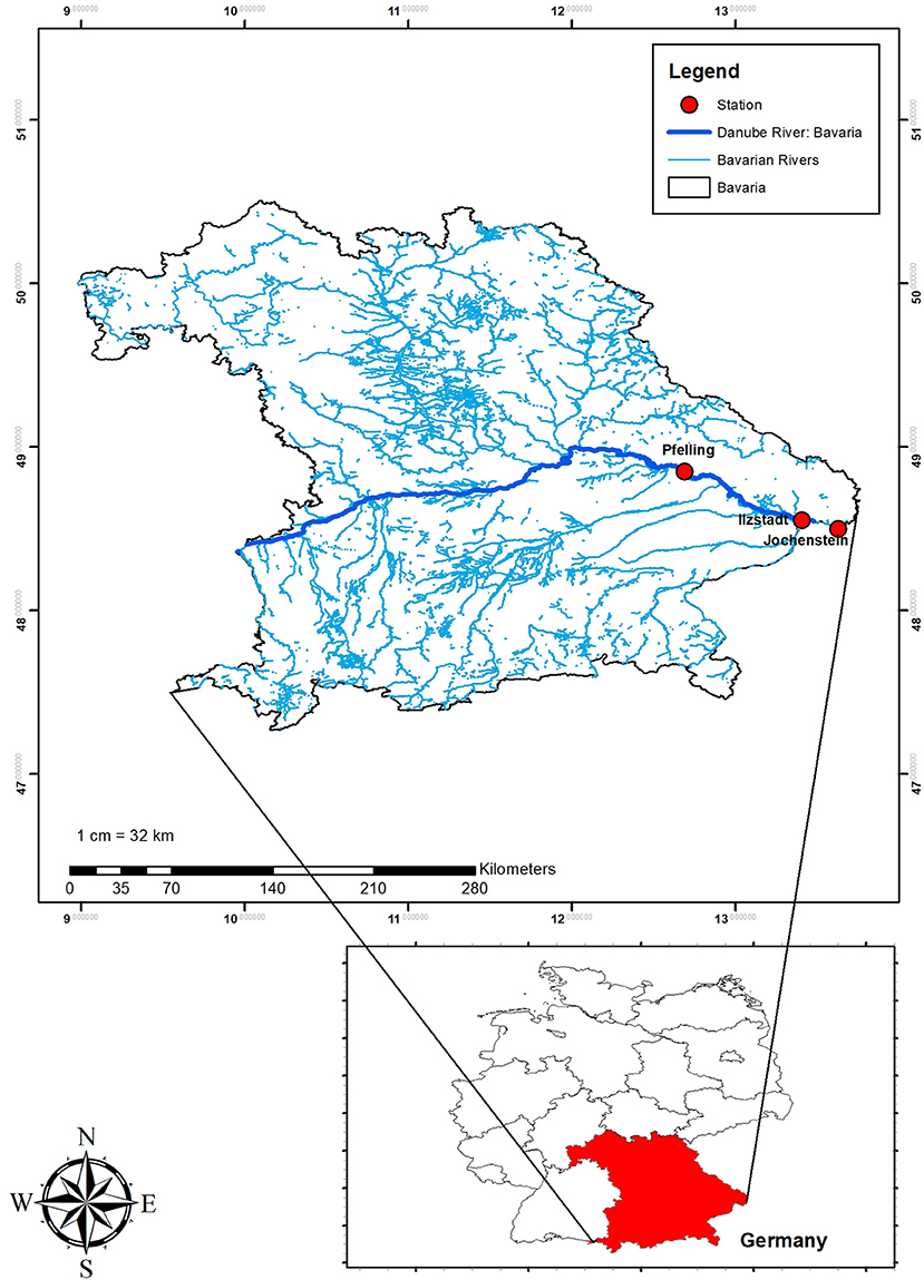
Figure 1. Locations of automatic measurement stations on Danube River.

Eight water quality constituents in each station including Dissolved Oxygen (DO), Temperature (Temp), Electronic Conductivity (EC), pH, Chlorophyll-a (Chl-a), Nitrate (${\text{NO}}_3^{-}$-N), orthophosphate (${\text{PO}}_4^{3-}$-P), and ammonium (${\text{NH}}_4^{+}$-N) are measured at both Pfelling and Jochenstein stations. Except for Chl-a concentration, which is measured hourly, the other physio-chemical parameters are measured at 15-minute intervals using in-situ automatic monitoring instruments. DO, Temp, EC, pH, and Chl-a were measured with a YSI multiparameter probe. Nutrients in two chosen stations are continuously measured with these three types of sensors. ${\text{NO}}_3^{-}$-N is recorded with an optical sensor because dissolved nitrate in water absorbs UV light with a wavelength below 250 nm. ${\text{NH}}_4^{+}$-N is measured with a gas ion-selective electrodes sensor. The available ammonium in the sample is converted into gaseous ammonia by adding a sodium hydroxide solution. Only the ${\text{NH}}_3^{+}$ gas passes the gas-permeable membrane of the electrode and is detected. A wet-chemical analyzer measures ${\text{PO}}_4^{3-}$-P in water. The color intensity is proportional to the ${\text{PO}}_4^{3-}$-P content of the sample in the specified measuring range. Samples that contain solids must be homogenized before entering the process photometer. The discharge data representing both stations are also available at 15-min intervals. The upstream discharge is measured at the same location of the Pfelling station, while the downstream discharges are taken from the closest discharge station, namely Ilzstadt (Figure 1).

Forty-five months of all data (from 01-03-2017 to 31-12-2020) for the Pfelling station and 57 months of all data (from 01-03-2016 to 31-12-2020) for the Jochenstein station are chosen to build the nutrient surrogate models, respectively. The raw data of temporal behavior of water quality constituents and nutrients are presented in Supplementary Figures 2–19.

Data analysis framework

All data analysis and model building use open-source libraries and frameworks of Python 3.8 useful for data analysis as Pandas (1.1.3), NumPy (1.19.2), blac (1.5.2), Scikit-learn (0.23.2). The specific functions are indicated later. The general overview of the workflow and procedures for building surrogate nutrient models presented in Figure 2.

FIGURE 2

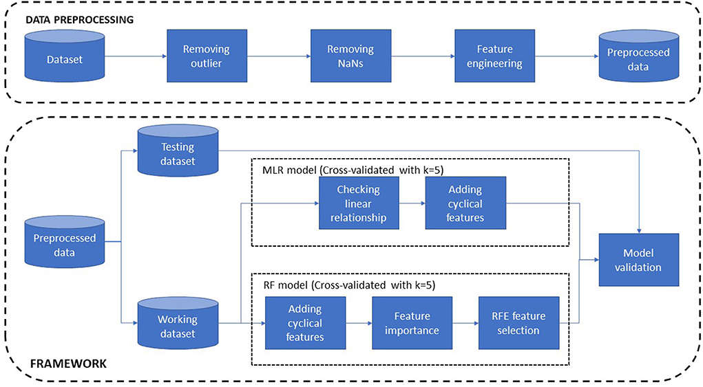
Figure 2. The overview of data preprocessing and framework.

Data pre-processing

Before starting data preprocessing, the percentage of non-detections in the raw data sets are first checked (Supplementary Table 2). Data cleaning is a crucial step because gaps or outliers can affect the model performance. To remove outliers, a moving mean filter is applied with a sliding window of 6 h (24 data points). If a value is more or less than three local standard deviations away from the local mean within the window, it will be defined as an outlier and removed. Maintenance or calibration procedures performed regularly at the stations can lead to data gaps. The timing and time spans of these interruptions varies from sensor to sensor. These gaps affect the implementation of the surrogate models, which cannot deal with not a number (NaN) values and therefore, an additional cleaning phase is required. NaN values in target variables and the corresponding values in predictors were removed. The rest of NaNs in predictors were filled by linear interpolation. A table that summarizes the statistics of water quality parameters and discharges after cleaning is given in Table 1.

TABLE 1

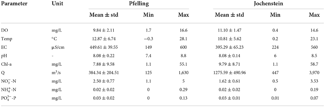
Table 1. Statistics of all water quality parameters in two stations.

As the multivariate linear regression (MLR) modeling assumes a normal distribution of variables (Uyanik and Güler, 2013), the normal distribution of both the target variables and predictors were tested using Probplot of Scipy library. As a result, Chl-a and Q were log-transformed because they have positive skews. The log transformation is the most popular among the different types of transformations used to transform skewed data to approximately conform to normality (Feng et al., 2014). After the pre-processing procedures, the available numbers of records and the percentages of total records for different nutrient models are shown in Table 2.

TABLE 2

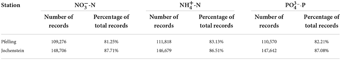
Table 2. Number of records and percentage of total records for different targets after cleaning.

Data partition

After the preprocessing procedures, the data is divided into working and test datasets using the train_test_split function in the Scikit-learn (0.23.2) library. The working subset is used to build the model, and the test subset evaluates the final model's performance as unseen data. Specifically, 80% of the dataset acts as working, and 20% of the dataset acts as testing. Further, the working subset was split into training and validation sets in each specific model during the building model process by applying k-fold cross-validation with k = 5. K-fold cross-validation generally results in a less biased or less optimistic estimate of the model skill. With this method, the working dataset is split into k fractions or folds, with each used iteratively as a validate set while the remaining k-1 fractions were used as a training set.

Predictor selection and optimization

Default input features, including DO, Temp, EC, pH, Q, and Chl-a, are feed to the models as predictors to simulate the nutrient concentrations (${\text{NO}}_3^{-}$-N, ${\text{NH}}_4^{+}$-N, and ${\text{PO}}_4^{3-}$-P) at each station in the Danube River. Hence, we developed cyclical features namely the month of a year, day of a month, and hour of a day as predictors. This technique is one of techniques in feature engineering. Feature engineering is the process of selecting, manipulating, and transforming raw data into features that can be used in supervised learning. In simple terms, it is the act of converting raw observations into desired features using statistical or machine learning approaches. The cyclical futures are represented as (x, y) coordinates on a circle, where the lowest value appears right next to the highest value (Supplementary Figure 1). This is performed using the inbuilt “sin” and “cos” functions in “NumPy.” In the end, there are 6 cyclical time features created as input predictors, namely month_sin, month_cos, day_sin, day_cos, hour_sin, and hour_cos. More details about the cyclic time features are described in SI. All the predictors, including both default features and the newly created cyclical features, were applied for linear models and RF models.

Multiple linear regression models

Multiple Linear Regression (MLR) is used in this work as the linear relationship between the predictors and targets is expected. The Multiple Linear Regression (MLR) is expressed as equation below:

$\begin{array}{cc}\widehat{\text{y}}={\text{b}}_0+{\text{b}}_1{\text{X}}_1+{\text{b}}_2{\text{X}}_2+\dots +{\text{b}}_{\text{p}}{\text{X}}_{\text{p}}& (1)\end{array}$

where ŷ indicator is the predicted or expected value of the dependent variable, X₁ through X_p are p distinct independent or predictor variables, b₀ is the value of y when all of the independent variables (X₁ through X_p) are equal to zero, and b₁ through b_p are the estimated regression coefficients.

The linear relationship between predictors and target variables is checked by computing the standard correlation coefficient by the corr() function in Pandas library. By default, the function calculates Pearson Correlation coefficient, using the equation:

$\begin{array}{cc}r=\frac{{\displaystyle \sum (x_i-\overline{x})(y_i-\overline{y})}}{\sqrt{{{\displaystyle \sum }(x_i-\overline{x})}^2{{\displaystyle \sum }(y_i-\overline{y})}^2}}& (2)\end{array}$

where i represents each observation, x is a predictor and $\overline{x}$ is its mean value, and y is a target variable with $\overline{y}$ being its mean value.

This approach may be used to determine the relationship between predictors and targets in a dataset. The order of default input features added to the linear model depends on the degree of the correlation between the predictor and target. The linear model is implemented to fit from one to six predictors, and the performance is evaluated, respectively. After the six predictors, cyclical time features are also added to the model to test if it could improve the performance.

Random forest models

RF is applied to build the nutrient surrogate models in this work. To have a comparison of linear models, the order of default input variables added to the RF models is exactly the same as the order in linear models. In order to find out the ideal set of hyperparameters, the model is run with a grid of default hyperparameter values. Function GridSearchCV of Scikit-learn library is used to perform this process, using the cross-validation k = 5 and 10 trees. The predefined grid is presented in Table 3. This setting produces 54 candidates, multiplied by five-folds, totaling 270 fits. The best-fitting hyperparameters are used in the models is presented in Supplementary Table 1. Finally, the model is tested with the unseen data.

TABLE 3

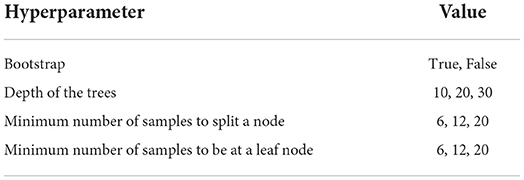
Table 3. Values of the hyperparameters contained in the grid search.

Feature selection refers to techniques that select a subset of the most relevant features for a dataset. Fewer features can allow machine learning algorithms to run more efficiently (less space or time complexity) and be more effective. Some machine learning algorithms can be misled by irrelevant input features, resulting in worse predictive performance. Recursive Feature Elimination (RFE) is a wrapper-based feature-ranking technique that uses optimization algorithms to explore inside the input space for the best subset. This method was used for only RF models, to test if it could improve the performance of the models with the minimum number of predictors. RFE works by searching for a subset of features by starting with all features in the training dataset and successfully removing features until the desired number remains. In each iteration, one variable is deleted based on the Root Mean Square Error (RMSE) values, and a new RF model is developed with the remaining variables. This method is repeated until only one variable was left as the input feature. Five-fold cross-validation is used to optimize predictor selection throughout the elimination phase. The model with the lowest RMSE is chosen as the best model during the recursion process; if another model with a different collection of variables is discovered, it is automatically updated and ranked. Finally, it selects the optimized subset of the predictors that provide the least RMSE. This is achieved by fitting the given machine learning algorithm used in the core of the model, ranking features by importance, discarding the least important features, and re-fitting the model (Granitto et al., 2006). RF is a decision-tree model, which can compute the feature importance score with the built-in attribute.

The overview of data preprocessing and framework is demonstrated in Figure 2.

Model evaluation and performance comparison

The coefficient of determination (R²), the Root Mean Square Error (RMSE) and normalized RMSE (nRMSE) are used to evaluate the performance of models. The RMSE calculates the variance of errors regardless of sample size and shows the difference between actual and predicted values. As a result, the RMSE of a perfect match between observed and projected values would be 0 (Barzegar et al., 2018). The RMSE equation is as below:

$\begin{array}{cc}RMSE=\sqrt{\frac{{\displaystyle {\sum }_{i=1}^N}{(y_i-\widehat{y_i})}^2}{N}}& (3)\end{array}$

where y is the observed value, ŷ is the predicted value, and N is the number of observations.

nRMSE is calculated by dividing RMSE by the mean of data. Using nRMSE for comparing the performances among different nutrient variables is helpful because they have different scales.

R² is also computed to evaluate the performance of models.

$\begin{array}{cc}{R}^2=1-{\displaystyle \sum \frac{{(y_i-{ŷ}_i)}^2}{{(y_i-\overline{y})}^2}}& (4)\end{array}$

The performances of the final RF models and the MLR models with the unseen data (test dataset) are computed and compared using the abovementioned statistics.

Results

Correlation between targets and variable predictors

A first insight of the relationship between the predictors and the target variables was conducted by means of the Pearson's coefficient. Results are summarized in Table 4. Overall, the correlation between targets and predictors in Jochenstein is higher than in Pfelling station and some variables are reporting significant low correlation, with absolute r-values lower than 0.01.

TABLE 4

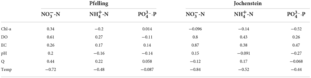
Table 4. Pearson's r for each of the target variables concerning the six predictors.

For example, in Pfelling station, ${\text{NO}}_3^{-}$-N displays a strong linear relationship with Temp (r = −0.72) and DO (r = 0.61). Although EC in Pfelling station does not strongly correlate with ${\text{NO}}_3^{-}$-N, EC in Jochenstein station got the highest r = 0.87 in the relationship with ${\text{NO}}_3^{-}$-N. Temp and DO also occur in strong relationship with r = −0.84 and 0.8, respectively. Considering ${\text{NH}}_4^{+}$-N as target, the Pearson's coefficient reveals a strong linear relationship with Temp (r = −0.48) and DO (r = 0.27). Similarly, Temp and DO also strongly correlate with ${\text{NH}}_4^{+}$-N in Jochenstein station, with r = 0.52 and −0.43, respectively. The seasonal behavior of nutrients explains the strong relationship between nutrients concentrations and Temp. The solubility of nutrients increases in summer and autumn, coinciding with high-temperature periods and decreases with low-temperature periods. ${\text{PO}}_4^{3-}$-P in Pfelling station does not present a strong relationship with any variables. The highest correlation coefficients are 0.14 for EC and −0.14 for pH. Compared with ${\text{PO}}_4^{3-}$-P in Pfelling station, ${\text{PO}}_4^{3-}$-P in Jochenstein station has a better correlation with predictors, with Chl-a (r = −0.52) having the strongest correlation.

Model performance with surrogate variables and cyclical features

The strength of the correlation was chosen as the determining criteria to select the order in which the variables feed the models. Table 5 shows details of the input variables and the order in which they were selected. Additionally, no further regularization was used because the models fitted on training data performed similarly to those fitted on validate data. This is due to a large number of observations compared to the number of predictors. Overall, the performance of linear models for both stations to predict ${\text{NO}}_3^{-}$-N is higher than the prediction of ${\text{NH}}_4^{+}$-N and ${\text{PO}}_4^{3-}$-P. In linear models of ${\text{NO}}_3^{-}$-N, an R² higher than 0.50 was achieved using just one predictor and continued improving until six predictors were used, achieving 0.62 and 0.87 for Pfelling and Jochenstein, respectively. In contrast, the linear model of ${\text{PO}}_4^{3-}$-P in Pfelling station got R² = 0 when adding only one feature, which means the model cannot retrieve any information if there is only EC as a predictor. When adding more predictors, R²-value kept increasing and achieved the highest value of 0.22. The linear model of ${\text{PO}}_4^{3-}$-P in Jochenstein station got better performance, which is R² = 0.48 when all default surrogate variables were added. Regarding linear models of ${\text{NH}}_4^{+}$-N, they achieved R² = 0.33 and 0.40 for Pfelling station and Jochenstein station, respectively. In general, linear models of nutrients in Jochenstein station have better performance than linear models in Pfelling station.

TABLE 5

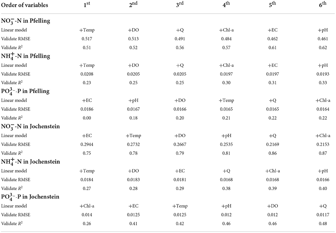
Table 5. Validation RMSE for each target variable and each subset of variables of size one to six in the MLR model.

The percentage of reduction in RMSE when adding more variables in the MLR model and RF model is shown in Figure 3. When all six predictors were added, the reduction of RMSE compared to using only one predictor in RF varies from 49.60 to 75.95%, while MLR varies from 7.21 to 26.87%. RF models improved their performances in surrogating nutrients more significantly, including more predictors than MLR. Significantly, RF models have higher improvement than MLR models with only two predictors. When adding three or more variables, RF outperforms MLR significantly. In contrast to linear models, which are unable to leverage most of the information that can be obtained using inexpensive and widely accessible sensors, RF proves to be very efficient and effective in using the available information, highlighting their applicability to describe environmental phenomena. Then, the gradient of the RMSE reduction decreases shows that adding more variables will not improve the performance of models considerably. For Pfelling station, the RF models with more than four variables did not improve RMSE by more than 5%. For the Jochenstein station, with more than five predictors, the RF models did not obtain any RMSE improvements higher than 5%.

FIGURE 3

Figure 3. Percentage of reduction of test RMSE as a function of the number of predictors in MLR and RF models in (A) Pfelling station and (B) Jochenstein station.

Additionally, adding time features as additional predictors has a significant impact on the model and error metrics' performances. The percentages of reduction in RMSE in the MLR and RF models when adding time features are presented in Table 6. The models with all surrogate variables are chosen as benchmarked. From the computed results, RF models obtain a considerable benefit from cyclical features. Although MLR models also have some improvements, they are not significant as RF. When adding time features to MLR models, the performance improved from 0.6 to 10.78%, while RF models improved from 7.69 to 20.51%. ${\text{NO}}_3^{-}$-N in Pfelling station received the most influence from cyclical features for both types of models, in both stations. The performance of RF models for predicting ${\text{NO}}_3^{-}$-N achieved a RMSE reduction of 20.51% for Pfelling station and 15.13% for Jochenstein station. The performance of RF models of ${\text{NH}}_4^{+}$-N and ${\text{PO}}_4^{3-}$-P also improved, with 18.07 and 13.16% for Pfelling station, and 7.69 and 11.11% for Jochenstein station, respectively.

TABLE 6

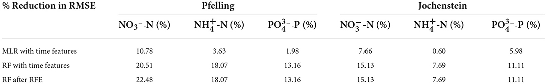
Table 6. Percentage of reduction in validate RMSE in linear models and non-linear models with time features and RFE.

Feature importance and optimal predictors

Feature evaluation based on the Feature Importance attribute of Random Forest was also applied. Results from this evaluation are shown in Figure 4. Note that the importance of input predictors is different for each retrieved target. For retrieving ${\text{NO}}_3^{-}$-N and ${\text{NH}}_4^{+}$-N, Temp is the most contributing factor for both stations. Chl-a also plays a vital role in simulating nutrients in rivers, especially with ${\text{NH}}_4^{+}$-N and ${\text{PO}}_4^{3-}$-P. In addition, EC also exhibits relevant importance in predicting nutrients in those stations. Besides, the created cyclical time features also contribute significantly to the simulation of nutrients, especially the month features. For example, the month_cos feature contributed most significantly to predicting ${\text{PO}}_4^{3-}$-P of Jochenstein station. For retrieving ${\text{NO}}_3^{-}$-N in both stations, month_sin also contributed notably. The feature selection results show that month data plays a vital role in the model, which could support the model to study the seasonality of targets. The relative importance of predictors does not match with the correlation strength rankings. Chl-a in Pfelling station, for example, has the weakest linear relationship with ${\text{PO}}_4^{3-}$-P, but it is the most contributing feature in RF model for predicting ${\text{PO}}_4^{3-}$-P. DO has strong correlation with ${\text{NO}}_3^{-}$-N in both stations, but this feature did not contribute significantly to the performance of RF models. These results show that the correlation between predictors and targets cannot decide the relative importance in the non-linear models.

FIGURE 4

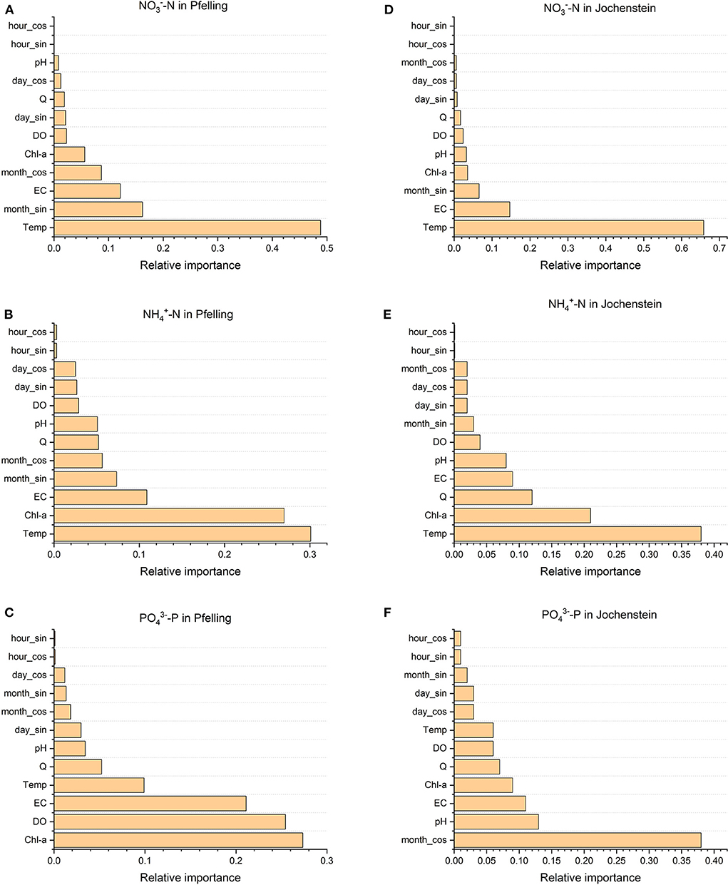
Figure 4. Feature importances in RF models of different nutrients in Pfelling and Jochenstein station. (A) ${\text{NO}}_3^{-}$-N Pfelling. (B) ${\text{NH}}_4^{+}$-N Pfelling. (C) ${\text{PO}}_4^{3-}$-P Pfelling. (D) ${\text{NO}}_3^{-}$-N Jochenstein. (E) ${\text{NH}}_4^{+}$-N Jochenstein. (F) ${\text{PO}}_4^{3-}$-P Jochenstein.

The performance of RF models after optimizing feature inputs by the RFE method is shown in Table 6. Initially, all RF models have 12 predictors, including default variables and time features. After implementing RFE, although the model performances do not improve significantly, the numbers of the predictors used in the models are largely reduced. Table 7 presents the list of optimized predictor subsets after applying RFE with five-fold cross-validation. Five out of six targets require all the default surrogate variables combined with newly created cyclical time features to give out the best performance. The only exception is ${\text{NO}}_3^{-}$-N in Pfelling station, which requires only four surrogates (DO, Temp, EC, and Chl-a) and 2 cyclical month-in-a-year features. The RF model of ${\text{NO}}_3^{-}$-N in Jochenstein station need 8 features. For retrieving ${\text{NH}}_4^{+}$-N, RF models require 8 and 12 features for Pfelling station and Jochenstein station, respectively. The RF models of ${\text{PO}}_4^{3-}$-P demand the highest number of predictors in both stations, with 10 predictors for Pfelling station and 12 predictors for Jochenstein station. Generally, at least two cyclical features are needed in the models to give out the least error results. After applying RFE, all the month features are left, corresponding to the findings of feature importance. It can be concluded that implementing RFE can support in finding the best subsets of predictors with similar good performance when using all predictors.

TABLE 7

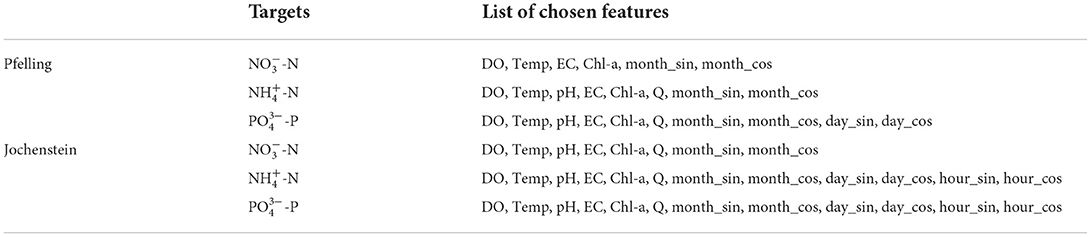
Table 7. List of chosen variables.

Evaluation on unseen data

To finally test the algorithms on unseen data, the best MLR and RF models with better RMSE, nRMSE, and R² are chosen as the final surrogate models. Calibration is done accordingly with the test dataset that produced best error metrics. Results are shown in Table 8.

TABLE 8

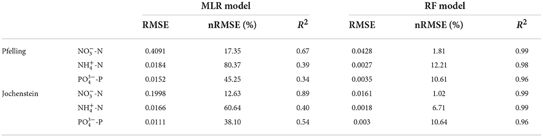
Table 8. Performance on testing dataset.

In general, the performance of MLR and RF models on unseen data is similar to the working datasets. According to these results, the RF models can reproduce the data trend, data seasonality and present a reliable estimation of ${\text{NO}}_3^{-}$-N, ${\text{NH}}_4^{+}$-N, and ${\text{PO}}_4^{3-}$-P concentrations. Performance on unseen dataset reproduce water quality trends with high-accuracy prediction capacity for ${\text{NO}}_3^{-}$-N (R² = 0.99), ${\text{NH}}_4^{+}$-N (R² = 0.98 and 0.99), ${\text{PO}}_4^{3-}$-P (R² = 0.96). Based on this, all RF models, including feature engineering, feature selection, and hyperparameter tuning, outperformed MLR models. The decreases in RMSE values of RF models in nutrient simulations compared with the MLR models range from 73% (${\text{PO}}_4^{3-}$-P in Jochenstein station) to 92% (${\text{NO}}_3^{-}$-N in Jochenstein station). In Pfelling station, RF models improved the RMSE compared to MLR performance of simulating ${\text{NO}}_3^{-}$-N from 0.4091 to 0.0428, ${\text{NH}}_4^{+}$-N from 0.0184 to 0.0027, ${\text{PO}}_4^{3-}$-P from 0.0152 to 0.0035. The improvement in RMSE between RF and MLR models in Jochenstein station is from 0.1998 to 0.0161 for ${\text{NO}}_3^{-}$-N, from 0.0166 to 0.0018 for ${\text{NH}}_4^{+}$-N, and from 0.0111 to 0.003 for ${\text{PO}}_4^{3-}$-P.

In general, the RF models can reproduce the water patterns with higher accuracy than MLR models as seen in Figure 5, which displays the first 100 simulation results for both models together with field data, particularly at peak values of targets. However, this behavior is not stably. For examples, in the prediction of ${\text{NH}}_4^{+}$-N and ${\text{PO}}_4^{3-}$-P in Jochenstein station, some peak observed values cannot be simulated by RF models. On the other hand, the MLR algorithm even simulates some negative values (${\text{NH}}_4^{+}$-N and ${\text{PO}}_4^{3-}$-P), which is unrealistic.

FIGURE 5

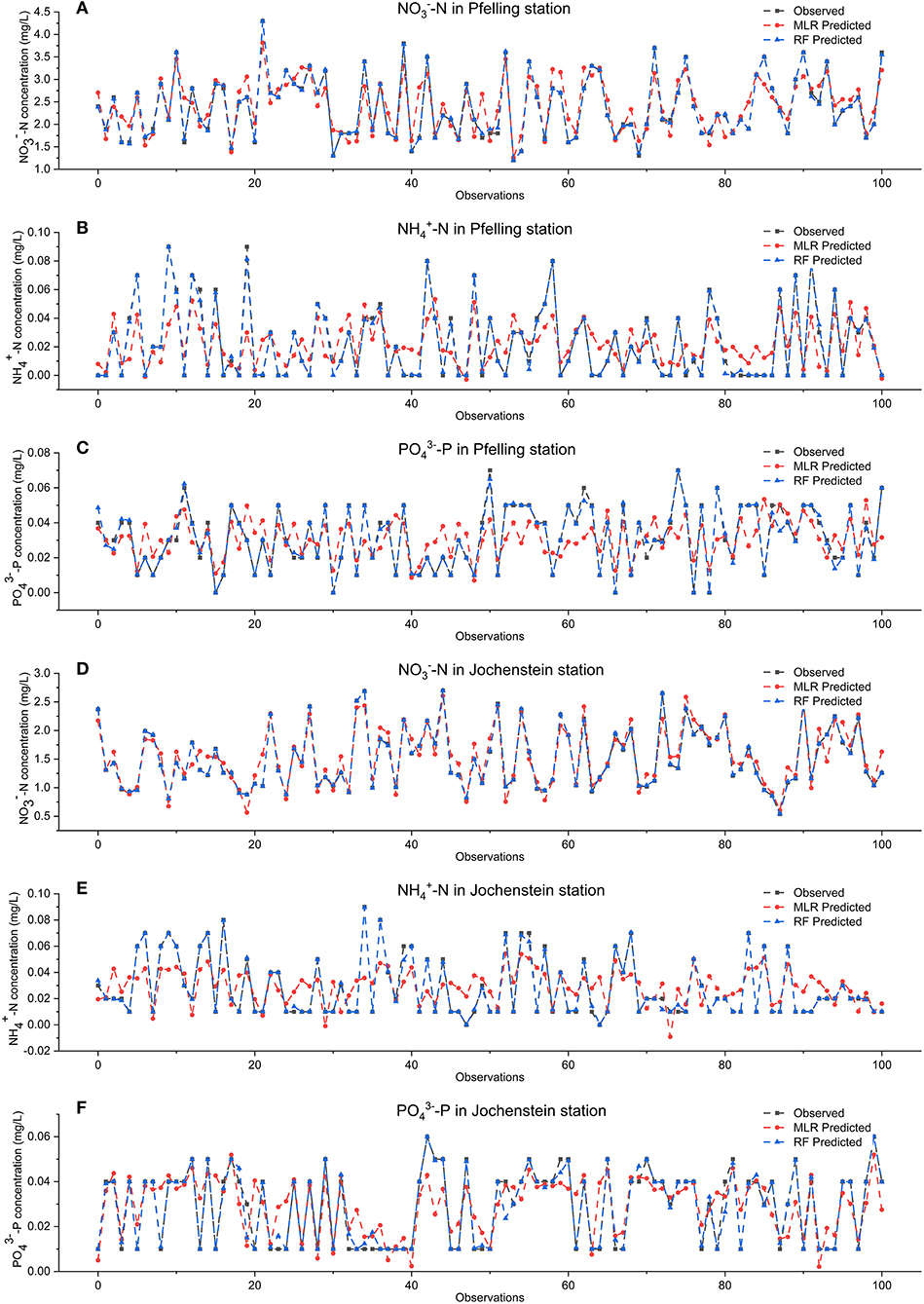
Figure 5. Observed and predicted values for the first 100 observations of the testing dataset in Pfelling and Jochenstein station. (A) ${\text{NO}}_3^{-}$-N Pfelling. (B) ${\text{NH}}_4^{+}$-N Pfelling. (C) ${\text{PO}}_4^{3-}$-P Pfelling. (D) ${\text{NO}}_3^{-}$-N Jochenstein. (E) ${\text{NH}}_4^{+}$-N Jochenstein. (F) ${\text{PO}}_4^{3-}$-P Jochenstein.

Discussion

The strong correlations for MLR models of ${\text{NO}}_3^{-}$-N achieved R² on unseen data of 0.67 for Pfelling station and 0.89 for Jochenstein station. In contrast, ${\text{NH}}_4^{+}$-N and ${\text{PO}}_4^{3-}$-P have lower correlations with the predictors, which leads to the low performances of their MLR models. Linear models are unable to leverage most of the information that can be obtained using inexpensive and widely accessible sensors when there is a strong linear correlation. The performances of ${\text{NH}}_4^{+}$-N and ${\text{PO}}_4^{3-}$-P simulations after using RF have improved more significantly than those of ${\text{NO}}_3^{-}$-N. The different performances between MLR models and RF models proved that the RF models are more efficient and effective in using the available information, especially if the correlations between the target nutrient and predictors are not strong. The capability of using RF to leverage the model performance is more pronounced if there is no strong linear correlation. Our results highlight the applicability and capability of RF models to describe the relationship between nutrients and other water quality constituents, which, as many other environmental phenomena, are often non-linear. In this study, in addition to the robust capability of RF models in dealing with non-linear relationships, the outperformance of RF can also benefit from the large amount of input data, including the use of different available sensors as predictors, as well as massive records of observations for model building and training. Both aspects facilitate RF models in learning and understanding data behavior.

There are many previous studies applying linear regression models as a surrogate for water quality constituents of particular interest. For example, Lessels and Bishop (2013) got R² ranging from 0.28 to 0.45 in predicting the total phosphorus concentrations for sub-catchments within the greater Lake Buragorang catchment in Australia; Olli and Song (2006) got R² from −16.64 to 0.95 for predicting the Chl-a concentration in Finnish lakes; Jones et al. (2004) achieved R² varying from 0.62 to 0.76 in the regressions for total phosphorus and total nitrogen concentrations of Missouri reservoirs. The MLR models which are used in this work obtained R² varies from 0.34 to 0.89. These results indicated that the MLR models could retrieve nutrient concentration, but with limited accuracy. Recent studies have applied various ML algorithms in retrieving water quality surrogate models, which obtained good performances. For example, García Nieto et al. (2019) applied the Support Vector Machine method for total phosphorus by using biological and physio-chemical variables in 2006–2014 and achieved R² of 0.9; Chen and Liu (2015) applied adaptive neuro-fuzzy inference system for retrieving total phosphorus in 1993–2003 and obtained R² of 0.86; Kim et al. (2012) applied ANN for hydro-meteorological dataset in 1994–2000 and obtained R² of 0.99; Ha et al. (2020) applied RF for water quality dataset 2009-2014 and received R² in the range 0.88–0.90; RF was used in Castrillo and García (2020) and Shen et al. (2020), but there was no reported R². Generally, the R²-values of RF models in this study are higher than MLR models, which is in line with previous studies. This indicates that using non-linear regression methods is more powerful in water quality surrogate models. Furthermore, the performance of RF models in this work is higher than in previous studies. This result proves that the model development methods which are proposed improve the performance of RF models significantly.

One of the highlights of this study is the framework, including intermediate steps of creating time series data as cyclical features and finding the best subset of predictors by RFE. In this work, the time-series data are encoded to cyclical features, which support the models to study the seasonality of targets in water, and the RFE method is applied to find out the most relevant subsets which give out the least error performance. According to Table 6, ${\text{NO}}_3^{-}$-N models for both stations, obtained the most significant benefit from including cyclical time features compared with the models for other nutrients. Weilguni et al. (2000) has examined 39-year of data (1957–1995) of different water quality parameters in the Danube River and discovered that seasonal patterns were most pronounced for nitrate, slightly less for total phosphorus, soluble reactive phosphorus, and ammonium. This explains why RF models of ${\text{NO}}_3^{-}$-N receive the most benefits with time series features. Relative importance results also show that the 2 month-in-a-year features (namely month_sin and month_cos) contributed significantly to the performance of all RF models.

Comparing the performance of RF models without and with RFE method, the performance does not improve significantly. These findings are similar to the study by Chakraborty and Elzarka (2019). They have determined that including an external feature selection algorithm for a tree-based model brings hardly any difference in model performances. However, the best performance could be achieved with fewer predictors thanks to RFE method, which is the purpose of implementing RFE in this model. The RFE provides a helpful tool for optimizing a cost-effective soft sensor in water management. In comparison between Figure 4 and Table 7, it is evident that the predictors which have low relative importance have been removed after implementing RFE. Relative importance tell which predictors are most influential in RF models, and RFE optimizes the models by giving out the best subset of predictors with the minor error. Furthermore, the difference between Figure 4 and Table 4 indicates that the relative importance of predictors does not match the linear correlation. For example, in the case of ${\text{PO}}_4^{3-}$-P in Pfelling station, Chl-a has the weakest correlation with the target but contributes the most significantly to the performance of RF model. This shows that in order to reduce the sensor numbers and design cost-effective surrogate models with RF, relative importance should be implemented. It cannot be replaceable by conducting the linear correlation analysis because the relationship between the predictors and the targets is non-linear. In addition, the presence of covariance between the various variables has practical implications that must be considered throughout the soft-sensor design process. When a group of surrogate sensors includes a primary sensor that offers the most information and multiple non-covariant sensors, a lot of information may be obtained with only a few sensors. Our study shows that intermediate steps (feature engineering + relative importance + RFE) are essential in designing a cost-effective soft-sensor system. The relative importance of predictors would allow the water managers or other stakeholders to make a cost-benefit analysis in the decision-making of the installation of sensors.

One of ten problems regarding the practical implementation of the Water Frame Directive that has been recognized is inconsistent and inadequate monitoring frequently results in a lack of knowledge of relevant chemicals and peak concentrations, resulting in undiscovered dangers (Brack et al., 2017). Applying modeling have been recommended as a tool to fill in gaps in monitoring data and generate incentives to expand the chemical pollution monitoring base across Europe. Many chemicals, such as key nutrients [nitrogen (N) and phosphorus (P)], are now mostly monitored by analytical discrete campaigns with low sample frequency. The RF algorithm, which has been demonstrated in this work, has proved its ability in studying the underlying relationship between predictors and targets, resulting in a reliable prediction of high-frequency nutrient concentrations in the Danube River. The output of the models, the computed real-time high-frequency nutrient concentrations, may be used directly or fed into process-based water quality models to enhance understandings in nutrient processing (Huang et al., 2022) and eutrophication forecasting while reducing the cost and time effectiveness of traditional sampling approaches. Besides, the soft-sensors can increase the data availability as well as overcome the period when the data from in-situ sensors is unavailable due to reasons such as calibration, maintenance, drifting, failure, etc.

Although ML has been successful in the water management sector, there are still some perceptions that ML models are “black boxes,” meaning the ML method is thought to take inputs and provide outputs but not yield interpretable information to the user. In addition, the discrepancies of the results among the datasets underlined how this kind of black-box regressor could have strongly site-specific validity. A regression model between the response and explanatory factors is usually site-specific, and it may vary over time if the constituent's sources change or if a better sensor becomes available. Turbidity measurements, for example, are influenced by the size, color, and density of suspended-sediment particles (Ziegler, 2003; Anderson, 2005). Therefore, regression analysis is site-specific, and the regression model must be checked and updated on an annual basis through continuing data collection. The results of this study also confirm the site-specific characteristic of regression model. Although the two chosen stations are on the same river, the relative importance of predictors is different. Furthermore, this work could be additionally developed by collecting a larger dataset with data coming from a higher number of measurement stations on the river, which could more robustly substantiate general conclusions on the cause-effect relationship describing the phenomena.

This study proposes an innovative soft sensor based on RF regression models for real-time virtual monitoring of nutrient concentration on the Danube River. Relying on data from two automatic measurement stations, soft-sensor regressors used different physical and chemical characteristics as predictors and gave satisfying performances. Performances of the RF model were significantly higher and more stable than the MLR model, highlighting the importance of non-linearities and interactions in the relationships between water qualities and nutrient concentration in the river. The findings demonstrate the presence of useful data that may be utilized to acquire derived data at a reasonable cost. It is noteworthy to emphasize the rising relevance of incorporating current open data services into models, which may be included into the models thanks to the development of ubiquitous and economical network connections, offering additional data sources at almost no cost. This benefits both the academic community and society since it encourages collaboration, reduces the expense of redundant studies, and enhances transparency, among other benefits. In addition, the regression models can be uploaded into underlying website software, that computes the concentrations of target variables and generates plots and data tables, which are open-accessed for assessing the feasibility of the models. Furthermore, similar studies for the future should be conducted to verify the applicable of the proposed framework.

Conclusions

In this work, RF algorithm could reproduce the environmental phenomena, especially nutrient dynamics in high frequency, present in the water quality dynamics and contribute to water quality management. Additionally, RF has the ability to simulate the peak values of concentration in nutrients, in contrast with MLR model which even predicts some negative values. By combining with encoding time-series data and feature selection, the performance of RF models has been improved. Additionally, because of the complicated relationships underneath machine learning models, the variable selection process cannot be considered as an independent procedure to be carried out without regard to which model to be used. This work provides a description of the methodology, including intermediate steps (time series as cyclical features, RFE, feature importance) used to train and validate the water quality models and highlights that machine learning approaches and the RF in particular can represent the complex environmental phenomena, making them a promising water quality management technique.

Data availability statement

Publicly available datasets were analyzed in this study. This data can be found here: https://www.gkd.bayern.de/. The python code is provided at https://github.com/yentran0402/nutrients-soft-sensor.

Author contributions

JH persuade the presented idea. YT and LA-R developed the methodology. YT initiated first manuscript draft. All authors have made a substantial, direct, and intellectual contribution to the work and approved it for publication.

Funding

We appreciate the support from the Open Access Publishing Fund of the Technical University of Munich (TUM).

Acknowledgments

We would like to acknowledge the assistance of the following individuals: Ludwig Butz from Water Management Authority Deggendorf, the station operators at Pfelling and Jochenstein station for providing essential information; We would also like to thank An Tran and Pham Thoai for consulting and discussions regarding model development.

Conflict of interest

The authors declare that the research was conducted in the absence of any commercial or financial relationships that could be construed as a potential conflict of interest.

Publisher's note

All claims expressed in this article are solely those of the authors and do not necessarily represent those of their affiliated organizations, or those of the publisher, the editors and the reviewers. Any product that may be evaluated in this article, or claim that may be made by its manufacturer, is not guaranteed or endorsed by the publisher.

Supplementary material

The Supplementary Material for this article can be found online at: https://www.frontiersin.org/articles/10.3389/frwa.2022.894548/full#supplementary-material

References

Anderson, C. W. (2005). Turbidity (ver. 2.1): U.S. Geological Survey Techniques of Water-Resources Investigations.

Barzegar, R., Asghari Moghaddam, A., Adamowski, J., and Ozga-Zielinski, B. (2018). Multi-step water quality forecasting using a boosting ensemble multi-wavelet extreme learning machine model. Stochastic Environ. Res. Risk Assess. 32, 799–813. doi: 10.1007/s00477-017-1394-z

CrossRef Full Text | Google Scholar

Belgiu, M., and Qăgut, L. (2016). Random forest in remote sensing: a review of applications and future directions. ISPRS J. Photogramm. Remote Sens. 114, 24–31. doi: 10.1016/j.isprsjprs.2016.01.011

CrossRef Full Text | Google Scholar

Brack, W., Dulio, V., Ågerstrand, M., Allan, I., Altenburger, R., Brinkmann, M., et al. (2017). Towards the review of the European Union Water Framework Directive: recommendations for more efficient assessment and management of chemical contamination in European surface water resources. Sci. Tot. Environ. 576, 720–737. doi: 10.1016/j.scitotenv.2016.10.104

PubMed Abstract | CrossRef Full Text | Google Scholar

Breiman, L. (2001). Random Forests. Mach. Learn. 45, 5–32. doi: 10.1023/A:1010933404324

CrossRef Full Text | Google Scholar

Cai, Y., Guan, K., Peng, J., Wang, S., Seifert, C., Wardlow, B., et al. (2018). A high-performance and in-season classification system of field-level crop types using time-series Landsat data and a machine learning approach. Remote Sens. Environ. 210, 35–47. doi: 10.1016/j.rse.2018.02.045

CrossRef Full Text | Google Scholar

Cankurt, S., and Subasi, A. (2015). Developing tourism demand forecasting models using machine learning techniques with trend, seasonal, and cyclic components. Balkan J. Electric. Comput. Eng. 3, 42–49. Available online at: https://dergipark.org.tr/en/pub/bajece/issue/3357/46412

Google Scholar

Castrillo, M., and García, Á. L. (2020). Estimation of high frequency nutrient concentrations from water quality surrogates using machine learning methods. Water Res. 172, 115490. doi: 10.1016/j.watres.2020.115490

PubMed Abstract | CrossRef Full Text | Google Scholar

Chakraborty, D., and Elzarka, H. (2019). Advanced machine learning techniques for building performance simulation: a comparative analysis. J. Build. Perform. Simul. 12, 193–207. doi: 10.1080/19401493.2018.1498538

CrossRef Full Text | Google Scholar

Chen, W.-B., and Liu, W.-C. (2015). Water quality modeling in reservoirs using multivariate linear regression and two neural network models. Adv. Artif. Neural Syst. 2015, 1–12. doi: 10.1155/2015/521721

CrossRef Full Text | Google Scholar

Chou, J.-S., and Tran, D.-S. (2018). Forecasting energy consumption time series using machine learning techniques based on usage patterns of residential householders. Energy 165, 709–726. doi: 10.1016/j.energy.2018.09.144

CrossRef Full Text | Google Scholar

Corominas, L.l., Garrido-Baserba, M., Villez, K., Olsson, G., Cortés, U., and Poch, M. (2018). Transforming data into knowledge for improved wastewater treatment operation: a critical review of techniques. Environ. Modell. Softw. 106, 89–103. doi: 10.1016/j.envsoft.2017.11.023

CrossRef Full Text | Google Scholar

Costello, Z., and Martin, H. G. (2018). A machine learning approach to predict metabolic pathway dynamics from time-series multiomics data. NPJ Syst. Biol. Appl. 4, 19. doi: 10.1038/s41540-018-0054-3

PubMed Abstract | CrossRef Full Text | Google Scholar

Fawagreh, K., Gaber, M. M., and Elyan, E. (2014). Random forests: from early developments to recent advancements. Syst. Sci. Control Eng. 2, 602–609. doi: 10.1080/21642583.2014.956265

CrossRef Full Text | Google Scholar

Feng, C., Wang, H., Lu, N., Chen, T., He, H., Lu, Y., et al. (2014). Log-transformation and its implications for data analysis. Shanghai Arch. Psychiatry 26, 105–109. doi: 10.3969/j.issn.1002-0829.2014.02.009

PubMed Abstract | CrossRef Full Text | Google Scholar

Francke, T., López-Tarazón, J. A., and Schröder, B. (2008). Estimation of suspended sediment concentration and yield using linear models, random forests and quantile regression forests. Hydrol. Process. 22, 4892–4904. doi: 10.1002/hyp.7110

CrossRef Full Text | Google Scholar

García Nieto, P. J., García-Gonzalo, E., Fernández, J. R. A., and Muñiz, C. D. (2019). Water eutrophication assessment relied on various machine learning techniques: A case study in the Englishmen Lake (Northern Spain). Ecol. Modell. 404, 91–102. doi: 10.1016/j.ecolmodel.2019.03.009

CrossRef Full Text | Google Scholar

Granitto, P. M., Furlanello, C., Biasioli, F., and Gasperi, F. (2006). Recursive feature elimination with random forest for PTR-MS analysis of agroindustrial products. Chemometr. Intell. Lab. Syst. 83, 83–90. doi: 10.1016/j.chemolab.2006.01.007

CrossRef Full Text | Google Scholar

Guha, R., and Ng, S. (2019). A Machine Learning Analysis of Seasonal and Cyclical Sales in Weekly Scanner Data. National Bureau of Economic Research. doi: 10.3386/w25899

CrossRef Full Text | Google Scholar

Ha, N.-T., Nguyen, H. Q., Truong, N. C. Q., Le, T. L., Van Thai, N., and Pham, T. L. (2020). Estimation of nitrogen and phosphorus concentrations from water quality surrogates using machine learning in the Tri An Reservoir, Vietnam. Environ. Monitor. Assess. 192, 789. doi: 10.1007/s10661-020-08731-2

PubMed Abstract | CrossRef Full Text | Google Scholar

Harrison, J. W., Mark, A. L., Jeremy, L. F., Lawrence, W. E., and Rick, A. R. (2021). Prediction of stream nitrogen and phosphorus concentrations from high-frequency sensors using Random Forests Regression. Sci. Tot. Environ. 763, 143005. doi: 10.1016/j.scitotenv.2020.143005

PubMed Abstract | CrossRef Full Text | Google Scholar

Helsel, D. R., and Hirsch, R. M. (2002). Statistical Methods in Water Resources. Version 1.1. With Assistance of U.S. Geological Survey. Reston, VA (Techniques of Water-Resources Investigations, 04-A3). Available online at: http://pubs.er.usgs.gov/publication/twri04A3

Google Scholar

Hensley, R. T., Kirk, L., Spangler, M., Gooseff, M. N., and Cohen, M. J. (2019). Flow extremes as spatiotemporal control points on river solute fluxes and metabolism. J. Geophys. Res. Biogeosci. 124, 537–555. doi: 10.1029/2018JG004738

CrossRef Full Text | Google Scholar

Hollister, J. W., Milstead, W. B., and Kreakie, B. J. (2016). Modeling lake trophic state: a random forest approach. Ecosphere 7, 3. doi: 10.1002/ecs2.1321

CrossRef Full Text | Google Scholar

Huang, J., Borchardt, D., and Rode, M. (2022). How do inorganic nitrogen processing pathways change quantitatively at daily, seasonal and multi-annual scales in a large agricultural stream? Hydrol. Earth Syst. Sci. Discuss. doi: 10.5194/hess-2021-615

CrossRef Full Text | Google Scholar

ICPDR (2021). Countries of the Danube River Basin. Available online at: http://www.icpdr.org/main/danube-basin/countries-danube-river-basin (accessed December 14, 2021).

Google Scholar

Jones, J. R., Knowlton, M. F., Obrecht, D. V., and Cook, E. A. (2004). Importance of landscape variables and morphology on nutrients in Missouri reservoirs. Can. J. Fish. Aquat. Sci. 61, 1503–1512. doi: 10.1139/f04-088

CrossRef Full Text | Google Scholar

Jones, K. B., Neale, A. C., Nash, M. S., van Remortel, R. D., Wickham, J. D., Riitters, K. H., et al. (2001). Predicting nutrient and sediment loadings to streams from landscape metrics: a multiple watershed study from the United States Mid-Atlantic Region. Landscape Ecol. 16, 301–312. doi: 10.1023/A:1011175013278

CrossRef Full Text | Google Scholar

Jung, K., Bae, D.-H., Um, M.-J., Kim, S., Jeon, S., and Park, D. (2020). Evaluation of nitrate load estimations using neural networks and canonical correlation analysis with k-fold cross-validation. Sustainability 12, 400. doi: 10.3390/su12010400

CrossRef Full Text | Google Scholar

Kim, R. J., Loucks, D. P., and Stedinger, J. R. (2012). Artificial neural network models of watershed nutrient loading. Water Resour. Manage. 26, 2781–2797. doi: 10.1007/s11269-012-0045-x

PubMed Abstract | CrossRef Full Text | Google Scholar

Lessels, J. S., and Bishop, T. F. A. (2013). Estimating water quality using linear mixed models with stream discharge and turbidity. J. Hydrol. 498, 13–22. doi: 10.1016/j.jhydrol.2013.06.006

CrossRef Full Text | Google Scholar

Mahajan, T., Singh, G., and Bruns, G. (2021). “An experimental assessment of treatments for cyclical data,” in 2021 Computer Science Conference for CSU Undergraduates. Available online at: https://cscsu-conference.github.io/index.html

Google Scholar

Minaudo, C., Curie, F., Jullian, Y., Gassama, N., and Moatar, F. (2018). QUAL-NET, a high temporal-resolution eutrophication model for large hydrographic networks. Biogeosciences 15, 2251–2269. doi: 10.5194/bg-15-2251-2018

CrossRef Full Text | Google Scholar

Minaudo, C., Remi, D., Chantal, G. -O., Vincent, R., Pierre-Alain, D., and Florentina, M. (2019). Seasonal and event-based concentration discharge relationships to identify catchment controls on nutrient export regimes. Adv. Water Resour. 131, 103379. doi: 10.1016/j.advwatres.2019.103379

CrossRef Full Text | Google Scholar

Musolff, A., Zhan, Q., Dupas, R., Minaudo, C., Fleckenstein, J. H., Rode, M., et al. (2021). Spatial and temporal variability in concentration-discharge relationships at the event scale. Water Resour. Res. 57. doi: 10.1029/2020wr029442

CrossRef Full Text | Google Scholar

Olli, M., and Song, S. Q. (2006). Estimating nutrients and chlorophyll a relationships in Finnish lakes. Environ. Sci. Technol. 40, 7848–7853. doi: 10.1021/es061359b

PubMed Abstract | CrossRef Full Text | Google Scholar

Parmar, A., Katariya, R., and Patel, V. (2019). “A review on random forest: an ensemble classifier,” in International Conference on Intelligent Data Communication Technologies and Internet of Things (ICICI) 2018, eds J. Hemanth, X. Fernando, P. Lafata, and Z. Baig (Cham: Springer International Publishing), 758–763.

Google Scholar

Pathak, D., Hutchins, M., Brown, L., Loewenthal, M., Scarlett, P., Armstrong, L., et al. (2021). Hourly prediction of phytoplankton biomass and its environmental controls in Lowland rivers. Water Resour. Res. 57, e2020WR028773. doi: 10.1029/2020WR028773

CrossRef Full Text | Google Scholar

Pedregosa, F., Varoquaux, G., Gramfort, A., Michel, V., Thirion, B., Grisel, O., et al. (2011). Scikit-learn: machine learning in Python. J. Mach. Learn. Res. 12, 2825–30. Available online at: https://arxiv.org/pdf/1201.0490

Google Scholar

Pellerin, B. A., Stauffer, B. A., Young, D. A., Sullivan, D. J., Bricker, S. B., Walbridge, M. R., et al. (2016). Emerging tools for continuous nutrient monitoring networks: sensors advancing science and water resources protection. J. Am. Water Resour. Assoc. 52, 993–1008. doi: 10.1111/1752-1688.12386

CrossRef Full Text | Google Scholar

Qian, S. S., Reckhow, K. H., Zhai, J., and McMahon, G. (2005). Non-linear regression modeling of nutrient loads in streams: a Bayesian approach. Water Resour. Res. 41. doi: 10.1029/2005WR003986

CrossRef Full Text | Google Scholar

Rode, M., Andrew, J. W., Matthew, J. C., Robert, T. H., Michael, J. B., James, W. K., et al. (2016). Sensors in the stream: the high-frequency wave of the present. Environ. Sci. Technol. 50, 10297–10307. doi: 10.1021/acs.est.6b02155

PubMed Abstract | CrossRef Full Text | Google Scholar

Sarker, I. H., Furhad, M. H., and Nowrozy, R. (2021). AI-driven cybersecurity: an overview, security intelligence modeling and research directions. SN Comput. Sci. 2. doi: 10.1007/s42979-021-00557-0

CrossRef Full Text | Google Scholar

Schiller, H., Miklós, D., and Sass, J. (2010). “The Danube River and its basin physical characteristics, water regime and water balance,” in Hydrological Processes of the Danube River Basin, ed M. Brilly (Dordrecht: Springer), 25–77. doi: 10.1007/978-90-481-3423-6_2

CrossRef Full Text | Google Scholar

Shen, L. Q., Amatulli, G., Sethi, T., Raymond, P., and Domisch, S. (2020). Estimating nitrogen and phosphorus concentrations in streams and rivers, within a machine learning framework. Sci. Data 7, 161. doi: 10.1038/s41597-020-0478-7

PubMed Abstract | CrossRef Full Text | Google Scholar

Sihag, P., Mohsenzadeh Karimi, S., and Angelaki, A. (2019). Random forest, M5P and regression analysis to estimate the field unsaturated hydraulic conductivity. Appl. Water Sci. 9. doi: 10.1007/s13201-019-1007-8

CrossRef Full Text | Google Scholar

Teresa, R., Patrick, R., and Chales, C. (2016). National Guidelines for Developing and Documenting Surrogate Regression Models to Compute Continuous Water-Quality Concentrations. National Monitoring Conference, Tampa, FL.

Google Scholar

Tyralis, H., Papacharalampous, G., and Langousis, A. (2019). A brief review of random forests for water scientists and practitioners and their recent history in water resources. Water 11, 910. doi: 10.3390/w11050910

CrossRef Full Text | Google Scholar

Uyanik, G. K., and Güler, N. (2013). A study on multiple linear regression analysis. Procedia Soc. Behav. Sci. 106, 234–240. doi: 10.1016/j.sbspro.2013.12.027

PubMed Abstract | CrossRef Full Text | Google Scholar

Viviano, G., Franco, S., Emanuela, C. M., Stefano, P., Sara, V., and Gianni, T. (2014). Surrogate measures for providing high frequency estimates of total phosphorus concentrations in urban watersheds. Water Res. 64, 265–277. doi: 10.1016/j.watres.2014.07.009

PubMed Abstract | CrossRef Full Text | Google Scholar

Weilguni, H., Humpesch, U. H., and Kavka, G. G. (2000). Long-term trends of major plant nutrients in the River Danube at Vienna (Austria), the nutrient source for the New Danube. Large Rivers 12, 13–21. doi: 10.1127/lr/12/2000/13

CrossRef Full Text | Google Scholar

Yajima, H., and Derot, J. (2018). Application of the Random Forest model for Chlorophyll-a forecasts in fresh and brackish water bodies in Japan, using multivariate long-term databases. J. Hydroinform. 20, 206–220. doi: 10.2166/hyQo.2017.010

CrossRef Full Text | Google Scholar

Ziegler, A. C. (2003). “Issues related to use of turbidity measurements as a surrogate for suspended sediment,” in Proceedings of the Federal Interagency Workshop on Turbidity and Other Sediment Surrogates, eds J. R. Gray and G. D. Glysson (Reno, NV: U.S. Geology Survey), 16–18.

Google Scholar