Is Precipitation Responsible for the Most Hydrological Model Uncertainty?

Rainfall-runoff modeling is highly uncertain for a number of different reasons. Hydrological processes are quite complex, and their simplifications in the models lead to inaccuracies. Model parameters themselves are uncertain—physical parameters because of their observations and conceptual parameters due to their limited identifiability. Furthermore, the main model input—precipitation is uncertain due to the limited number of available observations and the high spatio-temporal variability. The quantification of model output uncertainty is essential for their use. Most approaches used for the quantification of uncertainty in rainfall-runoff modeling assign the uncertainty to the model parameters. In this contribution, the role of precipitation uncertainty is investigated. Instead of a standard sensitivity analysis of the model output with respect to the input variations, it is investigated to what extent realistic precipitation fields could improve model performance. Realistic precipitation fields are defined as gridded realizations of precipitation which reproduce the observed values at the observation locations, with values which reproduce the distribution of the observed values and with spatial variability the same as the spatial variability of the observations. The above conditions apply to each observation time step. Through an inverse modeling approach based on Random Mixing precipitation fields fulfilling the above conditions and reproducing the discharge output better than using traditional interpolated observations can be obtained. These realizations show how much rainfall runoff models may profit from better precipitation input and how much remains for the parameter and model concept uncertainty. The methodology is applied using two hydrological models with a contrasting basis, SHETRAN and HBV, for three different mesoscale sub-catchments of the Neckar basin in Germany. Results show that up to 50% of the model error can be attributed to precipitation uncertainty. Further, inverting precipitation using hydrological models can improve model performance even in neighboring catchments which are not considered explicitly.

1. Introduction

Hydrological modeling is affected by high uncertainty due to problems with:

• process description.

• process parametrization.

• observation uncertainty.

• spatial variability of static or slowly changing spatial fields (soil properties, land cover).

• spatial and temporal variability of meteorological forcing—precipitation and temperature.

The quantification of the uncertainty of the outputs of hydrological models is very important both theoretically and for applications. Most techniques for uncertainty estimation assign the uncertainty to the model parameters, as these are generally used for model calibration. Conventional approaches have assigned all uncertainty to parameters using likelihood functions for the parameter estimates (Stedinger et al., 2008; Schoups and Vrugt, 2010; Beven and Binley, 2014). However, there are multiple sources of uncertainty in the modeling process to be considered, which may be more important than parameter estimation. These include the observation of inputs to the model (typically precipitation, potential evapotranspiration), the specification of inputs to the model (e.g., time and space resolution), the model structure (e.g., physics-based or lumped), and the observed discharge data used for model validation (or calibration). It is of course not straightforward to treat these sources independently, as there are many possible interactions and analysis of one source must be considered conditional on other choices of the modeling procedure (see Gharari et al. (2021) for a comprehensive discussion).

Precipitation uncertainty seldom considered. In these cases most frequently sensitivity analyses have been carried out to show how large differences in the simulated discharge can be as a consequence of changing precipitation input. This tells us how much difference we can expect if we use different precipitation inputs, even if the modified input may not be plausible from the viewpoint of the observations. Furthermore, this way, one cannot tell how much improvement of the model performance would be possible had we used different but plausible precipitation. In Kavetski et al. (2006) the authors recognized the influence of precipitation uncertainty on the model outputs, and included it into the calibration procedure. However, their approach includes a multiplier for the precipitation, which may lead to non-realistic fields. Pianosi and Wagener (2016) also used a multiplier for precipitation uncertainty but in a global sensitivity analysis which allowed some comparative assessment of different sources of uncertainty, concluding that uncertainty in precipitation has a significant influence in a wet catchment, although less so in dry and snow affected settings. Yatheendradas et al. (2008) addressed a particularly sensitive case of flash flood forecasting in a semi-arid catchment, concluding that the uncertainty due to bias in radar rainfall estimates almost completely dominated the uncertainty in the modeled response.

According to Wikipedia: An inverse problem in science is the process of calculating from a set of observations the causal factors that produced them. In our case precipitation is causing discharge. An inverse modeling approach (to "do hydrology backwards") was demonstrated by Kirchner (2009). The purpose there was to infer catchment average precipitation from discharge, and this was achieved using a highly simplified model, namely a first-order nonlinear ordinary differential equation. Similarly, an inverse approach was used for areal precipitation estimation for small catchments in Luxembourg by Krier et al. (2012). These studies did not intend to incorporate observed precipitation into their modeling, and lead to the recognition that inverse modeling without conditional precipitation can result in infinitely many solutions across an unrealistically wide and non-informative range.

Our approach and goal are different from previous inverse modeling studies—we would like to know how much of the error of the modeled discharge can be explained by precipitation errors and uncertainty. Our approach is also different from previous sensitivity analyses as we move beyond a simple multiplicative bias approach and develop a more generic probabilistic error and uncertainty framework for the precipitation fields, allowing exploration of the potential for improvement of the simulations solely through plausible changes to the precipitation field. Thus, the research questions of this contribution are: To what extent is erroneous precipitation observation and interpolation responsible for hydrological model errors? Are there plausible realizations of space-time precipitation (over a long time period of years) such that these realizations conform with precipitation observations both at observation locations and in spatial variability, but still generate discharge using a hydrological model which is closer to the observed discharge? In practice, therefore, can it be that models are better than the data?

For this purpose, a methodology to find appropriate plausible space-time precipitation fields is developed. The use of this methodology leads to further research questions:

Is this methodology general or specific to different hydrological models? Do the fields obtained using the inverse methodology for one model also improve the performance of another model, suggesting lower conditional dependence between model and input?

As precipitation fields are identified over a larger area including more than one single catchment, the third question is:

Is the precipitation which leads to better discharge estimates in one catchment obtained at the cost of other neighboring catchments? Do models for other catchments in the area perform worse due to the precipitation adjusted for a selected catchment? Can we generate precipitation fields which simultaneously improve runoff estimates for more than one catchment?

Event-based Space-time model inversion was considered in Grundmann et al. (2019). Here, the methodology is based on Random Mixing, and Whittaker-Shannon interpolation (Hörning et al., 2019) is used. A similar approach for the analysis of a single event was presented in Bárdossy et al. (2020).

2. Methodology

The goal is to generate time series of precipitation fields which, for each timestep,:

• are identical to the observed precipitation values at the observation locations,

• have spatial variability similar to that of the observations (described with the variogram or the spatial covariance function), and

• provide better fits of the simulated discharges to the observation when used as input for the hydrological modeling.

Formally, given a precipitation field S(x, t) (x is the location while t is the time step), the modeled discharge is denoted as Q_S(t). The goal is to find a space-time field S for which the quadratic error of the calculated discharge is minimal:

$\begin{array}{ll}{\displaystyle \sum _{t=1}^T}{(q_o(t)-Q_S(t))}^2\to min& (1)\end{array}$

where q_o(t) is the observed discharge at time t. This optimization problem has a very large number of unknowns which act non-independently on the model output.

For our catchments, precipitation is mainly responsible for high discharges, and slight alterations of the precipitation have no significant effect on the low flow conditions. Thus, model errors corresponding to intense precipitation are mainly affected. Hence, we select a set of days t₁, …, t_n with the highest precipitation and only investigate the corresponding precipitation fields. The precipitation fields for the remaining days are simply interpolated from the gauge data.

So, better precipitation fields S(x, t_i) are to be found. The formal conditions are that the precipitation fields have the same values as the observations at gauge locations:

$S(x_{k,i},t_i)=p(x_{k,i},t_i)$

where, k is a given gauge. The variogram of the field γ_S,ti should be similar to the variogram of the observations γ_p,ti:

${\gamma }_{S,t_i}(h)={\gamma }_{p,t_i}(h)$

where h is the one-dimensional Euclidean distance.

In order to generate appropriate precipitation fields, the objective function has to be simplified. Alterations of the precipitation do not only have an effect on the calculated discharge at the selected time, but also affect subsequent time steps. However, hydrological systems have a relatively short memory. So, one can assume that if the precipitation input S(x, τ) was altered at time τ - S^a(x, τ) then there is a duration Δt such that if t > τ + Δt then $Q_S(t)\approx Q_{S^a}(t)$. Δt can be called the memory of the hydrological model.

Now, to alter precipitation fields with non-interacting consequences, the time steps will be partitioned in subsets, so they consist of non-interacting steps. The j-th such set is T_j:

$0\le t_{j_0}<t_{j_1}<t_{j_2}<\dots <t_{j_{m_j}}\le T\text{and}{t}_{j_{k+1}}-t_{j_k}>\Delta t$

In this case the squared error can be written as:

$\begin{array}{ll}{\displaystyle \sum _{t=1}^T}{\left(q_o(t)-Q_S(t)\right)}^2\approx {\displaystyle \sum _{j=0}^J}{\displaystyle \sum _{t_{j,i}\in T_j}}{\displaystyle \sum _{t=t_{j_i}}^{t_{j_{i+1}}-1}}{\left(q_o(t)-Q_S(t)\right)}^2& (2)\end{array}$

For each j the sum consists of discharges which mainly depend on the precipitation field at the beginning of the interval t_ji, and only marginally depend on previous the precipitation.

Thus, the minimization of the squared error can be done for each t_ji separately.

For a given time step t_ji the corresponding sum is:

${\displaystyle \sum _{t=t_{j_i}}^{t_{j_{i+1}}-1}}{\left(q_o(t)-Q_S(t)\right)}^2\to min$

This depends only on the precipitation field S(x, t_i) at time t_i. As we assume that the memory of the hydrological model is shorter than Δt, we can also assume that Q_S(t) for t > t_{i + 1} is not influenced by changes of the precipitation field S(x, t_i). Thus, the very complex problem is decomposed into a series of problems with a single precipitation field. To generate candidate fields, the following steps are taken:

1. For each day τ, collect all precipitation observations Z(x_j, τ) (x_j is the gauge location j). Fit a non-parametric distribution to the positive values (in the log domain to avoid negative values after the back transform). This distribution represents the possible values of precipitation to be considered.

2. Estimate a smooth precipitation field which matches the observations at gauge locations. This is an interpolated field that will be perturbed later on such that its covariance function would match that of the observed one. Transform the observed precipitation amounts to the Standard Normal using the distribution function obtained in step 1. Interpolate the Gaussianised values corresponding to the observations using the spatial covariance function (or variogram) for the computational grid of the model. This field is S₀(x, t_i).

3. Generate two random normal fields S₁(x, t_i) and S₂(x, t_i) such that they are zero at the observation locations (S_k(x_j, t_i) = 0).

4. Select a number of fields L

$S_{{\phi }_l}=cos\left(\frac{l·2\pi }{L}\right)S_{k-1}+sin\left(\frac{l·2\pi }{L}\right)S_{k}l=0,\dots ,L-1$

The fields defined this way are all Gaussian and have the same covariance function, which is equal to the covariance function of the Gaussianised observations.

5. For each of the above fields, a precipitation field is defined:

$Z_{{\phi }_l}=F_{t_i}^{-1}\left(\Phi \left(S_0+S_{{\phi }_l}\right)\right)l=0,\dots ,L-1$

where Φ is the Standard Normal distribution function. This precipitation field has the same variability as the observations and has the same values as the observations at the respective locations.

6. Using the hydrological model, the discharge time series Q_l(t) for each of these precipitation fields are calculated.

7. Using the discharge series Q_l(t) with the Whittaker-Shannon interpolation (Hörning et al., 2019) the discharge series are calculated for a large number of possible angles α. Then, for each time step t_ji the field corresponding to the α minimizing

$\begin{array}{ll}{\displaystyle \sum _{t=t_{j_i}}^{t_{j_{i+1}}-1}}{\left(q_o(t)-Q_i(t)\right)}^2\to min& (3)\end{array}$

is accepted and used for the next iteration. Starting at step 3.

It is found that days with high precipitation are often clustered, and the in-between time is frequently < Δt. For such a case, the set of days U is split into disjoint subsets with index (u) so that in each of the sets: $\left\{t_{j_1}^{(u)},t_{j_2}^{(u)}\dots t_{j_J^u}^{(u)}\right\}$ the following condition holds:

$0<t_{j_1}^{(u)}<t_{j_2}^{(u)}<\dots <t_{j_J^u}^{(u)}<T$ and $t_{j_{k+1}}^{(u)}-t_{j_k}^{(u)}>\Delta t$ for each j.

In this case, each iteration is carried out for each index u one after the other.

2.1. Simultaneous Estimation

Instead of conditioning precipitation on observations and discharge measured at a single catchment, more discharge series may be used simultaneously. For this purpose, the objective function is formulated as the sum of the squared errors of the individual catchments (C):

$\begin{array}{ll}{\displaystyle \sum _{c=1}^C}{\displaystyle \sum _{t=1}^T}{(q_o^{(c)}(t)-Q_k^{(c)}(t))}^2\to min& (4)\end{array}$

Here, the set of time steps that are considered is the union of the sets of the individual catchments. The simultaneous estimation requires forward model runs separately for each catchment using the same precipitation fields. The optimum is the best compromise.

3. Application

3.1. Study Area

The methodology was applied to a set of different sub-catchments of the Neckar river in the South-West of Germany. Namely Enz, Jagst and Kocher (Figure 1). These three catchments were selected due to them being relatively unaffected by urbanization.

FIGURE 1

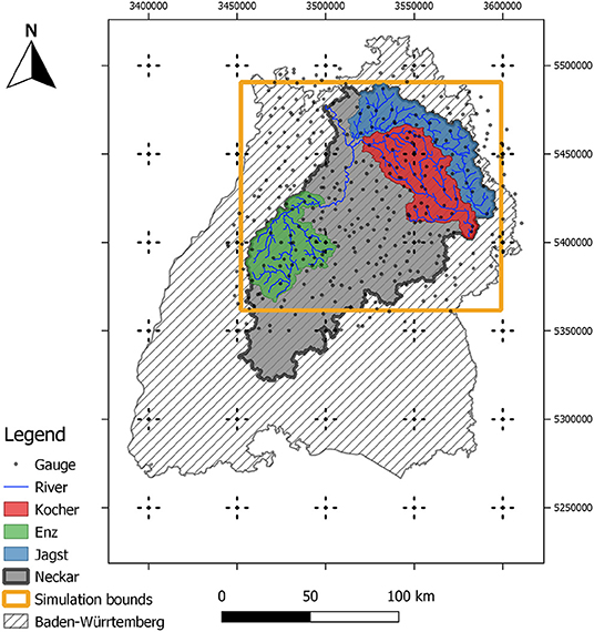
Figure 1. Study area showing the three considered sub-catchments of the Neckar river.

The total catchment area of the Neckar is about 14,000 km² while Enz, Jagst and Kocher have 1,655, 1,820, and 1,943 km², respectively. They are bounded by the Black Forest from the West and the Swabian Alps from the East. The mean annual interpolated precipitation for each is 928, 818, and 887 mm. Precipitation is relatively evenly distributed over the catchments. The mean areal interpolated temperatures are 11.7, 11.5, and 11.7 ^oC, respectively for the considered time period of 1991–2015 (9,131 days). Their elevations lie between 205–992, 155–731, and 159–745 meters above the mean sea level, respectively. The Jagst and the Kocher have elongated catchment forms, thus likely to have different precipitation variability than the roundish catchment like the Enz.

3.2. Data

Observed weather data time series were downloaded from the Deutscher Wetter Dienst's (DWD, German Weather Service) open access portal (DWD, 2019). The considered variables were precipitation and temperature (daily minimum, maximum, and average). Stations near but outside the rectangle covering all three catchments were considered. The number of available constraining precipitation observations varied between 120 and 230. Thus, the coverage with precipitation observations was extremely good, and there was little room for precipitation alterations between the stations. The potential evapotranspiration was computed using the Hargreaves-Samani equation (Hargreaves and Samani, 1982). The daily discharge time series was downloaded from the open access portal of the Landesanstalt für Umwelt Baden-Würrtemberg (LUBW, Environmental agency of the federal state of Baden-Würrtemberg) (LUBW, 2020).

3.3. Rainfall-Runoff Models

The total number of inversion time steps (number of days of the total selected events) considered was 1,386 (15%) out of the possible 9,131. The events were selected in a sequence such that making changes to the current time step would have negligible effects on the next considered one.

Two spatially distributed hydrological models with a grid resolution of 1 km were used: SHETRAN (physically-based) and HBV (conceptual). The input data was also at a 1 km spatial resolution with a 1 day temporal resolution.

3.3.1. SHETRAN

SHETRAN is a freely-available distributed catchment hydrological modeling software based on the Système Hydrologique Européen (SHE) principles, which simulates surface and subsurface flows and their interactions on a 3D spatial grid (Ewen et al., 2000). It includes components for vegetation interception and transpiration, overland flow, variably saturated subsurface flow and channel-aquifer interactions. Solutions to the governing, physics-based, partial differential equations of mass and momentum are solved on a three-dimensional grid using finite-difference equations (https://research.ncl.ac.uk/shetran/). The model parameters were not calibrated with a classical optimization procedure. Instead, available data such as the digital elevation model, soil and land use maps were used to estimate the model parameters (Birkinshaw et al., 2010; Lewis et al., 2018). These were modified within the plausible range of uncertainty to produce reasonable water balances.

3.3.2. HBV

The HBV (Bergström, 1992) model is a conceptual model developed by the Swidish Meteorological and Hydrological Institute (SMHI) (Bergström and Forsman, 1973). It is widely used for hydrological simulations and is well known for its easy handle and light burden calibration. The model version used here is the modified version by IWS, University of Stuttgart. It was calibrated using the gridded precipitation, temperature, and potential evapotranspiration interpolated using Ordinary Kriging (Wackernagel, 2004) for the considered time period. It was set in a distributed manner such that all the cells had the same model parameters, but the input data for each of them were different. In the end, the runoff from each cell was summed up and scaled appropriately to produce a simulated discharge time series. The Differential-Evolution (Storn and Price, 1997) optimization scheme was used to find the optimum model parameters using the Nash-Sutcliffe efficiency (Nash and Sutcliffe, 1970) as the objective function.

4. Results

4.1. Single Catchment Inversion Results

Rectangular precipitation fields covering all three catchments of the size of 147 km × 130 km were used for the inversion. Precipitation amounts for a regular 1 km × 1 km grid were identified. Precipitation stations in the field and outside near the boundary were taken as conditioning points. This means that at the observation locations, the precipitation amounts of the fields were identical to the observed ones.

The methodology to find precipitation fields was first applied for each catchment separately. This is referred to as individual inversions in the rest of the text. Simulations with 10 different sets of random fields were performed. As the computation time of the SHETRAN model is non-trivial (about 1 h per run) only 10 to 50 full iterations were carried out. The model performance improved quickly after a few iterations, and the improvement slowed down gradually with the increase of the number of iterations. Using both the models, Figure 2 shows the values of the objective function as a function of the number of iterations for the simulations done for Kocher and Figure 3 for the Enz. It is apparent that the sum of squared-differences decreases to about half of that obtained using interpolated precipitation.

FIGURE 2

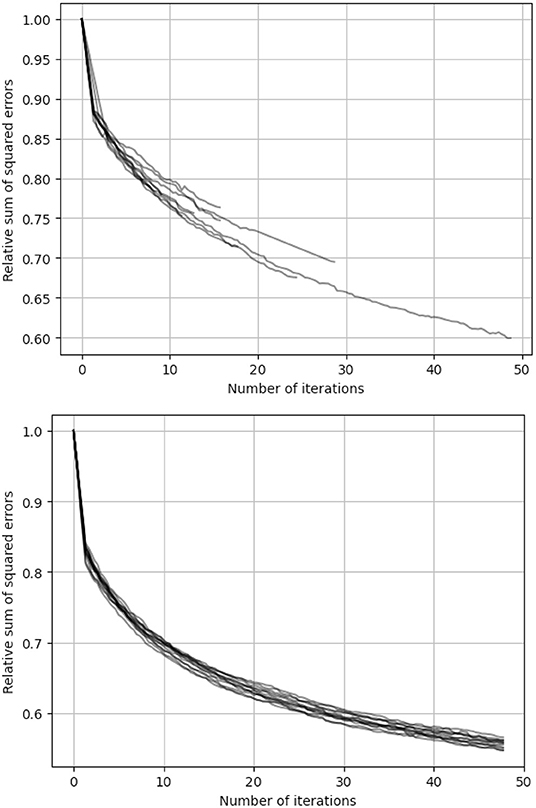
Figure 2. Relative sum of squared errors for the Kocher catchment as a function of the iterations completed for the 10 optimizations using SHETRAN (Top) and HBV (bottom). At iteration 0 the error corresponding to the interpolated precipitation is 1.0.

FIGURE 3

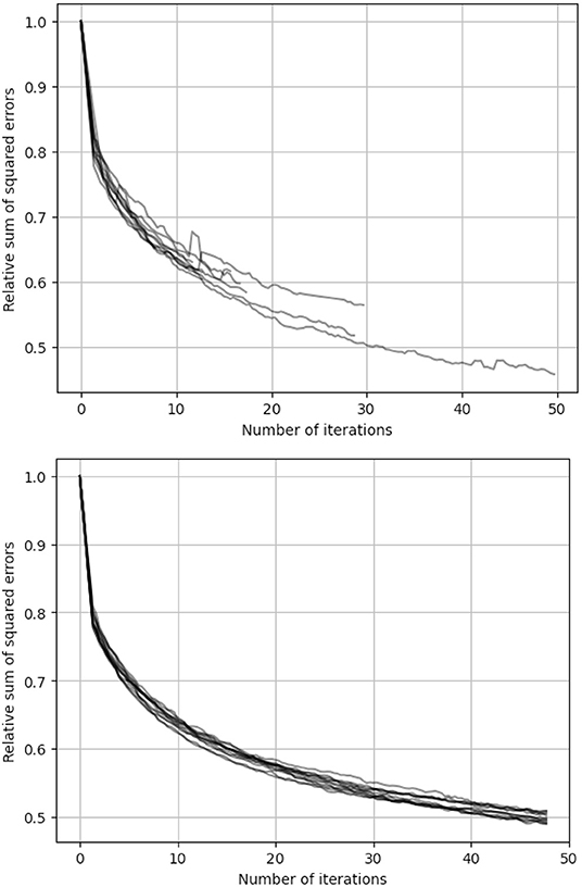
Figure 3. Sum of squared errors for the Enz catchment as a function of the iterations completed for the 10 optimizations using SHETRAN (top) and HBV (bottom). At iteration 0 the error corresponding to the interpolated precipitation is 1.0.

Tables 1, 2 show the Nash-Sutcliffe values and the sum of squared-differences for the interpolated and for the inverted precipitation obtained applying the final precipitation fields obtained by the algorithm using SHETRAN and HBV. Again, it can be seen that the inversion improves the model significantly. The mean squared error decreased by 40–50%. More iterations could further decrease the error. However, there is a danger of over-fitting (over-inverting) the precipitation fields. In order to test the robustness of the inversion, the inverted precipitation series of fields were applied to the other two catchments. Tables 3, 4 show the results for the final iterations. All values are slightly better than the ones obtained using interpolation. This means that adjusting precipitation for one catchment is not at the expense of another catchment. In fact, for the two close catchments Kocher and Jagst, the inversion of the precipitation for one catchment led to a significant improvement for the other. For Enz, the effect is much smaller, which is due to its distance to the other two catchments. Improvements are similar for both hydrological models.

TABLE 1

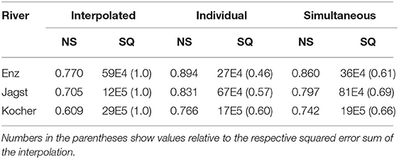
Table 1. Best model performance using interpolated, individually and simultaneously inverted precipitation with SHETRAN.

TABLE 2

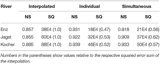
Table 2. Best model performance using interpolated, individually and simultaneously inverted precipitation with HBV.

TABLE 3

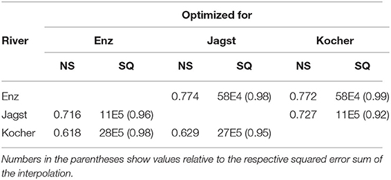
Table 3. Final model performance using precipitation inverted for a different catchment with SHETRAN.

TABLE 4

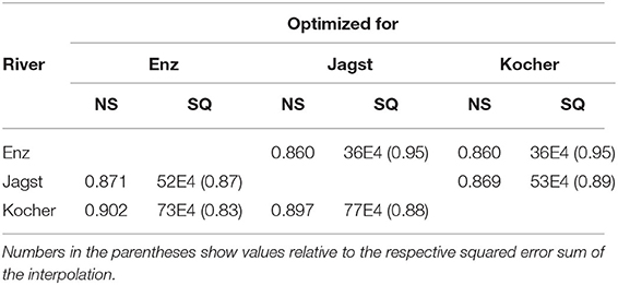
Table 4. Final model performance using precipitation inverted for a different catchment with HBV.

Looking at individual flood events, for some events, the improvement of simulation is very large. Figure 4 shows the hydrographs for an event obtained using interpolated vs. inverted precipitation. One can see that the severe underestimation of the hydrograph can be well explained by precipitation error. Figures 5–8 show the corresponding precipitation fields. Note that all fields are similar to the interpolated field, which is due to the dense precipitation measurement network. The number of stations used as constraints varied between 120 and 230. Even this high density of stations leaves room for variations. The details in between the stations are responsible for a large portion of the difference of the simulated discharge compared to the interpolation based discharge estimates. In some cases, only partial improvement could be achieved. Figure 9 shows an example of a flood event where the first peak could not be improved, while plausible precipitation fields were found for the second one. The corresponding fields are shown in Figures 10, 11. They show high similarity due to the large number of constraining observations, but the variability between the observations could explain the underestimation obtained when using interpolated precipitation. These results suggest that small differences in the precipitation fields may explain a large portion of the output uncertainty of the hydrological models.

FIGURE 4

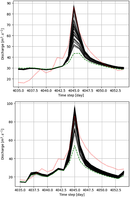
Figure 4. Discharge of Enz observed (dotted line) simulated using interpolated precipitation (dashed line) and simulated using individual model inversions (solid lines). Top, SHETRAN; bottom, HBV.

FIGURE 5

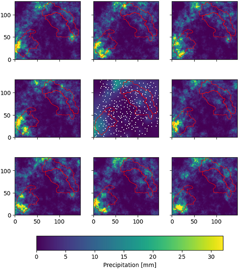
Figure 5. Eight inverted precipitation realizations for the Enz discharge for day 4,043 (January 27, 2002) and the interpolated precipitation in the middle using SHETRAN. The white squares in the middle figure represent the observation locations.

FIGURE 6

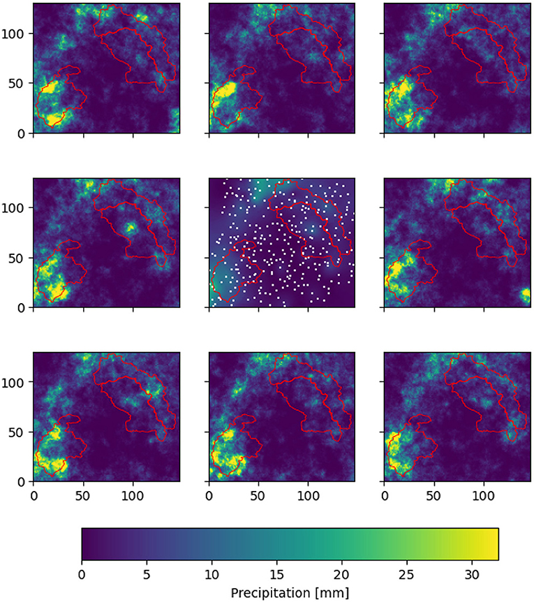
Figure 6. Eight inverted precipitation realizations for the Enz discharge for day 4,043 (January 27, 2002) and the interpolated precipitation in the middle using HBV. The white squares in the middle figure represent the observation locations.

FIGURE 7

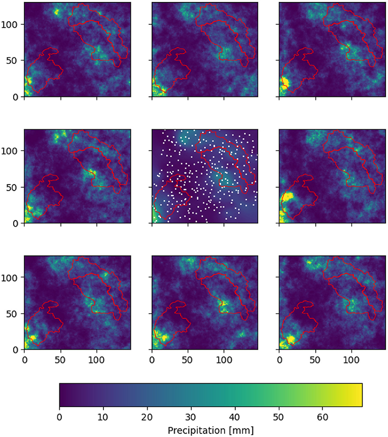
Figure 7. Eight inverted precipitation realizations for the Enz discharge for day 4,044 and the interpolated precipitation in the middle using SHETRAN. The white squares in the middle figure represent the observation locations.

FIGURE 8

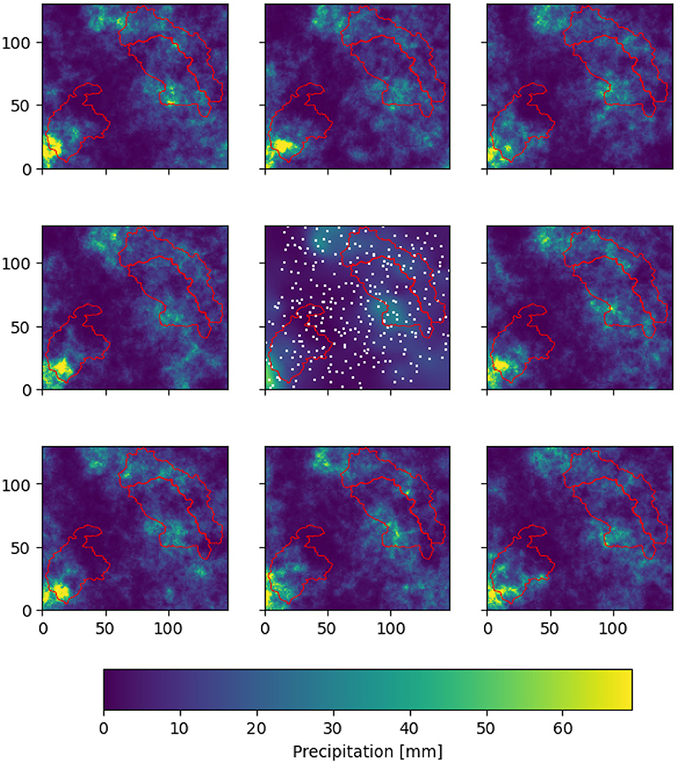
Figure 8. Eight inverted precipitation realizations for the Enz discharge for day 4,044 and the interpolated precipitation in the middle using HBV. The white squares in the middle figure represent the observation locations.

FIGURE 9

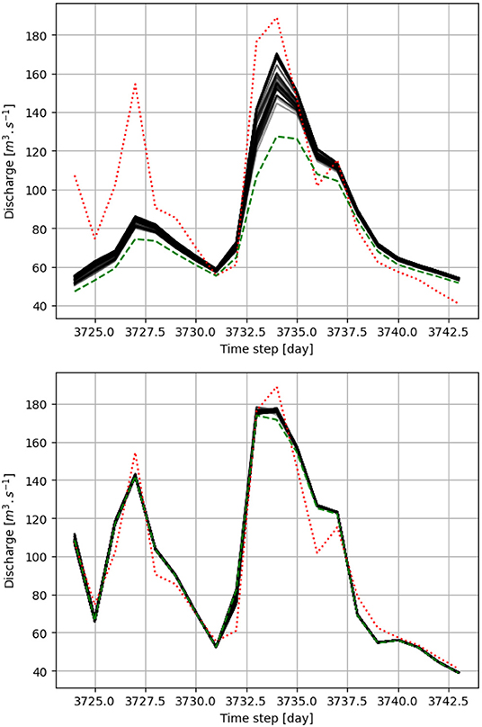
Figure 9. Discharge of Kocher observed (dotted line) simulated using interpolated precipitation (dashed line) and simulated using individual model inversions (solid lines). Top, SHETRAN; bottom, HBV.

FIGURE 10

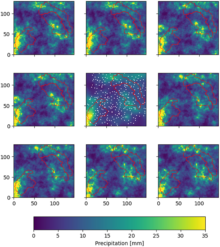
Figure 10. Eight inverted precipitation realizations for the Kocher discharge for day 3,733 (March 20, 2001) and the interpolated precipitation in the middle using SHETRAN. The white squares in the middle figure represent the observation locations.

FIGURE 11

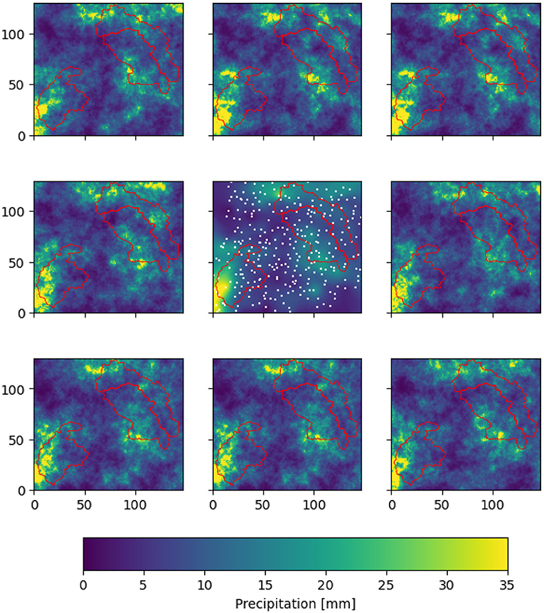
Figure 11. Eight inverted precipitation realizations for the Kocher discharge for day 3,733 (March 20, 2001) and the interpolated precipitation in the middle using HBV.

The reasons for little or no improvement for some events can vary. One of the plausible reasons is that even the relatively dense observation network may miss the heavy precipitation intensities, and the values measured at the stations may not be representative of the real precipitation. This kind of effect is not considered in the present methodology, where the distribution of the precipitation measured at the stations is taken as the distribution of precipitation over the whole field for each day.

In most (about 80%) of the cases, improvements were achieved when discharge was underestimated by the interpolation-based field. However, in about 20% of the cases, an overestimation was corrected. We suggest this is because observation networks are more likely to miss the maxima which occurred, than to capture them.

4.2. Results of the Simultaneous Inversion for the Three Catchments

In order to see to what extent the consideration of the discharge of several catchments constrains the adjustments of the precipitation fields, a joint inversion was carried out. Table 1 shows the performance of the model for the three catchments obtained by simultaneous inversion. The improvement is less than that with the same number of iterations for the individual catchments, but one can find precipitation fields which fulfill the conditions (observed values and spatial variability) that lead to a significant improvement for all catchments. These are referred to as simultaneous inversions in the rest of the paper.

Figures 12, 13 show an example of discharge using simultaneous inversion for the same event shown in Figure 9 using individual inversion. The model performances are similar, but the precipitation fields in Figures 12, 13 are different. The precipitation fields corresponding to the simultaneous inversion are more similar to each other due to the stronger constraints imposed by the discharge of the three catchments. Figure 14 shows the corresponding event hydrographs.

FIGURE 12

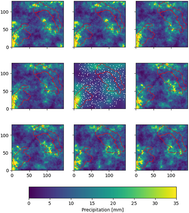
Figure 12. Eight inverted precipitation realizations for the simultaneous discharge for day 3,733 (March 20, 2001) and the interpolated precipitation in the middle using SHETRAN. The white squares in the middle figure represent the observation locations.

FIGURE 13

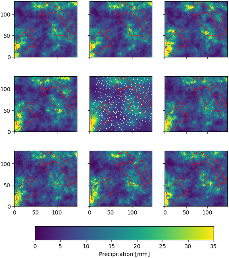
Figure 13. Eight inverted precipitation realizations for the simultaneous discharge for day 3,733 (March 20, 2001) and the interpolated precipitation in the middle using HBV. The white squares in the middle figure represent the observation locations.

FIGURE 14

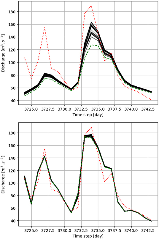
Figure 14. Discharge of Kocher observed (dotted line) simulated using interpolated precipitation (dashed line) and simulated using simultaneous model inversions (solid lines). Top, SHETRAN; bottom, HBV.

4.3. Results for Switched Inversion Precipitation

The results for the cases in which inverted precipitation obtained using one model was used as input for another model were also compared. Table 5 shows the change in model performances when the same catchment precipitation inverted using SHETRAN was used as an input for HBV. The results show slight improvements, showing that the models may have common problems with falsely estimated precipitation. Calibration of the HBV model leads to a partial error compensation, which can only be improved in some clear cases of for days with under or overestimation of precipitation. Table 6 shows the results for the case when other than the considered catchments were used for inversion. In this case, there is no improvement visible, which may be caused by the error compensation of the HBV model. We assume that if the HBV would be recalibrated for this realization of precipitation, the performance would also increase.

TABLE 5

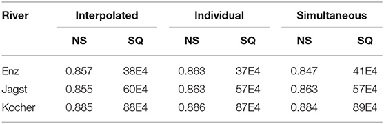
Table 5. Model performance comparison when using inverted precipitation from SHETRAN as an input for the HBV for the same catchment.

TABLE 6

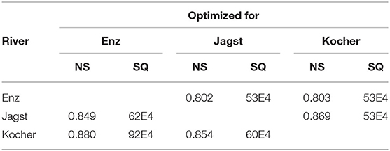
Table 6. Model performance comparison when using inverted precipitation from SHETRAN as an input for the HBV for the other catchments.

4.4. Comparison of Simulated Fields

Standard deviations for each time step using all simulated precipitation fields were computed to show the variability of the fields. Figures 15, 16 show standard deviation fields for the day 3,733 (March 20, 2001) using the simultaneous inversion for the three catchments for SHETRAN and HBV, respectively. According to the methodology, the standard deviations are zero at the observation locations as the fields were conditioned at those points. Both figures show that the uncertainty increased as the distance of unconditioned points increased from the conditioning ones. Interestingly, we saw no other pattern (preferential paths or otherwise) neither in SHETRAN nor in HBV. The standard deviations were higher near the boundaries and at locations with low observation density.

FIGURE 15

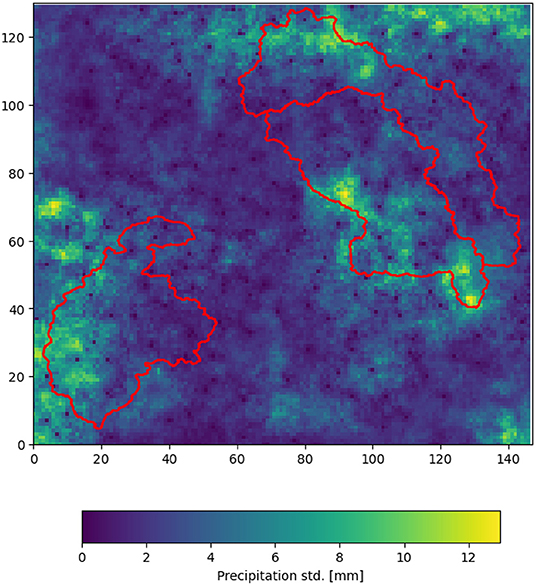
Figure 15. Standard deviation field of all realizations obtained using simultaneous inversion with SHETRAN for day 3,733 (March 20, 2001).

FIGURE 16

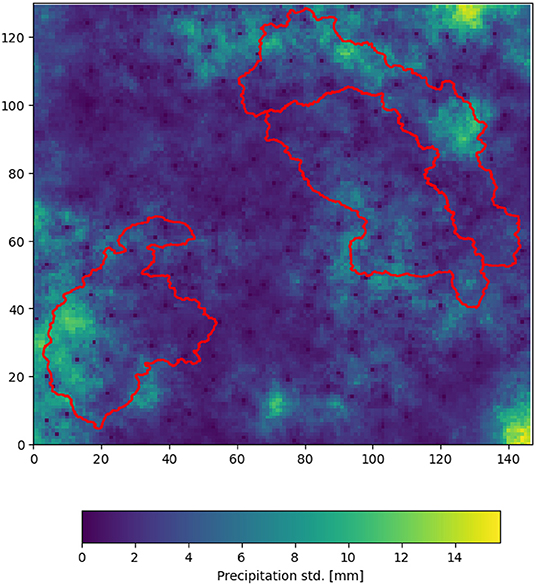
Figure 16. Standard deviation field of all realizations obtained using simultaneous inversion with HBV for day 3,733 (March 20, 2001).

Furthermore, the Root-mean-squared-error (RMSE) of all simulations at each pixel with respect to the interpolated field was also calculated. Figures 17, 18 show these fields for the same settings as that of the standard deviations.

FIGURE 17

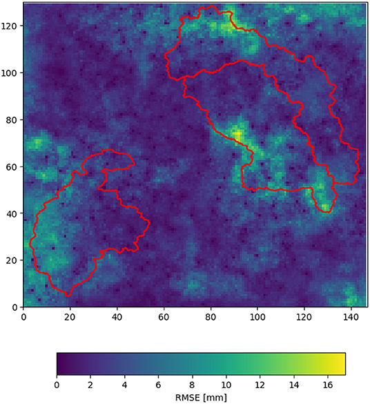
Figure 17. Root-mean-squared-error (RMSE) field of all realizations obtained using simultaneous inversion with SHETRAN for day 3,733 (March 20, 2001) with respect to the interpolated field.

FIGURE 18

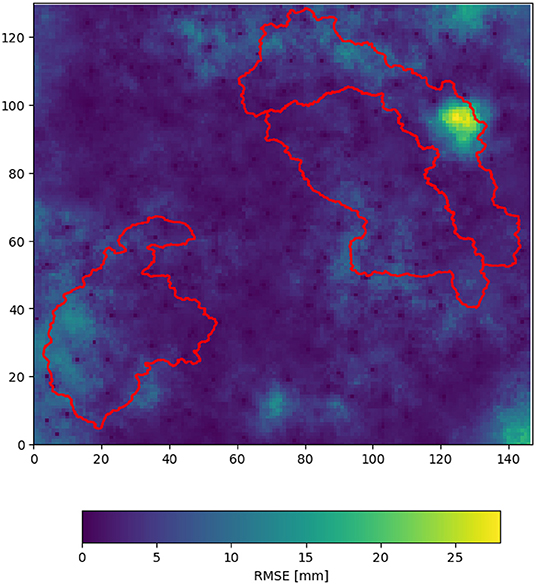
Figure 18. Root-mean-squared-error (RMSE) field of all realizations obtained using simultaneous inversion with HBV for day 3,733 (March 20, 2001) with respect to the interpolated field.

In order to quantify the similarity of the patterns for each simulated day, the Pearson correlations between all possible pairs of realizations were calculated. The mean correlation between the simulated precipitation fields corresponding to the same day is 0.68. This is mainly due to the conditioning by the observations and the assumption of spatial continuity reflected by the prescribed variogram. The different forms and sizes of the catchments expressed by the variance correction factor (f_t) (Isaaks and Srivastava, 1989) for catchment G is:

$\begin{array}{ll}{f}_t=1-\frac{\overline{{\gamma }_t(G,G)}}{{\sigma }_t^2}=1-\frac{{\displaystyle {\int }_G}{\displaystyle {\int }_G}{\gamma }_t(x-y)dxdy}{{\sigma }_t^2}& (5)\end{array}$

which expresses the variance of the areal mean precipitation compared to the variance of the point precipitation ${\sigma }_t^2$ for a given day t. Here, γ_t(h) is the variogram of precipitation on day t. For a typical variogram the values of the variance correction factor are 0.2858 for the Enz, 0.2053 for the Jagst and 0.2513 for the Kocher. The reduction of the mean squared error is related to this factor–the highest reduction of the model error is achieved for the Enz catchment, which has the highest reduction factor.

5. Discussion and Conclusions

In this contribution, the role of precipitation uncertainty and error on the discharge obtained using two hydrological models was investigated. Instead of simple sensitivity studies, it was intended to find out whether one can find time series of precipitation fields with high spatial resolution such that they reflect both the observed values and their spatial variability and also produce calculated discharges that are similar to the observed. Observed data from spatially dense networks (120 to 230 gauges) were used for constraining the precipitation fields. The results show that the overall squared-differences sum decreased by 40–50% while peak errors decreased by up to 70–90%. The inverted precipitation fields are very similar overall to the eye, but small differences had a major impact on discharge peaks. The inverted fields are non-unique, and a large number of different fields are found which can improve model performance. It was also shown that precipitation fields optimized using one model improved the results of the other to some extent, but they never became worse, compared with using the interpolated precipitation. Optimizing precipitation for a target catchment improved the results for the neighbor as well, but not for a more distant one. As the results for both models were improved significantly, it shows that the method has generality across conceptual and physically-based model types with different process representations.

Furthermore, the same methodology could be applied to find precipitation fields in higher (e.g., 1 h) temporal resolutions. For such a case, a space-time simulation has to be performed and advection (which is visible only in higher resolution fields such as those obtained using Radar) of the fields has to be incorporated as an additional constraint in the simulation methodology. We assume that much better modeling performance can be achieved using the appropriate temporal scales responsible for runoff formation. For mesoscale catchments, a temporal resolution of 1 h is much better for the description of the real hydrological processes, but due to the high variability of precipitation, present observations cannot provide useful estimates in space and time.

From our results we draw the following conclusions:

• Rainfall-runoff models may be better performing than we think, as the uncertainty of the calculated discharge can be, to a large extent, caused by inaccurate precipitation estimation.

• Assigning all uncertainty to the model parameters neglects this important part of the uncertainty.

• Discharge measurements can be used to improve precipitation estimation indirectly.

The methodology of this paper could also be used on other spatial and temporal scales, for example for global hydrological data assessment so that precipitation and discharge estimates are not independently assessed but harmonized with the help of water balance modeling.

We conclude that the uncertainty of model parameters and input uncertainty should both be considered. Precipitation uncertainty can be responsible for output uncertainty of up to 50% even in densely monitored catchments.

While the methodology can generate plausible precipitation fields which improve overall model performance, we have so far not established if these “better” fields have any characteristics which are physically meaningful, and related to correcting systematic errors in observation or interpolation, e.g., elevation dependence or wind-driven undercatch of gauges, rather than purely random errors due to under-sampling of the true field. A larger and more diverse range of catchments and topography is needed to investigate this aspect, which may then potentially lead to a practical outcome of guided improvement of precipitation fields and model performance in an operational predictive setting, rather than just establishing the potential for improvement.

Data Availability Statement

Publicly available datasets were analyzed in this study. This data can be found here: https://opendata.dwd.de/climate_environment/CDC/observations_germany/climate/daily/.

Author Contributions

AB and CK: conceptualization. AB, NW, and FA: data preparation. AB, SB, and NW: SHETRAN modeling. FA: HBV modeling. AB and FA: inverse modeling methodology. AB, CK, SB, NW, and FA: final manuscript preparation. All authors contributed to the article and approved the submitted version.

Funding

The authors acknowledge the financial support of the research group FOR 2416 Space-Time Dynamics of Extreme Floods (SPATE) by the German Research Foundation (DFG).

Conflict of Interest

The authors declare that the research was conducted in the absence of any commercial or financial relationships that could be construed as a potential conflict of interest.

Publisher's Note

All claims expressed in this article are solely those of the authors and do not necessarily represent those of their affiliated organizations, or those of the publisher, the editors and the reviewers. Any product that may be evaluated in this article, or claim that may be made by its manufacturer, is not guaranteed or endorsed by the publisher.

Acknowledgments

Python (van Rossum, 1995), Numpy (Harris et al., 2020), Scipy (Virtanen et al., 2020), Matplotlib (Hunter, 2007), Pandas (Wes McKinney, 2010; The Pandas Development Team, 2020), Pathos (McKerns et al., 2012), PyCharm IDE, Eclipse IDE and PyDev. We are very thankful to Dr. Shervan Gharari and the two reviewers. Their comments helped us improve the overall text, add important references that we did not know about, and add more informative figures.

References

Bárdossy, A., Anwar, F., and Seidel, J. (2020). Hydrological modelling in data sparse environment: inverse modelling of a historical flood event. Water 12, 3242. doi: 10.3390/w12113242

CrossRef Full Text | Google Scholar

Bergström, S. (1992). The HBV model: its structure and applications. SMHI Reports Hydrology. SMHI.

Google Scholar

Bergström, S., and Forsman, A. (1973). Development of a conceptual deterministic rainfall-runoff mode. Nord. Hydrol 4, 240–253. doi: 10.2166/nh.1973.0012

CrossRef Full Text | Google Scholar

Beven, K., and Binley, A. (2014). Glue: 20 years on. Hydrol Process. 28, 5897–5918. doi: 10.1002/hyp.10082

CrossRef Full Text | Google Scholar

Birkinshaw, S. J., James, P., and Ewen, J. (2010). Graphical user interface for rapid set-up of shetran physically-based river catchment model. Environ. Model. Softw. 25, 609–610. doi: 10.1016/j.envsoft.2009.11.011

CrossRef Full Text | Google Scholar

DWD (2019). Available online : https://opendata.dwd.de/climate_environment/CDC/observations_germany/climate/daily/.

Ewen, J., Parkin, G., and O'Connell, P. E. (2000). Shetran: distributed river basin flow and transport modeling system. J. Hydrol. Eng. 5, 250–258. doi: 10.1061/(ASCE)1084-0699(2000)5:3(250)

CrossRef Full Text | Google Scholar

Gharari, S., Gupta, H. V., Clark, M. P., Hrachowitz, M., Fenicia, F., Matgen, P., et al. (2021). Understanding the information content in the hierarchy of model development decisions: learning from data. Water Resour. Res. 57, e2020WR027948. doi: 10.1029/2020WR027948

CrossRef Full Text | Google Scholar

Grundmann, J., Hörning, S., and Bárdossy, A. (2019). Stochastic reconstruction of spatio-temporal rainfall patterns by inverse hydrologic modelling. Hydrol. Earth Syst. Sci. 23, 225–237. doi: 10.5194/hess-23-225-2019

CrossRef Full Text | Google Scholar

Hargreaves, G., and Samani, Z. (1982). Estimating potential evapotranspiration. J. Irrigat. Drainage Division 108, 225–230. doi: 10.1061/JRCEA4.0001390

CrossRef Full Text | Google Scholar

Harris, C. R., Millman, K. J., van der Walt, S. J., Gommers, R., Virtanen, P., Cournapeau, D., et al. (2020). Array programming with NumPy. Nature 585, 357–362. doi: 10.1038/s41586-020-2649-2

PubMed Abstract | CrossRef Full Text | Google Scholar

Hörning, S., Sreekanth, J., and Bárdossy, A. (2019). Computational efficient inverse groundwater modeling using random mixing and whittaker–shannon interpolation. Adv. Water Resour. 123, 109–119. doi: 10.1016/j.advwatres.2018.11.012

CrossRef Full Text | Google Scholar

Hunter, J. D. (2007). Matplotlib: a 2d graphics environment. Comput. Sci. Eng. 9, 90–95. doi: 10.1109/MCSE.2007.55

CrossRef Full Text | Google Scholar

Isaaks, E., and Srivastava, R. (1989). An Introduction to Applied Geostatistics. Oxford University Press.

PubMed Abstract | Google Scholar

Kavetski, D., Kuczera, G., and Franks, S. (2006). Bayesian analysis of input uncertainty in hydrological modeling: 2. application. Water Resour. Res. 42, 4376. doi: 10.1029/2005WR004376

CrossRef Full Text | Google Scholar

Kirchner, J. (2009). Catchments as simple dynamical systems: catchment characterization, rainfall-runoff modeling, and doing hydrology backward. Water Resour. Res. 45, 6912. doi: 10.1029/2008WR006912

CrossRef Full Text | Google Scholar

Krier, R., Matgen, P., Goergen, K., Pfister, L., Hoffmann, L., Kirchner, J., et al. (2012). Inferring catchment precipitation by doing hydrology backward: a test in 24 small and mesoscale catchments in luxembourg. Water Resour. Res. 48, W10525. doi: 10.1029/2011WR010657

CrossRef Full Text | Google Scholar

Lewis, E., Birkinshaw, S., Kilsby, C., and Fowler, H. J. (2018). Development of a system for automated setup of a physically-based, spatially-distributed hydrological model for catchments in great britain. Environ. Model. Softw. 108, 102–110. doi: 10.1016/j.envsoft.2018.07.006

CrossRef Full Text | Google Scholar

LUBW (2020). Available online at: https://udo.lubw.baden-wuerttemberg.de/public/.

McKerns, M. M., Strand, L., Sullivan, T., Fang, A., and Aivazis, M. A. (2012). Building a framework for predictive science. arXiv preprint arXiv:1202.1056. doi: 10.25080/Majora-ebaa42b7-00d

CrossRef Full Text | Google Scholar

Nash, J., and Sutcliffe, J. (1970). River flow forecasting through conceptual models. 1. a discussion of principles. J. Hydrol. 10, 282–290. doi: 10.1016/0022-1694(70)90255-6

CrossRef Full Text | Google Scholar

Pianosi, F., and Wagener, T. (2016). Understanding the time-varying importance of different uncertainty sources in hydrological modelling using global sensitivity analysis. Hydrol. Process. 30, 3991–4003. doi: 10.1002/hyp.10968

CrossRef Full Text | Google Scholar

Schoups, G., and Vrugt, J. A. (2010). A formal likelihood function for parameter and predictive inference of hydrologic models with correlated, heteroscedastic, and non-gaussian errors. Water Resour Res. 46, W008933. doi: 10.1029/2009WR008933

CrossRef Full Text | Google Scholar

Stedinger, J. R., Vogel, R. M., Lee, S. U., and Batchelder, R. (2008). Appraisal of the generalized likelihood uncertainty estimation (glue) method. Water Resour Res. 44, W00B06. doi: 10.1029/2008WR006822

CrossRef Full Text | Google Scholar

Storn, R., and Price, K. (1997). Differential evolution – a simple and efficient heuristic for global optimization over continuous spaces. J. Glob. Optimizat. 11, 341–359. doi: 10.1023/A:1008202821328

CrossRef Full Text | Google Scholar

The Pandas Development Team (2020). pandas-dev/pandas: Pandas.

van Rossum, G. (1995). Python tutorial. Technical Report CS-R9526, Centrum voor Wiskunde en Informatica (CWI), Amsterdam.

Google Scholar

Virtanen, P., Gommers, R., Oliphant, T. E., Haberland, M., Reddy, T., Cournapeau, D., et al. (2020). SciPy 1.0: fundamental algorithms for scientific computing in python. Nat. Methods 17, 261–272. doi: 10.1038/s41592-020-0772-5

PubMed Abstract | CrossRef Full Text | Google Scholar

Wackernagel, H. (2004). “Ordinary kriging,” in Multivariate Geostatistics: An Introduction with Applications, Chapter 11 (Springer), 74–81.

Google Scholar

Wes McKinney (2010). “Data structures for statistical computing in python,” in Proceedings of the 9th Python in Science Conference, eds S. van der Walt and J. Millman, 56–61.

Google Scholar

Yatheendradas, S., Wagener, T., Gupta, H., Unkrich, C., Goodrich, D., Schaffner, M., et al. (2008). Understanding uncertainty in distributed flash flood forecasting for semiarid regions. Water Resour. Res. 44, W05S19. doi: 10.1029/2007WR005940

CrossRef Full Text | Google Scholar