 Swamini Khurana
 Falk Heße
 Anke Hildebrandt
 Martin Thullner
95% of researchers rate our articles as excellent or good
Learn more about the work of our research integrity team to safeguard the quality of each article we publish.
Find out more
ORIGINAL RESEARCH article
Front. Water , 24 March 2022
Sec. Water and Hydrocomplexity
Volume 4 - 2022 | https://doi.org/10.3389/frwa.2022.780297
This article is part of the Research Topic Uncertainty in Groundwater Modeling Across Scales View all 5 articles
The fluxes of water and solutes in the subsurface compartment of the Critical Zone are temporally dynamic and it is unclear how this impacts microbial mediated nutrient cycling in the spatially heterogeneous subsurface. To investigate this, we undertook numerical modeling, simulating the transport in a wide range of spatially heterogeneous domains, and the biogeochemical transformation of organic carbon and nitrogen compounds using a complex microbial community with four (4) distinct functional groups, in water saturated subsurface compartments. We performed a comprehensive uncertainty analysis accounting for varying residence times and spatial heterogeneity. While the aggregated removal of chemical species in the domains over the entire simulation period was approximately the same as that in steady state conditions, the sub-scale temporal variation of microbial biomass and chemical discharge from a domain depended strongly on the interplay of spatial heterogeneity and temporal dynamics of the forcing. We showed that the travel time and the Damköhler number (Da) can be used to predict the temporally varying chemical discharge from a spatially heterogeneous domain. In homogeneous domains, chemical discharge in temporally dynamic conditions could be double of that in the steady state conditions while microbial biomass varied up to 75% of that in steady state conditions. In heterogeneous domains, the interquartile range of uncertainty in chemical discharge in reaction dominated systems (log10Da > 0) was double of that in steady state conditions. However, high heterogeneous domains resulted in outliers where chemical discharge could be as high as 10–20 times of that in steady state conditions in high flow periods. And in transport dominated systems (log10Da < 0), the chemical discharge could be half of that in steady state conditions in unusually low flow conditions. In conclusion, ignoring spatio-temporal heterogeneities in a numerical modeling approach may exacerbate inaccurate estimation of nutrient export and microbial biomass. The results are relevant to long-term field monitoring studies, and for homogeneous soil column-scale experiments investigating the role of temporal dynamics on microbial redox dynamics.
Groundwater availability and quality are of great interest due its wide use as a source of irrigation and drinking water (World Water Assessment Programme, 2009; UNESCO and UN-Water, 2020). Groundwater quality (microbial community structure and physicochemical parameters) varies with time, environmental conditions, and a variety of forcing (Basu et al., 2010; Okkonen et al., 2010; Zhou et al., 2012; Rezanezhad et al., 2014; Yabusaki et al., 2017; Lohmann et al., 2020; Yan et al., 2021). Such forcing includes fluctuating groundwater head with time of the day, weather events, groundwater abstraction, or fluctuating leakage of carbon and terminal electron acceptors [such as dissolved oxygen (DO) and nitrate] with weather events or land use change (Khatri and Tyagi, 2015). It is beneficial to establish links between forcing and nutrient cycling in the groundwater, which may further assist in ensuring safe access to water resources.
Historical studies have established that temporal variations in nutrient cycling in subsurface systems are linked with diverse and dynamic bacterial communities, their variation being seasonal in nature with patterns recurring year on year, synchronously with environmental conditions and the forcing (Sinke et al., 1998; Kolehmainen et al., 2008; Moore-Kucera and Dick, 2008; Febria et al., 2010; Rezanezhad et al., 2014; Rudolf von Rohr et al., 2014; Vidal-Gavilan et al., 2014; Danczak et al., 2016; King et al., 2017; Zheng et al., 2019; Meng et al., 2021). For example, Pett-Ridge et al. (2013), Rezanezhad et al. (2014), Bhattacharyya et al. (2018) and Lohmann et al. (2020) displayed that microbial communities present in the periodically fluctuating redox zone are stable and switch between aerobic and anaerobic respiration according to fluctuating oxic-anoxic conditions, whereby saturated anoxic conditions induced anaerobic respiration and oxic unsaturated conditions induced aerobic respiration. This adaptation of microbial communities to metabolize varying nutrient inputs by harnessing varying energy gradients is based on the habitat and external forcing such as climate or precipitation pattern (Pett-Ridge et al., 2013). However, with higher uncertainty expected in these forcing in a changing climate (Easterling et al., 2000; Lambin et al., 2003; Trenberth et al., 2003, 2014; Cai et al., 2014; Cohen et al., 2014), any prediction of the response of subsurface microbial communities to temporally varying forcing based on aforementioned studies in hitherto unforeseen scenarios is associated with large uncertainty, resulting in limited capacity to assess mitigation strategies.
Prediction of spatio-temporally varying groundwater quality is further complicated by lack of high-resolution field data, that causes uncertainty in the parametrization of the reaction network and the flow regime. Furthermore, assumption of homogeneous and uniform conditions results in uncertainty in reactive transport modeling outcomes or predictions (Köhne et al., 2009; Sassen et al., 2012). For example, Berkowitz (2002) discusses in detail how inadequate field measurements result in uncertainty in parametrizing the fractured rock domain, further expanding on the inadequacy of simplified 1D or 2D models for accurate predictions. In reactive transport modeling, Shi et al. (2014) observed deviation as large as 40% of average simulation results and Nitzsche et al. (2000) observed an uncertainty band equivalent to median concentrations (of the chemical of concern) in drinking water, the variation resulting from uncertainty in the parametrization of their respective models. Recently, Ritschel and Totsche (2016) displayed that using closed flow columns experiments to derive reaction parameters (degradation) and flow parameters (dispersion) reduced the associated uncertainty by an order of magnitude. Evidently, use of low resolution field scale data and simplified, homogeneous steady state laboratory scale data to parametrize models results in high uncertainty in model predictions (Berkowitz et al., 2016), especially when upscaling the models to larger scales (Zhang et al., 2021).
With both temporal variations in forcing and characterization of field scale processes being subject to substantial uncertainty, we recognize the need to investigate how the temporal variation in nutrient cycling depends on either variation in forcing such as weather events, seasonal cycles, average flow rate or domain characteristics such as variation in the conductivity field or porosity. Leavitt et al. (2011), focusing on speciation of U(VI), already established that spatial uncertainty is a substantial contributor to model prediction errors. Chakrawal et al. (2020) further derived that predicted non-linear microbial respiration rate in heterogeneous domains is less than that in homogeneous domains. Neglecting spatial heterogeneity in conductivity of the subsurface matrix alone can result in prediction errors associated with removal of chemical species (dissolved organic carbon (DOC), dissolved oxygen (DO), nitrate, ammonium) between 60% and 500 times of that in homogeneous domains (Khurana et al., 2022). This uncertainty may be further exacerbated by neglecting temporal dynamics (Leavitt et al., 2011). Given the complex nature of natural systems with numerous confounding factors, we aim to disentangle the influence of temporal dynamics in groundwater head, and uncertainty thereof, on the ability of a diverse geomicrobial community to transform organic carbon (DOC) and nitrogen (nitrate and ammonium) compounds.
The aim of this study is to quantitatively assess the response of the dynamics of microbially mediated organic carbon and nitrogen turnover in the subsurface to temporal variations of the hydrological forcing (controlling the advective-dispersive transport of mobile species), and to determine the uncertainty resulting from neglecting such variations in model-based predictions of nutrient cycling. To investigate these questions, we use a reactive transport modeling approach allowing to impose defined conditions and their temporal and spatial variability. This allows to disentangle the interplay between the dynamics of key biogeochemical processes involved in the cycling of carbon and nitrogen and the dynamics of the hydrological forcing. For this purpose, we performed a series of reactive transport modeling experiments representing pristine, oligotrophic conditions in the groundwater considering its wide use as a source for irrigation and for drinking water (World Water Assessment Programme, 2009; Siebert et al., 2010). We used the novel and comprehensive reaction network developed by Khurana et al. (2022) to simulate scenarios that combined different levels of temporal fluctuations of the forcing, groundwater head in our study, with those of subsurface heterogeneities (Khurana et al., 2022) to determine the variability in the export of carbon and nitrogen from subsurface systems. We assumed that the groundwater head fluctuates in response to diurnal, seasonal and inter-annual cycles in atmospheric conditions. Deep percolation from surface into the deeper subsurface depends furthermore on dry and wet seasons, affecting groundwater heads. The transformation of carbon and nitrogen compounds in our in-silico system is mediated by aerobic autotrophs and heterotrophs, as well as anaerobic heterotrophs. Since we use a complex microbial community comprising species using multiple respiration strategies and study its response to temporal fluctuations at several scales (diurnal to seasonal) in a variety of flow regimes, the results help estimate the uncertainty in nutrient discharge in a wide range of sub-surficial microbial reactive systems. We are thus able to identify subsurficial reactive systems where spatio-temporal heterogeneities contribute to large uncertainty in transient conditions at field scales and estimate this associated uncertainty. This, in turn, may contribute toward improved decision making with respect to the spatial resolution of model domain, and spatio-temporal resolution of field data collection, consequently improving the predictability of reactive transport models in transient conditions at field scales.
We used a numerical reactive transport modeling approach to investigate the impact of temporal variation in groundwater flow rates on nutrient cycling in the groundwater, with a focus on organic carbon and nitrogen. For this we considered diurnal fluctuations, seasonal, and inter-annual cycles in flow velocity in conjunction with varying spatial heterogeneity of the aquifer. We used conditions from our subject site (Küsel et al., 2016; Kohlhepp et al., 2017) in Hainich National Park, located in the Nägelstedt catchment in central Germany [a Critical Zone Exploratory of the Collaborative Research Center (CRC) AquaDiva 1076] to inform the development and parametrization of the model so that both, the model and the investigated scenarios, are physically plausible. The subject site spans forest, grassland and agricultural areas, and is underlain by multiple stories of limestone aquifers. The groundwater monitoring wells tap the groundwater at varying depths. Thus, long term hydrobiogeochemical observations across the site below varying land-use types are available.
The model comprised a transport component and a reactive component representing microbial mass-transfer processes (called process network from hereon) in spatially heterogeneous and fully saturated domains (0.5 m × 0.3 m in size) subjected to temporal fluctuations in groundwater head at the inlet of the domain resulting in variation in groundwater velocities imposed in the domain. The size of the domain matched the scale of a typical groundwater monitoring well screen (meter to sub-meter scale). Unless specifically low-flow sampling techniques are used, spatial heterogeneity at the scale lower than the monitoring well screen is seldom resolved. Thus, we deemed this scale of the domain to be appropriate for our study.
Overall, we considered three different flow regimes. We imposed an average groundwater velocity of 3.8 10−4 m d−1, matching the average recharge associated with the subject site (Jing et al., 2018) in the domain, which was adopted as the slow flow regime here. The average groundwater velocity was increased by a factor of 10 in the medium flow regime and by a factor of 100 in the fast flow regime, to capture a wider variety of subsurface systems with different water flux rates [also used by Rein et al. (2009)]. This resulted in the residence time (synonymously used as breakthrough time) of a conservative tracer in steady state conditions in a homogeneous domain to be 230 days in the slow flow regime, 28 days in the medium flow regime and 3 days in the fast flow regime.
Since we aim to study the uncertainty induced due to unresolved spatio-temporal heterogeneities, we set up a wide range of physically plausible spatially heterogeneous domains (Section Spatially heterogeneous domains in Methods) and subjected all of these systems to temporal dynamics (Section Temporal dynamics: Simulated scenarios). We compared the variation in the response of these systems from that of homogeneous domains (details in Section Data analysis).
We used the same conceptual approach used in Khurana et al. (2022) to describe the reactive processes controlling the fate of organic carbon and nitrogen compounds in the domain. A detailed explanation of the complete process network is available in Khurana et al. (2022) and summarized here (Figure 1).
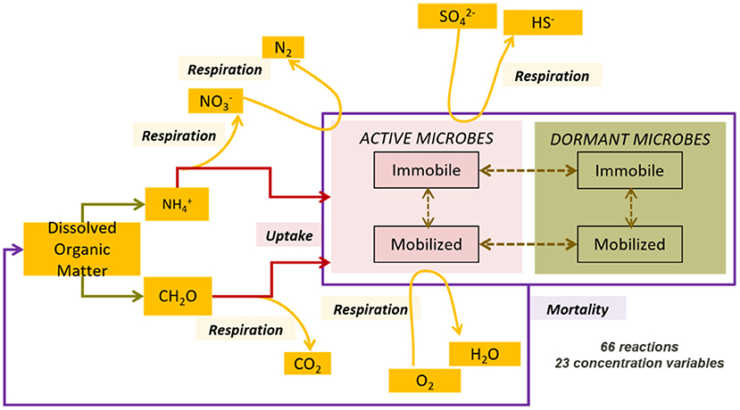
Figure 1. Complex process network comprising aerobic and anaerobic microbial species in both active and inactive states, both immobilized on the matrix and mobilized in the groundwater, reproduced from Khurana et al. (2022).
The process network captured a variety of microbial functional groups: aerobic dissolved organic carbon (DOC) degraders, nitrate reducing DOC degraders, sulfate reducing DOC degraders, and finally ammonia oxidizers. The process network, hence, accounted for both heterotrophy and autotrophy in the subsurface, in both aerobic and anaerobic conditions. These microbial groups mediate the transformation of DOC, DO, nitrate, ammonium, and sulfate in the subsurface. Thus, we were able to explore the removal of all of these chemical species in the model.
In addition to growth and respiration, we also included additional microbial life processes such as dormancy and reactivation, immobilization on the medium and mobilization into the groundwater, and mortality. These processes affected the access of microbial species to suitable carbon source and energy gradients. Additionally, capturing active and inactive biomass or mobile and immobilized biomass separately assisted in developing an understanding of the biogeochemical potential of subsurface systems, and their response to changing hydrological settings. We summarized the components and associated processes in the process network in Table 1.
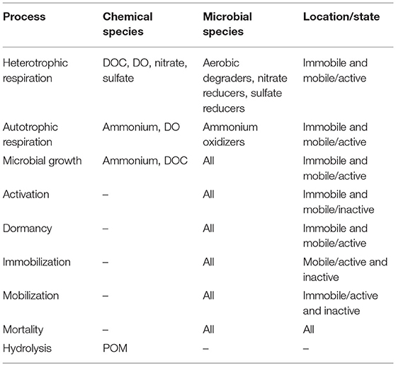
Table 1. Summary of process network: components, acting microbial species, and processes.
We generated spatially heterogeneous domains using a combination of variance (we used 0.1, 1, 5, and 10 as variance) and anisotropy (we used 2, 5, and 10 as anisotropy) in the log conductivity field to enforce spatially variable flow conditions. This approach is well-established to describe spatial heterogeneity in porous media (de Marsily et al., 2005). The combination of variance and anisotropy (in total yielding 12 scenarios) effectively captured a variety of heterogeneous domains. We generated four spatial random fields in each scenario, thus yielding 48 spatially heterogeneous domains and one homogeneous domain. Spatial heterogeneity resulted in a reduction of breakthrough time of a conservative tracer. The resulting breakthrough time was as low as 20% of the breakthrough time in the corresponding homogeneous domain, depending on the flow regime and intensity of spatial heterogeneity in the domain. A detailed explanation of the rationale and tools used to generate spatially heterogeneous fields, and effect of spatial heterogeneity on breakthrough time is available in Khurana et al. (2022).
We conceptualized three scenarios to enforce temporal dynamics in the forcing. Groundwater head (and consequently flow rate) was observed and recorded over a period of decades in the Nägelstedt catchment (the relevant catchment for the subject site). The time series analysis of the varying groundwater head data [presented by Jing et al. (2018)] revealed it to be a multi-variate Gaussian distribution with an exponential like covariance model. Hence, we generated three synthetic time series of groundwater head based on this. Herein, we used an exponential covariance model, varying the value of the variance (using 1,2, and 5 m2) and correlation time scale to incorporate annual [or seasonal with length scale as 365 days, referred to as g1(t)] and super-annual cycles [with length scale as 730 days, 2 years, referred to as g2(t)] in the groundwater head. We superimposed the time series g1(t) and g2(t) generated using the two length scales for the same variance and centered the mean of the distribution around 1 using Equation 1:
where, μ is the mean of the sum of g1(t) an g2(t). The product of this time series [f(t)] with the head at the inlet for each scenario was then applied at the inlet of the domain as the temporally varying forcing. Thus, the three imposed time series showed varying characteristics (Table 2). The covariance of the mean-adjusted time series varied between 0.15 and 0.27. For the first time series, the memory (the time lag when autocorrelation reduced to below 0.7, see section Cross-correlation, memory, and backward traceability) was 39 days, while for the third time series with the highest covariance, the memory was 166 days. See Supplementary Figure 1 for the autocorrelation function.
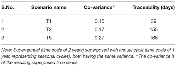
Table 2. Summary of temporally dynamic scenarios investigated.
We simulated a period of 15 years to evaluate the impact of temporal dynamics. The initial conditions for these simulations were steady state conditions induced in each domain as described in Khurana et al. (2022). Even though the water flux varied in time to simulate temporal dynamics; the time averaged water flux in each domain was constant for each flow regime (i.e., slow, medium, and fast flow regime) over the entire simulation period of 15 years for the purposes of keeping the results of the simulations comparable. All the domains were subjected to three different series of temporal variations in flow rate (Table 2). In total, we ran 441 simulations: three time series scenarios imposed on 48 spatially heterogeneous domains and one homogeneous domain in three different flow regimes.
We used OGS#BRNS (Aguilera et al., 2005; Centler et al., 2010; Kolditz et al., 2012) as the numerical modeling tool. This tool has been used successfully to simulate a complex reaction network combined with a variety of spatially heterogeneous geologic settings (Centler et al., 2013; Khurana et al., 2022). We further leveraged this tool in this study to include a variety of temporally dynamic conditions. Using a constant finite volume discretization of 0.01 m in both directions, we performed transient simulations for a period of 15 years.
We used the Python programming language (van Rossum and Drake, 2006), referred to as Python henceforth, for the entire workflow of the study. We set up the scenarios for running the simulations using OGS#BRNS using ogs5py package (Müller et al., 2021b). We used the GSTools package (Müller et al., 2021a) to generate the spatial random fields to represent heterogeneous domains in OGS#BRNS [also described in Khurana et al. (2022)] and also to generate the temporally changing groundwater head at the inlet of the domain. We processed and further analyzed simulation results using a workflow in Python as well. We used Python to generate all graphical outputs presented in this paper for ease of reproducibility.
We recorded observations at a time interval of 5 days in all scenarios. We extracted the following response variables from the simulation results:
1. Chemical/reactive species: Normalized flux averaged concentration of each chemical species leaving the domain (DOC, DO, nitrate, ammonium, total nitrogen, total organic carbon as mentioned in Table 1), and
2. Microbial biomass: Normalized total biomass of each microbial species in the domain.
We then explored the impact of temporal dynamics in changing groundwater head at the inlet boundary on these time series by characterizing the cross-correlation, backward traceability, and responsiveness as defined below. We compared these simulation results with base cases (detailed below) to evaluate the impact of spatio-temporal heterogeneity (base case being homogeneous domains in temporally dynamic conditions) and the impact of temporal dynamics (base case being spatially heterogeneous and homogeneous domains in steady state conditions). In this way, we were able to estimate the uncertainty induced by both spatial heterogeneity and temporal dynamics.
We used time lagged cross-correlation (Pearson), and particularly the peak value (referred to as R hereon), to investigate how strongly the response variables are linked with the temporal dynamics at the inlet boundary of the domain. We adapted classification of correlation into strong, moderate and weak types from Moore et al. (2013) and Lehmann et al. (2021). Weak correlation (−0.4 ≤ R ≤ 0.4) indicates that the value did not follow closely the head signal at the inlet. If the R > 0.7, then it is strongly correlated with the forcing, indicating that the response variable is changing according to the forcing.
Temporal variations in a time series signal are linearly traceable when the autocorrelation of the time series is strong even over a time lag. We termed the time point (in days) after which the lag autocorrelation falls below 0.7 as “memory” of the time series signal. We used memory to characterize the forcing.
A traceable linear relation also exists between the forcing and the response variables as long as the lag cross-correlation is strong even over a time lag. We termed the time point (in days) after which the lag cross-correlation falls below 0.7 as “backward traceability.” In other words, backward traceability indicated the duration of the impact of the forcing on response variables of a system.
We consider the response of the system to temporal dynamics to be less uncertain, given a high correlation and short backward traceability. Alternatively, a lack of correlation between the response of the system and hydrological settings indicates the relative stability of the system and its inertia to external disturbances, rendering the system behavior to be more certain.
We referred to the root mean squared amplitude of the response variables' time series signals resulting from temporally dynamic forcing as responsiveness for brevity. Responsiveness was calculated using Scipy package (Virtanen et al., 2020) as explained in Equation (2):
where the power spectral density is related with the autocovariance of the time series Cnorm(t), as introduced by Duffy and Gelhar (1985) and Cnorm is defined using Equation (3):
where Cout(t) is the time series signal of the response variables at the outlet and Cout,base is the concentration of the same chemical species at the outlet in steady state conditions. To assess the responsiveness of spatially heterogeneous domains specifically, we normalized it by the responsiveness of corresponding base case (homogeneous domains in temporally dynamic conditions) using Equation 4:
where, a normalized amplitude of 100% indicates that the spatially heterogeneous domain has the same amplitude as the homogeneous domain, given the same temporal dynamics in the forcing, rendering the system behavior to be less uncertain with respect to spatial heterogeneity. In contrast, the response of the system is uncertain if the responsiveness is high, and cannot be substituted by a similar homogeneous domain, rendering the system behavior to be more uncertain.
We used the Damköhler number to characterize reaction regimes (Pittroff et al., 2017; Khurana et al., 2022) in steady state conditions to generalize results and to move away from domain specific, flow regime specific, chemical, or microbial biomass specific discussions. To estimate Da, we assigned the characteristic transport time scale as the breakthrough time, assigned the characteristic reaction time scale as the time taken for 63% loss in chemical species concentration and took their ratio. If the chemical species concentration at the outlet is higher than 5% of the inlet concentration, the estimation of Da reduced to Equation (5) using the above definitions (Khurana et al., 2022).
with Cin [L−3 N] as flux averaged concentration of a chemical species entering the domain, and Cout [L−3 N] as flux averaged concentration of the chemical species leaving the domain in steady state conditions (that is the initial conditions in the simulation). If the chemical species concentration at the outlet is <5% of the inlet concentration, we derived the characteristic reaction time scale by identifying the cross-section where 95% loss of chemical species occurs, deriving the tracer breakthrough time at this cross-section and using 63% loss in chemical species to calculate the characteristic reaction time scale (Khurana et al., 2022):
where, Cy5 is the concentration of the chemical species at the point where (y = y5) 95% loss in chemical species occurs, τy5 is the breakthrough time for a conservative tracer at this point. Using the breakthrough time of the tracer at the outlet of the domain, we then estimated the Da in systems where the chemical species were fully (>95% loss) consumed at the outlet of the domain. We also used the breakthrough time to characterize the extent of spatial heterogeneity, as used by Khurana et al. (2022). Based on Khurana et al. (2022), we identified four categories of reaction and flow regimes that were responsive to the forcing: transport dominated (log10Da < −1), transport influenced (where −1 < log10Da < 0), reaction influenced (0 < log10Da < 0.5), and reaction dominated [log10(Da) > 0.5].
The temporal dynamics in the groundwater head at the inlet of the domain induced changes in the concentration of chemical species leaving the domain (mentioned in Section Data analysis and in Table 1), concentration of microbial biomass in the domain, and also concentration of mobile biomass leaving the domain. To characterize the temporal variation, we explored the characteristics of the forcing (Table 2) and the response variables (Sections Temporal Variation in Chemical Discharge and Sections Temporal Variation in Microbial Biomass for the heterogeneous domains), the aggregated impact on mass removal of chemical species over 15 years (Section Aggregated Results for homogeneous domains and Aggregated results for heterogeneous domains). We then considered the responsiveness of the reactive systems, cross-correlation of the time series signal of the response variables (Section Responsiveness and Correlation to Forcing for the homogeneous domains and Section Normalized Responsiveness for the heterogeneous domains), and the backward traceability of the response variables to temporal events at the inlet of the domain (Section Backward Traceability).
Homogeneous domains provided the opportunity to consider the impact of temporal dynamics alone on microbial biomass and nutrient cycling. We first explored the aggregated removal of mobile chemical species and average biomass over the entire simulation period of 15 years (Section Aggregated Results), and then the responsiveness of the response variables in the homogeneous domains to the forcing in detail (Section Responsiveness and Correlation to Forcing).
In all the flow regimes and investigated scenarios described in Table 2, the aggregated removal in temporally dynamic conditions and steady state conditions was approximately the same for most chemical species with the aggregated impact being marginal (within 20% of that in steady state conditions). The notable exception was nitrate and nitrogen removal in the fast flow regime, which increased to more than twice of that in steady state conditions (240 and 211% of steady state conditions in scenario T5, respectively).
The microbial biomass also was the same in all flow regimes in temporally dynamic conditions as that in steady state conditions. The exception was the mass of inactive ammonia oxidizers in the medium flow regime (increased by 200% in scenario T5) and active nitrate reducers in the fast flow regime (increased by more than 200%) compared to steady state conditions.
The summary of the aggregated removal of chemical species in the homogeneous domain in all the flow regimes and temporally dynamic scenarios is given in Supplementary Table 1, while the average total biomass is presented in Supplementary Table 4.
The forcing induced fluctuations in the response variables in the homogeneous domains. The range of flux averaged concentrations of chemical species and of spatially averaged concentration of microbial biomass observed in scenario T5 in the domain are presented in Supplementary Figures 2, 4 respectively.
The chemical species at the outlet in the slow flow regime did not respond to the forcing (Supplementary Figure 6). This was also reflected in weak to moderate correlation with the forcing (between 0 and 0.7). Among the microbial species, the active ammonia oxidizers were the most responsive to the forcing (37% of steady state conditions in scenario T5, Supplementary Table 5, Supplementary Figure 7). The active biomass concentration dynamics was moderately to strongly correlated with the forcing (R >0.67, Supplementary Table 6).
In the medium flow regime, DO was most responsive to the forcing (at 16% of the steady state conditions in scenario T5, Supplementary Figure 6) among the chemical species. All chemical species except ammonium and TOC were moderately to strongly correlated with the forcing. In contrast, ammonium and TOC were weakly correlated with the forcing (<0.4). All the microbial species were responsive to the forcing, and moderately to strongly correlated (>0.77, Supplementary Table 6). While inactive aerobic degraders varied the least (6%), the inactive ammonia oxidizers responded the most (62%) to the forcing.
Lastly, in the fast flow regime, the chemical species were moderately to strongly correlated with the forcing, with DO most responsive (92% in T5) and nitrogen least responsive (5.5%) to the forcing (Supplementary Table 5). The microbial species, with exception of active mobile aerobic degraders, were also moderately to strongly correlated with the forcing, with active nitrate reducers and inactive aerobic degraders the most responsive, exceeding 70% in scenario T2.
The responsiveness of the chemical and microbial species in the domain to temporal dynamics are presented in Supplementary Tables 2, 5, respectively, while their cross-correlation are presented in Supplementary Tables 3, 6, respectively.
After having described the homogeneous base cases, we will now investigate the response of the spatially heterogeneous domains to the forcing. To that end, we first consider the aggregated removal of chemical species (in Section Aggregated Results), then characterize the temporal behavior of the domains in terms of responsiveness, cross-correlation and finally derive the backward traceability (in Sections Temporal Variation in Chemical Discharge, Temporal Variation in Microbial Biomass, Normalized Responsiveness, and Cross-Correlation).
In the slow flow regime, the removal of chemical species, except for TOC, was not impacted by temporal dynamics. The aggregated removal of TOC reduced to 95% of steady state conditions in scenario T5 in high heterogeneous domains. Similarly, we observed that the microbial species were also distributed among various fractions similar to that in steady state conditions.
In the medium flow regime, the aggregated removal of all chemical species was not impacted (within 10% of that in steady state conditions). We observed the same in the distribution of microbial species which did not vary from that in steady state conditions.
In the fast flow regime, the removal of ammonium, DO, DOC, TOC marginally reduced with temporal dynamics in spatially heterogeneous domains (within 10% of that in steady state conditions in scenario T5). In contrast, the removal of nitrate and nitrogen increased to more than 200% (in scenario T5) of steady state conditions, with higher impact in low to moderate spatially heterogeneous domains. The contribution of most microbial species was not impacted by temporal dynamics, with the exception of immobile active aerobic degraders (reduced marginally by up to 10% in low to moderate spatially heterogeneous domains, the impact reducing with increasing spatial heterogeneity), immobile active nitrate reducers (increased marginally at the same time in low to moderate spatially heterogeneous domains), and immobile inactive aerobic degraders (increased marginally by up to 4% in high spatially heterogeneous domains).
As explained in the Methods Sections, we identified four categories of reaction and flow regimes that were responsive to the forcing (Figure 1) based on the Damköhler number (Da) of the respective system.
For transport dominated regimes (log10Da < −1), the concentration of chemical species reduced below steady state conditions (down to 40%) only in unusually low flow conditions when velocity was less than half of that in steady state conditions. But the concentration did not increase when the flow was higher than the steady state conditions. Similarly, in transport influenced regimes (−1 < log10Da < 0), the concentration reduced (to <10%) during periods of low flow (when velocity was <50%) but did not increase by more than 30% even when the flow was twice of that in steady state conditions. In reaction influenced regimes (0 < log10Da < 0.5), the system was responsive to velocity fluctuations in both directions; the concentration reduced (to <10%) in low flow conditions, and the concentration increased (as high as 10 times) in high flow periods. In contrast, in reaction dominated regimes (log10Da > 0.5), the concentration increased (as high as 12 times) in high flow conditions (velocity higher by 50%) and reduced down to 20% in low flow conditions (when velocity was less than half of steady state conditions). Figure 3 presents the same time series signal of the normalized velocity, and of the median of the chemical species concentration bound by quartile ranges in the same reaction regime categories. Even though the normalized concentration exceeds the steady state conditions by more than 100% in few select scenarios when systems are characterized by log10Da > 0 (Figure 2), these extreme scenarios lie outside the third quartile (Figure 3).
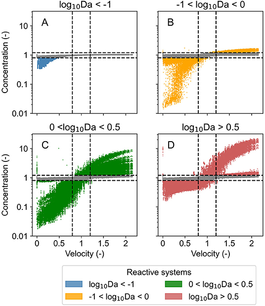
Figure 2. Concentration of chemical species belonging to identified categories of reaction regimes in all investigated domains normalized by that in steady state conditions with changing normalized velocity in corresponding domain (velocity normalized by that in steady state conditions) over the entire simulation period of 15 years for the three investigated time series (T1, T2, and T5). Points are colored when the change in concentration is 20% or higher, otherwise points are gray. Dashed black lines mark a change of 20% in normalized concentration and in normalized velocity. (A) Displays data for transport dominant regimes, (B) for transport influenced regimes, (C) for reaction influenced regimes, and (D) for reaction dominant regimes.
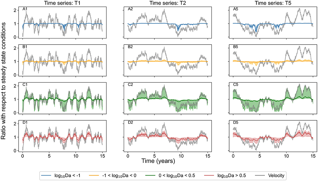
Figure 3. Median concentration of chemical species belonging to identified categories of reaction regimes in all investigated domains bound by 25 and 75% quartile ranges (red for reaction dominant regimes where log10Da > 0.5, green for regimes where, 0 < log10Da < 0.5, orange for regimes with −1 < log10Da < 0 and blue for reaction-limited regimes with log10Da < −1) over the entire simulation period of 15 years for the three investigated time series (T1, T2, and T5). Velocity normalized by that in steady state conditions is indicated by gray solid line. (A1,A2,A5) Display data for transport dominant regimes in three scenarios (time series T1, T2, and T5) respectively. (B1,B2,B5) Display data for transport influenced regimes in time series T1, T2, and T5 respectively. (C1,C2,C5) Display data for reaction influenced regimes in time series T1, T2, and T5 respectively. (D1,D2,D5) Display data for reaction dominant regimes in time series T1, T2, and T5 respectively.
The contribution of different fractions of microbial species also varied with temporally dynamic forcing. In all flow regimes, the ratio of active to dormant species increased with increasing velocity. The increase in the ratio was attributable to both, increasing active and decreasing dormant species with increasing velocity. The ratio of immobile and mobile species also increased with increasing velocity, but attributable only to decreasing mobile species in the domain (Figure 4). The shifting contribution of each microbial sub-population is presented in Supplementary Figure 14.
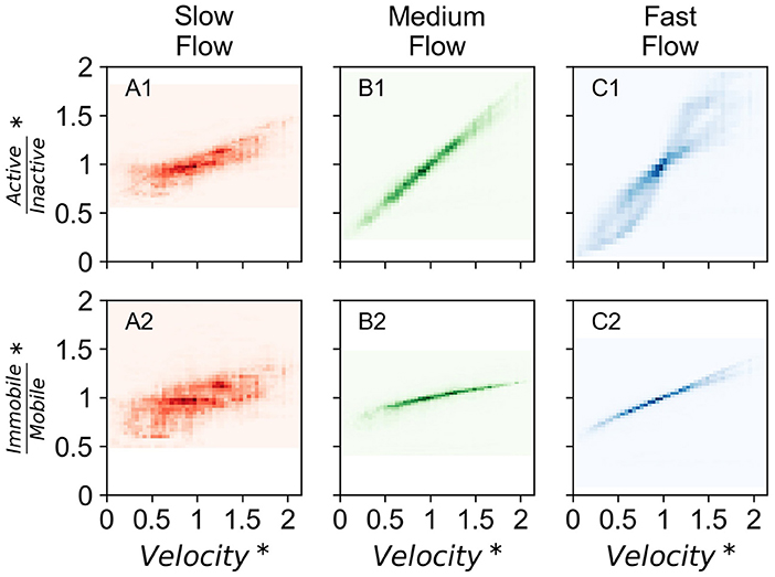
Figure 4. Density plot of contribution of microbial subpopulations in all investigated domains normalized by that in steady state conditions with normalized velocity in corresponding domain (velocity normalized by that in steady state conditions) over the entire simulation period of 15 years for the three investigated time series (T1, T2, and T5). Darker colors indicate higher density of points. (A1) Displays ratio of active and inactive biomass and (A2) displays ratio of immobile and mobile biomass in the slow flow regime. (B1) Displays ratio of active and inactive biomass and (B2) displays ratio of immobile and mobile biomass in the medium flow regime. (C1) Displays ratio of active and inactive biomass and (C2) displays ratio of immobile and mobile biomass in the fast flow regime. *Data points are normalized by that in steady state conditions.
As described in Section Temporal variation in microbial biomass, normalized responsiveness indicates the degree of variation in the time series with respect to homogeneous steady state conditions.
Each chemical species responded differently to forcing based on the flow regime (Supplementary Figure 12). In Figure 5, we presented the normalized responsiveness in terms of the Damköhler number of the prevailing reaction regime (estimated in corresponding steady state conditions). Heterogeneous transport dominated domains were little affected by temporal dynamics, the responsiveness of temporally dynamic spatially homogeneous domains being slightly higher. For transport influenced systems and reaction influenced systems, spatio-temporal heterogeneities induced a normalized responsiveness of 6–7 (that is, the amplitude was 500–600% higher than in homogeneous domains). With residence time < ~30 days, the normalized responsiveness increased, in moderately heterogeneous domains, and then tended back toward that in homogeneous domains when residence time reduced to approximately a day. For reaction dominated systems, the normalized responsiveness also depended on the residence time. For residence time of ~1 day, there was limited impact of temporal dynamics. With residence time between 1 and 30 days, the responsiveness increased with increasing spatial heterogeneity, inducing a normalized responsiveness higher than 10.
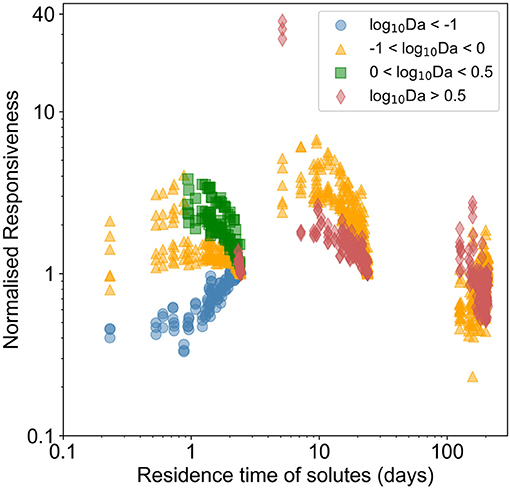
Figure 5. Normalized responsiveness of chemical species leaving the domain in temporally dynamic and spatially heterogeneous domains with respect to temporally dynamic homogeneous domain. The color varies with the prevalent reaction-flow regime (red for reaction dominant regimes where log10Da > 0.5, green for reaction influenced regimes where, 0 < log10Da < 0.5, orange for transport influenced regimes with −1 < log10Da < 0 and blue for transport dominated regimes with log10Da < −1). Normalized responsiveness close to 1 indicates that the temporal dynamics induced in a spatially heterogeneous domain is similar to those induced in the corresponding homogeneous domain.
For all microbial species highest normalized responsiveness values were ~1. We observed that the normalized responsiveness of all microbial species in all flow regimes, except for aerobes in the slow and medium flow regimes, reduced with increasing spatio-temporal heterogeneity. Figure 6 presents the normalized responsiveness of the active biomass in these heterogeneous domains normalized by that of the homogeneous domain.
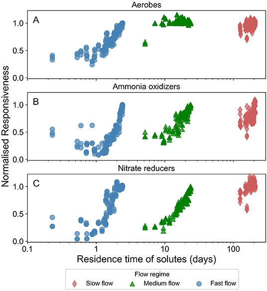
Figure 6. Normalized responsiveness of concentration of active fraction of biomass in the domain in response to temporal dynamics in the forcing (changing groundwater head at the inlet of the domain). The color varies with the prevalent flow regime (red for slow flow, green for medium flow, and blue for fast flow regimes). Normalized responsiveness close to 1 indicates that the temporal dynamics induced in a spatially heterogeneous domain is similar to those induced in the corresponding homogeneous domain. (A) Displays the data for active aerobic degraders (aerobes), (B) for active ammonia oxidizers, and (C) for active nitrate reducers.
The chemical species were moderately to strongly correlated with the forcing in medium and fast flow regimes. In the slow flow regime, DOC and DO had weak to moderately positive correlation. In contrast, TOC and nitrogen had weak to moderately negative correlation (Supplementary Figure 8).
The active microbial species in the medium flow regime were moderately to strongly correlated with the forcing. All the microbial species (except mobile aerobic degraders) were also similarly correlated with the forcing in the slow flow regime. Mobile aerobic degraders, on the other hand, were negatively correlated with the forcing. Lastly, all the microbial species (except aerobic degraders) were negatively correlated with the forcing in the fast flow regime. The immobile aerobic degraders were positively correlated with the forcing (Supplementary Figure 9).
We traced the variation in the microbial and physiochemical quality of the groundwater back to temporally dynamic forcing (changes in groundwater head in our case). A high backward traceability indicated that the impact of changes in forcing lasted a substantial amount of time. We contextualized backward traceability of the reactive domains with the memory of the temporally dynamic forcing (Table 2) by taking the ratio of the two.
The backward traceability varied from 0 days (in buffered slow flow regimes, for TOC in relatively homogeneous domains, and for nitrogen in selected transport dominated fast flow regimes) to up to 245 days (nitrate in medium flow regime in T5). In the fast flow regime, the backward traceability increased with heterogeneity and then decreased in high spatial heterogeneity scenarios for DOC, TOC, and DO (Supplementary Figure 10). In the medium flow regime, the backward traceability increased with spatial heterogeneity for all chemical species except for DO, for which it remained constant independent of spatial heterogeneity. The backward traceability of chemical species could not be evaluated in the slow flow regime as the correlation with the forcing was weak to moderate (Supplementary Figure 8). This means that any fluctuation in the concentration profile of the flux averaged concentrations of mobile species at the outlet of the domain is not attributable to a change in the forcing in the slow flow regime.
The backward traceability for active microbial biomass varied from 0 days (ammonia oxidizers, nitrate reducers and mobile aerobes in the fast flow regime) to ~280 days (immobile active ammonia oxidizers in slow flow regime in T5).
The backward traceability of the microbial species biomass in the slow flow regime was the highest (active immobile aerobes, ammonia oxidizers and nitrate reducers), followed by that in the medium flow regime and the fast flow regime (Supplementary Figure 11). Except for nitrate reducers, the backward traceability remained independent of the spatial heterogeneity in the domain. Among the nitrate reducers, the backward traceability reduced with increasing spatial heterogeneity in the medium flow regime only. The backward traceability for nitrate reducers in the slow flow and fast flow regimes also remained independent of spatial heterogeneity.
The response of nutrient cycling and microbial biomass to temporal dynamics in the forcing involved a detailed analysis of flow regime, spatial heterogeneity, and the intensity of temporal dynamics in the forcing. We observed that the concentration of chemical species leaving the domain varied over time, although the aggregated removal of the chemical species of the entire simulation period was the same as that in steady state conditions. We also observed that the biomass of the microbial species, the relative contribution of different fractions of microbial species in the domain varied over time. This is analogous to real-time data collected during long term environmental monitoring studies where varying groundwater head in monitoring wells is linked with varying physicochemical characteristics of groundwater (McGuire et al., 2000; Van Der Hoven et al., 2005). The predictability of the response of the system to temporal dynamics is confounded by both uncertainties in the flow regime and spatial heterogeneity. Here we shed light on their individual contributions and the consequences for modeling predictions.
As described in the Methods section, we explore a wide range of physically plausible scenarios of spatially heterogeneous domains and temporally dynamic scenarios. We varied the conductivity spatially in the domain to induce spatial heterogeneity. However, subsurface systems are spatially heterogeneous given variation in other properties as well, including porosity, surface properties of the matrix, and storativity. We did not explore variation in any other properties to induce spatial heterogeneity in the domain. It must be noted, though, that the explored scenarios of spatially distributed conductivity induced a reduction in breakthrough time as high as 80% of that in homogeneous scenarios. Given that breakthrough time is a suitable indicator of changing biogeochemical potential of most spatially heterogeneous reactive systems (Sanz-Prat et al., 2015, 2016; Khurana et al., 2022), we deemed this sufficient to derive uncertainty due to spatial heterogeneities in the domain. We expect that further studies exploring the impact of the above-mentioned properties of the domain to add to our findings.
Similar to spatially heterogeneous scenarios, we focused on developing temporal dynamics scenarios that would be comparable to steady state conditions. This assumes that long-term average conditions in the subsurface are stable. However, groundwater table is expected to drop in regions where it is used for irrigation (Huang et al., 2015), while it is expected to increase in regions with surface water irrigation or permafrost melt (Bense et al., 2009; Huang et al., 2015; Pholkern et al., 2018). We detail the implications of this further in the following sections.
Lastly, a major source of uncertainty is parametrization of the reaction network [as also described in the Introduction (Nitzsche et al., 2000)]. We sought to mitigate the uncertainty due to this on multiple levels. First, we coupled the same process network with the same parameters in all the scenarios (homogeneous and heterogeneous domains, in both steady state conditions and temporally dynamic hydrological settings). Second, we considered the homogeneous domains and steady state conditions as the base case. Recall, for example, that we normalized the responsiveness of spatially heterogeneous domains with that of homogeneous domains. Lastly, the characterization of subsurficial reactive systems may be done based on a dimensionless number (Da). This can be relatively easily estimated based on field data and its use mitigates the importance of accurate parameterization when predicting a system's response to changing forcing or domain characteristics. Thus, we can confidently explore the implications of the results of this study with respect to uncertainty induced by spatio-temporal heterogeneities.
This study explored biomass dynamics and nutrient cycling thereof in domains exhibiting spatio-temporal heterogeneities. Depending on the reaction and flow regime in the system, and temporal dynamics of the forcing, we can estimate the predictive uncertainty of chemical discharge from a domain caused by the associated spatio-temporal heterogeneities. The uncertainty bounds are therefore a good measure for the error that would result from neglecting them.
It is worthwhile to note that there was no substantial impact of temporal dynamics on removal of chemical species or the distribution of microbial species into various fractions when aggregated over the entire simulation period. Even for the exceptional case of nitrate in fast flow, the aggregated impact was marginal, since the observed large increase (~200%) in nitrate removal was with respect to very low removal in the steady state homogeneous domain; the removal increased from 1.1 to 2.7%. Thus, the relevance of uncertainty quantification in modeling studies must be examined with the research objective in mind. If we are interested in aggregated behaviors of the system over long periods, then the impact of sub-scale temporal dynamics is small and the system can be well-represented with a steady state model of the same residence time, akin to biogeochemical stationarity discussed by Basu et al. (2010) for above surface systems. The link between average behavior of subsurficial reactive systems with travel time has also been established (Sanz-Prat et al., 2015). Thus, aggregated removal of chemical species of the system is linked with the travel time of the system at the temporal scale of interest/in question. For example, if the travel time in a system increases over the time scale of interest, say due to lowering water table and decreasing hydraulic gradient, then we expect the aggregated removal of the chemical species in the system to increase, resulting in lower chemical discharge from the domain. At the same time, sub-scale temporal dynamics in chemical discharge can be characterized based on Damköhler number as in Khurana et al. (2022), whereby neglecting spatial heterogeneity alone may result in prediction errors from −60 to +500%. Transport dominated heterogeneous systems showed limited impact to temporal dynamics; most of which was attributable to the reduction of nitrate in unusually low flow conditions when velocity reduced to <50% of that in steady state conditions. Furthermore, the response of temporally dynamic spatially homogeneous domains was higher than that of heterogeneous domains. In other words, spatial heterogeneity dampened the impact of temporal dynamics on the reactive system. Temporal dynamics are therefore important in only unusually low flow conditions. Unusual here means that the average residence time is less than half of that in a corresponding homogeneous domain, caused by the strong heterogeneity, and at time points when the flow rate is also less than half of that in steady state conditions.
For transport or reaction influenced systems, spatio-temporal heterogeneities induce a normalized responsiveness of 6–7 (that is, moderately heterogeneous domains respond more than homogeneous domains by 500–600%). At the same time, high spatially heterogeneous domains respond the same as homogeneous domains. Thus, predictive uncertainty associated with temporal dynamics was adequately captured by homogeneous domains in high heterogeneity scenarios. However, in moderately heterogeneous domains, both spatial heterogeneity and temporal dynamics lead to strong deviations from the homogeneous cases and therefore heterogeneity needs to be accounted for when modeling these systems.
For reaction dominated regimes, the amplitude depended on the average residence time as well. When residence time was short (approximately a day), there was limited impact of temporal dynamics on the system. On the other hand, in medium flow systems, when residence time was higher than a fortnight, spatial heterogeneity accentuated the impact of temporal dynamics on the amplitude of the system, and the third quartile could be as high as twice the steady state conditions. Thus, spatio-temporal heterogeneities may not be neglected in these systems.
In general, the high responsiveness of the systems in the study was due to DO, nitrate and DOC traveling through the preferential flow paths in spatially heterogeneous domains. This behavior and extent of impact is consistent with previous studies. Gwo et al. (1996) proposed that 64% of variation in fluxes is attributable to spatial heterogeneity (hydraulic conductivity and anisotropy) and temporal dynamics (rainfall intensity). Van Der Hoven et al. (2005) observed even higher dynamics with a variation of DO over 2 orders of magnitude at their site. Rein et al. (2009) also observed that temporal variation in groundwater flow conditions resulted in variation of contaminant concentration (as high as the steady state/average concentration). More recently, Küsel et al. (2016) discussed variation of chemical species (such as DOC, DO, nitrate) by a factor of 3–4, both in space and in time. While a direct comparison between these previous studies and our results is ill advised considering differences in flow regimes, conceptual model, and site settings, it is worth to note that we observe variation over similar orders of magnitude and even higher since we considered a larger range of spatio-temporal variations.
To conclude, we estimated bounds of predictive uncertainty based on easily estimable field indicators (Da, travel time). Neglecting spatio-temporal heterogeneities resulted in large predictive uncertainty depending on the reactive system of interest. In transport dominated systems, parametrization uncertainty was much higher than predictive uncertainty, which was predicted to be as high as median concentration of chemical of concern by Nitzsche et al. (2000). In reaction dominated systems, the predictive uncertainty could be comparable to parametrization uncertainty. Note also that for the reaction network and parameters used in this study any scenarios with flow rates lower than the presented slow flow regime would have been reaction dominated systems. In the transport influenced and reaction influenced systems, neglecting spatio-temporal heterogeneities resulted in higher predictive uncertainty compared to parametrization uncertainty.
In this work, we considered a wide variety of flow regimes, a comprehensive and detailed process network, homogeneous uniform flow conditions as the base case, and stochastically generated time series of the forcing, and dimensionless numbers that are used for capturing scaling effects. Thus, this work comprehensively encapsulates the predictive uncertainty relevant at the field and policy scale (Muniruzzaman and Pedretti, 2021).
The distribution of the biomass among the various types of species changed in the temporally dynamic regimes where flow velocity varied in time. This agrees with previous research that attribute species composition to difference in the flow regimes (Grösbacher et al., 2018), the maximum carrying capacity (the limited capacity of the domain to host immobile microbes) (Grösbacher et al., 2018) and spatial heterogeneity of a system (Or et al., 2007; Franklin et al., 2019, 2021; Khurana et al., 2022). Since the slow flow regime is already transport limited, the temporal variation in inactive species appears to be stochastic in nature, enhancing predictive uncertainty. With increasing advection, the microbial community composition tends to become deterministic and predictable (Stegen et al., 2016), mitigating predictive uncertainty using the approach presented in this work. Notably, the biomass in low flow zones of transport dominated systems is less sensitive to temporal dynamics because the biomass in low-flow zones may not be reached by fluctuations in advection. In contrast, locally mixed or diffusion dominated heterogeneous domains as well as homogeneous domains respond similarly to temporal dynamics. Spatial heterogeneity and long transport time scales thus enhance resilience of microbial community structure to disturbances (König et al., 2017, 2018; Yabusaki et al., 2017). Thus, the relevance of spatio-temporal heterogeneities (and uncertainty thereof) for geomicrobial community structure and nutrient cycling is dependent on travel time and dominant flow processes. Spatio-temporal heterogeneities are more relevant in transport dominated systems and may be neglected in reaction dominated (or transport limited) systems.
The fluctuation of microbial communities attributable to groundwater or surface inputs was also observed in other studies. For example, King et al. (2017) demonstrated that the relative contribution of bacterial species in an in-field bioreactor changes between dry periods (oxic conditions) and wet periods (sub-oxic) conditions. Benk et al. (2019) further demonstrated that changing input of DOM between dry and wet seasons influences bacterial community evolution in a pristine oligotrophic aquifer under minimal anthropogenic impact or disturbance. Lohmann et al. (2020) also then focused on the shift from aerobic to anaerobic ammonium oxidation between summer (dry conditions) and autumn (wet conditions) at the same site. We observed that change in relative abundance of active species in the microbial community or the change in microbial activity did not lead to an impact of the same magnitude on chemical discharge. For example, even though the contribution of active nitrate reducers decreased during low flow conditions in the medium flow regime, we observed that nitrate removal increased. This points to the low microbial activity in low-flow periods as discussed by Stegen et al. (2016). Even though nitrate reduction increased during these periods, the proliferation and activity of nitrate reducers decreased as microbial activity is limited by transport. In contrast, during high flow periods, even though the discharge of nitrate increased, the contribution of active nitrate reducers did not change from steady state conditions, while the contribution of inactive nitrate reducers decreased. This points to flushing of both microbes and chemical species due to high flow rates (Stegen et al., 2016). Temporal dynamics thus enable higher diversity in the subsurface microbiome by enabling mobility of microbial species in high flow periods (King et al., 2017).
Having estimated the predictive uncertainty associated with temporal dynamics in forcing on the mobile species signal leaving the domain and microbial biomass within the domain, we now consider the implications for sampling design. Low variation of mobile species at the outlet of the domain indicates that the temporal dynamics in the forcing are potentially buffered by the flow regime at the scale of the domain (Alewell et al., 2006). Alternatively, the corresponding chemical species is not affected by excessive flow rates induced in the domain, for example nitrogen in the fast flow regime. Since nitrogen removal was already marginal at steady state conditions in the fast flow regime (Khurana et al., 2022), higher flow rates do little to reduce the consumption further. In contrast, lower flow rates induced in heterogeneous domains in the fast flow regime provide an opportunity for nitrate reducers to thrive in anaerobic microsites in heterogeneous domains, thereby resulting in increased consumption of nitrogen with both temporal dynamics and spatial heterogeneity. Lohmann et al. (2020) observed similar shifts from aerobic metabolism (ammonia oxidation during dry periods) to anaerobic metabolism (nitrate reduction and anaerobic ammonia oxidation during wet periods) in functional diversity of microbial communities in groundwater. This is hypothesized as a potential effect of climate change driven changing surficial processes by Stegen et al. (2016) as well. Interestingly, the low flow zones provided buffer zones to these anaerobic microsites in domains with high flow rates, and therefore the response of these microbial species was lower compared to temporally dynamic regimes in lower average flow rates (see discussion above).
Tracing temporally dynamic mobile species poses an additional challenge. The time-lag analysis provided insight into the traceability of temporal dynamics of the system to forcing (Kim et al., 2019). The lag between the forcing of groundwater head and corresponding response in the domain and at the outlet of the domain varied as per the flow regime, as well as the microbial and chemical species of concern. Depending on the time scale of interest, the frequency of sampling, and the timing of sampling must be governed by occurrence of weather events as well as broader seasonal changes. While the response in dissolved chemical species signal may be immediate (shorter than observation frequency, and shorter than the traceability of the time series signal itself) in high spatio-temporal heterogeneity and high flow rate regimes, the response is induced later and lasts longer on microbial species in medium and slow flow regimes. Also, the traceability for microbial biomass in slow and medium flow regimes was in the same range as that of the traceability of the forcing and was largely not dependent on the residence time of the domain. Interestingly Hofmann et al. (2020) concluded that microbial communities present in the shallow subsurface respond to changing surficial inputs (with residence time of ~15 h, corresponding to fast flow regime in our study) over 170 days, which is in the same order of magnitude as the traceability observed in our study. It was also in the same order of magnitude of that observed by Zhou et al. (2012), even though their study was a transport dominated system at the field scale as opposed to the sub-meter scale of our study. Thus, we link traceability with the time scale of respective microbial growth kinetics. Microbial species with lower respiration and growth rates are slower to adapt to dynamic environmental conditions, and therefore display a large time lag (or high traceability). Microbial population distribution shifts are attributable to shifting hospitable conditions for high adaptable microbial species, and increased mobility for low adaptable microbial species (Sugiyama et al., 2018). Therefore, the time scale of temporal dynamics of environmental conditions and subsequent impact must be considered in relation to the time scale of microbial kinetics. If the time scale of changing forcing is short in comparison to the time scale of microbial kinetics, then the observable impact on microbial biomass is expected to be less. Regardless of these differences in the extent of the system response, the time series signal of dissolved chemical species and microbial biomass is linked with that of groundwater head, which is in turn linked with surficial events. Therefore, none of these analyses may be undertaken in isolation.
Computational costs, lack of detailed characterization of geological setting, lack of temporal resolution in field monitoring leads to modelers assuming steady state homogeneous conditions of a natural system. Field scale studies do not resolve sub-scale spatial heterogeneity, thus contributing to uncertainty with respect to both parametrization and predictive outcomes of modeling studies. The uncertainty induced due to lack of characterization of spatial heterogeneity is further exacerbated by neglecting temporal dynamics. Additionally, prediction of temporal dynamics is also increasingly uncertain in a changing climate scenario, and we are not yet equipped to estimate the uncertainty in microbial activity, and chemical discharge thereof from subsurface reactive systems.
While we are not able to completely do away with the uncertainty associated with reactive transport modeling, this study is a first attempt to capture the extent of uncertainty were we to neglect spatio-temporal heterogeneities in modeling studies. With accurate site characterization, and contextualizing temporal dynamics, we can now assist in field sampling design to correlate field data with dynamics in forcing. With this, we aimed to reduce predictive uncertainty in modeling studies.
We explicitly accounted for both spatial and temporal heterogeneities and combined this with a comprehensive biogeochemical reaction network to estimate associated uncertainty. We captured a wide range of spatially heterogeneous scenarios, temporally dynamic regimes, flow regimes, four distinct microbial functional groups, to comprehensively propose the bounds of predictive uncertainty associated with spatio-temporal heterogeneities. We identified four (4) types of reactive systems: Transport dominated, transport influenced, reaction influenced, and reaction dominated, similar to that used in Khurana et al. (2022), based on the travel time and the logarithm of Damköhler number (log10Da) to categorize system response to spatio-temporal heterogeneities.
We found that both spatial and temporal heterogeneity impact biomass distribution and nutrient cycling to varying degrees (as high as 20 times that of average or steady state conditions), resulting in uncertainty in prediction of reactive transport models. We concluded that spatial heterogeneity has a higher bearing than temporal dynamics on nutrient cycling in extremely high spatio-temporal heterogeneous scenarios. In systems with high spatial heterogeneity or preferential flow paths, the aerobic conditions vary dramatically with forcing, but the appearance of anaerobic microsites leading to higher consumption of nitrate may only appear in extremely low flow periods. These conditions may be rare historically but are expected to occur with higher frequency with climate change driven processes (Stegen et al., 2016).
In cases of moderate spatially heterogeneous domains, temporal dynamics play a larger role in nutrient cycling. Furthermore, we concluded that temporal dynamics have a longer lasting impact on microbial community structure and corresponding redox conditions in heterogeneous subsurface domains (characterized by low variance domains in medium to slow flow regimes) such as alluvial sediments close to hyporheic zones with increased matter exchange between the surface and the subsurface.
This study provided a comprehensive estimate of predictive uncertainty if spatio-temporal heterogeneities were to be neglected. While predictive uncertainty could be as high as 10–20 times that of homogeneous steady state conditions depending on the reactive system of interest, neglecting temporal dynamics alone resulted in predictive uncertainty as well with the interquartile range being 50% lower to 100% higher than that in average or steady state conditions.
The processed datasets and results are available in an online repository (Khurana, 2021).
SK conceptualized the reaction network, defined the simulation scenarios, executed the simulations, analyzed the results, and drafted the manuscript. FH, AH, and MT provided guidance and technical support. MT defined and supervised the study. All authors contributed to the interpretation of the results and editing the manuscript. All authors contributed to the article and approved the submitted version.
This study was part of the Collaborative Research Center of the Friedrich Schiller University Jena, funded by the Deutsche Forschungsgemeinschaft (DFG, German Research Foundation)—SFB 1076—Project Number 218627073.
The authors declare that the research was conducted in the absence of any commercial or financial relationships that could be construed as a potential conflict of interest.
All claims expressed in this article are solely those of the authors and do not necessarily represent those of their affiliated organizations, or those of the publisher, the editors and the reviewers. Any product that may be evaluated in this article, or claim that may be made by its manufacturer, is not guaranteed or endorsed by the publisher.
The Supplementary Material for this article can be found online at: https://www.frontiersin.org/articles/10.3389/frwa.2022.780297/full#supplementary-material
Aguilera, D. R., Jourabchi, P., Spiteri, C., and Regnier, P. (2005). A knowledge-based reactive transport approach for the simulation of biogeochemical dynamics in Earth systems. Geochem. Geophys. Geosyst. 6, Q07012. doi: 10.1029/2004GC000899
Alewell, C., Paul, S., Lischeid, G., Küsel, K., and Gehre, M. (2006). Characterizing the redox status in three different forested wetlands with geochemical data. Environ. Sci. Technol. 40, 7609–7615. doi: 10.1021/es061018y
Basu, N. B., Destouni, G., Jawitz, J. W., Thompson, S. E., Loukinova, N. V., Darracq, A., et al. (2010). Nutrient loads exported from managed catchments reveal emergent biogeochemical stationarity. Geophys. Res. Lett. 37, L23404. doi: 10.1029/2010GL045168
Benk, S. A., Yan, L., Lehmann, R., Roth, V.-N., Schwab, V. F., Totsche, K. U., et al. (2019). Fueling diversity in the subsurface: composition and age of dissolved organic matter in the critical zone. Front. Earth Sci. 7, 296. doi: 10.3389/feart.2019.00296
Bense, V. F., Ferguson, G., and Kooi, H. (2009). Evolution of shallow groundwater flow systems in areas of degrading permafrost. Geophys. Res. Lett. 36, L22401. doi: 10.1029/2009GL039225
Berkowitz, B.. (2002). Characterizing flow and transport in fractured geological media: a review. Adv. Water Resourc. 25, 861–884. doi: 10.1016/S0309-1708(02)00042-8
Berkowitz, B., Dror, I., Hansen, S. K., and Scher, H. (2016). Measurements and models of reactive transport in geological media. Rev. Geophys. 54, 930–986. doi: 10.1002/2016RG000524
Bhattacharyya, A., Campbell, A. N., Tfaily, M. M., Lin, Y., Kukkadapu, R. K., Silver, W. L., et al. (2018). Redox fluctuations control the coupled cycling of iron and carbon in tropical forest soils. Environ. Sci. Technol. 52, 14129–14139. doi: 10.1021/acs.est.8b03408
Cai, W., Borlace, S., Lengaigne, M., Van Rensch, P., Collins, M., Vecchi, G., et al. (2014). Increasing frequency of extreme El Niño events due to greenhouse warming. Nat. Clim. Chang. 4, 111–116. doi: 10.1038/nclimate2100
Centler, F., Hesse, F., and Thullner, M. (2013). Estimating pathway-specific contributions to biodegradation in aquifers based on dual isotope analysis: theoretical analysis and reactive transport simulations. J. Contam. Hydrol. 152, 97–116. doi: 10.1016/j.jconhyd.2013.06.009
Centler, F., Shao, H., De Biase, C., Park, C. H., Regnier, P., Kolditz, O., et al. (2010). GeoSysBRNS-A flexible multidimensional reactive transport model for simulating biogeochemical subsurface processes. Comput. Geosci. 36, 397–405. doi: 10.1016/j.cageo.2009.06.009
Chakrawal, A., Herrmann, A. M., Koestel, J., Jarsj,ö, J., Nunan, N., Kätterer, T., et al. (2020). Dynamic upscaling of decomposition kinetics for carbon cycling models. Geosci. Model Dev. 13, 1399–1429. doi: 10.5194/gmd-13-1399-2020
Cohen, J., Screen, J. A., Furtado, J. C., Barlow, M., Whittleston, D., Coumou, D., et al. (2014). Recent arctic amplification and extreme mid-latitude weather. Nat. Geosci. 7, 627–637. doi: 10.1038/ngeo2234
Danczak, R. E., Sawyer, A. H., Williams, K. H., Stegen, J. C., Hobson, C., and Wilkins, M. J. (2016). Seasonal hyporheic dynamics control coupled microbiology and geochemistry in Colorado river sediments. J. Geophys. Res. Biogeosci. 121, 2976–2987. doi: 10.1002/2016JG003527
de Marsily, G., Delay, F., Gonçalvès, J., Renard, P., Teles, V., and Violette, S. (2005). Dealing with spatial heterogeneity. Hydrogeol. J. 13, 161–183. doi: 10.1007/s10040-004-0432-3
Duffy, C. J., and Gelhar, L. W. (1985). A frequency domain approach to water quality modeling in groundwater: theory. Water Resourc. Res. 21, 1175–1184. doi: 10.1029/WR021i008p01175
Easterling, D. R., Meehl, G. A., Parmesan, C., Changnon, S. A., Karl, T. R., and Mearns, L. O. (2000). Climate extremes: observations, modeling, and impacts. Science 289, 2068–2074. doi: 10.1126/science.289.5487.2068
Febria, C. M., Fulthorpe, R. R., and Williams, D. D. (2010). Characterizing seasonal changes in physicochemistry and bacterial community composition in hyporheic sediments. Hydrobiologia 647, 113–126. doi: 10.1007/s10750-009-9882-x
Franklin, S., Kravchenko, A., Vargas, R., Vasilas, B., Fuhrmann, J. J., and Jin, Y. (2021). The unexplored role of preferential flow in soil carbon dynamics. Soil Biol. Biochem. 161, 108398. doi: 10.1016/j.soilbio.2021.108398
Franklin, S., Vasilas, B., and Jin, Y. (2019). More than meets the dye: evaluating preferential flow paths as microbial hotspots. Vadose Zone J. 18, 190024. doi: 10.2136/vzj2019.03.0024
Grösbacher, M., Eckert, D., Cirpka, O. A., and Griebler, C. (2018). Contaminant concentration versus flow velocity: drivers of biodegradation and microbial growth in groundwater model systems. Biodegradation 29, 211–232. doi: 10.1007/s10532-018-9824-2
Gwo, J. P., Toran, L. E., Morris, M. D., and Wilson, G. V. (1996). Subsurface stormflow modeling with sensitivity analysis using a latin-hypercube sampling technique. Ground Water 34, 811–818. doi: 10.1111/j.1745-6584.1996.tb02075.x
Hofmann, R., Uhl, J., Hertkorn, N., and Griebler, C. (2020). Linkage between dissolved organic matter transformation, bacterial carbon production, and diversity in a shallow oligotrophic aquifer: results from flow-through sediment microcosm experiments. Front. Microbiol. 11, 543567. doi: 10.3389/fmicb.2020.543567
Huang, Y., Salama, M. S., Krol, M. S., Su, Z., Hoekstra, A. Y., Zeng, Y., et al. (2015). Estimation of human-induced changes in terrestrial water storage through integration of GRACE satellite detection and hydrological modeling: a case study of the Yangtze River basin. Water Resour. Res. 51, 8494–8516. doi: 10.1002/2015WR016923
Jing, M., Heße, F., Kumar, R., Wang, W., Fischer, T., Walther, M., et al. (2018). Improved regional-scale groundwater representation by the coupling of the mesoscale Hydrologic Model (mHM v5.7) to the groundwater model OpenGeoSys (OGS). Geosci. Model Dev. 11, 1989–2007. doi: 10.5194/gmd-11-1989-2018
Khatri, N., and Tyagi, S. (2015). Influences of natural and anthropogenic factors on surface and groundwater quality in rural and urban areas. Front. Life Sci. 8, 23–39. doi: 10.1080/21553769.2014.933716
Khurana, S.. (2021). Temporal Uncertainty of Microbial Nutrient Cycling in Groundwater [Python]. Zenodo [code]. doi: 10.5281/zenodo.5516917
Khurana, S., Heße, F., Hildebrandt, A., and Thullner, M. (2022). Predicting the impact of spatial heterogeneity on microbial redox dynamics and nutrient cycling in the subsurface. Biogeosci. 19, 665–688. doi: 10.5194/bg-19-665-2022
Kim, K. H., Michael, H. A., Field, E. K., and Ullman, W. J. (2019). Hydrologic shifts create complex transient distributions of particulate organic carbon and biogeochemical responses in beach aquifers. J. Geophys. Res. Biogeosci. 124, 3024–3038. doi: 10.1029/2019JG005114
King, A. J., Preheim, S. P., Bailey, K. L., Robeson, M. S., Roy Chowdhury, T., Crable, B. R., et al. (2017). Temporal dynamics of in-field bioreactor populations reflect the groundwater system and respond predictably to perturbation. Environ. Sci. Technol. 51, 2879–2889. doi: 10.1021/acs.est.6b04751
Kohlhepp, B., Lehmann, R., Seeber, P., Küsel, K., Trumbore, S. E., and Totsche, K. U. (2017). Aquifer configuration and geostructural links control the groundwater quality in thin-bedded carbonate–siliciclastic alternations of the Hainich CZE, central Germany. Hydrol. Earth Syst. Sci. 21, 6091–6116. doi: 10.5194/hess-21-6091-2017
Köhne, J. M., Köhne, S., and Šimunek, J. (2009). A review of model applications for structured soils: a) water flow and tracer transport. J. Contam. Hydrol. 104, 4–35. doi: 10.1016/j.jconhyd.2008.10.002
Kolditz, O., Bauer, S., Bilke, L., Böttcher, N., Delfs, J. O., Fischer, T., et al. (2012). OpenGeoSys: an open-source initiative for numerical simulation of thermo-hydro-mechanical/chemical (THM/C) processes in porous media. Environ. Earth Sci. 67, 589–599. doi: 10.1007/s12665-012-1546-x
Kolehmainen, R. E., Tiirola, M., and Puhakka, J. A. (2008). Spatial and temporal changes in actinobacterial dominance in experimental artificial groundwater recharge. Water Res. 42, 4525–4537. doi: 10.1016/j.watres.2008.07.039
König, S., Worrich, A., Banitz, T., Centler, F., Harms, H., Kästner, M., et al. (2018). Spatiotemporal disturbance characteristics determine functional stability and collapse risk of simulated microbial ecosystems. Sci. Rep. 8, 9488. doi: 10.1038/s41598-018-27785-4
König, S., Worrich, A., Centler, F., Wick, L. Y., Miltner, A., Kästner, M., et al. (2017). Modelling functional resilience of microbial ecosystems: analysis of governing processes. Environ. Model. Softw. 89, 31–39. doi: 10.1016/j.envsoft.2016.11.025
Küsel, K., Totsche, K. U., Trumbore, S. E., Lehmann, R., Steinhäuser, C., and Herrmann, M. (2016). How deep can surface signals be traced in the critical zone? Merging biodiversity with biogeochemistry research in a central German muschelkalk landscape. Front. Earth Sci. 4:32. doi: 10.3389/feart.2016.00032
Lambin, E. F., Geist, H. J., and Lepers, E. (2003). Dynamics of land-use and land-cover change in tropical regions. Annu. Rev. Environ. Resour. 28, 241. doi: 10.1146/annurev.energy.28.050302.105459
Leavitt, J. J., Howe, K. J., and Cabaniss, S. E. (2011). Equilibrium modeling of U(VI) speciation in high carbonate groundwaters: model error and propagation of uncertainty. Appl. Geochem. 26, 2019–2026. doi: 10.1016/j.apgeochem.2011.06.031
Lehmann, K., Lehmann, R., and Totsche, K. U. (2021). Event-driven dynamics of the total mobile inventory in undisturbed soil account for significant fluxes of particulate organic carbon. Sci. Total Environ. 756, 143774. doi: 10.1016/j.scitotenv.2020.143774
Lohmann, P., Benk, S., Gleixner, G., Potthast, K., Michalzik, B., Jehmlich, N., et al. (2020). Seasonal patterns of dominant microbes involved in central nutrient cycles in the subsurface. Microorganisms 8, 1694. doi: 10.3390/microorganisms8111694
McGuire, J. T., Smith, E. W., Long, D. T., Hyndman, D. W., Haack, S. K., Klug, M. J., et al. (2000). Temporal variations in parameters reflecting terminal-electron-accepting processes in an aquifer contaminated with waste fuel and chlorinated solvents. Chem. Geol. 169, 471–485. doi: 10.1016/S0009-2541(00)00223-0
Meng, L., Zuo, R., Wang, J. S., Li, Q., Du, C., Liu, X., et al. (2021). Response of the redox species and indigenous microbial community to seasonal groundwater fluctuation from a typical riverbank filtration site in Northeast China. Ecol. Eng. 159, 106099. doi: 10.1016/j.ecoleng.2020.106099
Moore, D. S., Notz, W. I., and Flinger, M. A. (2013). The Basic Practice of Statistics. New York, NY: W.H. Freeman and Company.
Moore-Kucera, J., and Dick, R. P. (2008). PLFA profiling of microbial community structure and seasonal shifts in soils of a Douglas-fir chronosequence. Microb. Ecol. 55, 500–511. doi: 10.1007/s00248-007-9295-1
Müller, S., Schüler, L., Zech, A., and Heße, F. (2021a). GSTools v1.3: a toolbox for geostatistical modelling in Python. Geosci. Model Dev. Discus. 2021, 1–33. doi: 10.5194/gmd-2021-301
Müller, S., Zech, A., and Heße, F. (2021b). ogs5py: a python-API for the OpenGeoSys 5 scientific modeling package. Groundwater 59, 117–122. doi: 10.1111/gwat.13017
Muniruzzaman, M., and Pedretti, D. (2021). Mechanistic models supporting uncertainty quantification of water quality predictions in heterogeneous mining waste rocks: a review. Stochast. Environ. Res. Risk Assess. 35, 985–1001. doi: 10.1007/s00477-020-01884-z
Nitzsche, O., Meinrath, G., and Merkel, B. (2000). Database uncertainty as a limiting factor in reactive transport prognosis. J. Contam. Hydrol. 44, 223–237. doi: 10.1016/S0169-7722(00)00106-6
Okkonen, J., Jyrkama, M., and Kløve, B. (2010). A conceptual approach for assessing the impact of climate change on groundwater and related surface waters in cold regions (Finland). Hydrogeol. J. 18, 429–439. doi: 10.1007/s10040-009-0529-9
Or, D., Smets, B. F., Wraith, J. M., Dechesne, A., and Friedman, S. P. (2007). Physical constraints affecting bacterial habitats and activity in unsaturated porous media—a review. Adv. Water Resourc. 30, 1505–1527. doi: 10.1016/j.advwatres.2006.05.025
Pett-Ridge, J., Petersen, D. G., Nuccio, E., and Firestone, M. K. (2013). Influence of oxic/anoxic fluctuations on ammonia oxidizers and nitrification potential in a wet tropical soil. FEMS Microbiol. Ecol. 85, 179–194. doi: 10.1111/1574-6941.12111
Pholkern, K., Saraphirom, P., and Srisuk, K. (2018). Potential impact of climate change on groundwater resources in the Central Huai Luang Basin, Northeast Thailand. Sci. Total Environ. 633, 1518–1535. doi: 10.1016/j.scitotenv.2018.03.300
Pittroff, M., Frei, S., and Gilfedder, B. S. (2017). Quantifying nitrate and oxygen reduction rates in the hyporheic zone using 222Rn to upscale biogeochemical turnover in rivers. Water Resour. Res. 53, 563–579. doi: 10.1002/2016WR018917
Rein, A., Bauer, S., Dietrich, P., and Beyer, C. (2009). Influence of temporally variable groundwater flow conditions on point measurements and contaminant mass flux estimations. J. Contam. Hydrol. 108, 118–133. doi: 10.1016/j.jconhyd.2009.06.005
Rezanezhad, F., Couture, R. M., Kovac, R., O'Connell, D., and Van Cappellen, P. (2014). Water table fluctuations and soil biogeochemistry: an experimental approach using an automated soil column system. J. Hydrol. 509, 245–256. doi: 10.1016/j.jhydrol.2013.11.036
Ritschel, T., and Totsche, K. U. (2016). Closed-flow column experiments: a numerical sensitivity analysis of reactive transport and parameter uncertainty. Water Resour. Res. 52, 6094–6110. doi: 10.1002/2015WR018388
Rudolf von Rohr, M., Hering, J. G., Kohler, H. P. E., and Von Gunten, U. (2014). Column studies to assess the effects of climate variables on redox processes during riverbank filtration. Water Res. 61, 263–275. doi: 10.1016/j.watres.2014.05.018
Sanz-Prat, A., Lu, C., Finkel, M., and Cirpka, O. A. (2015). On the validity of travel-time based nonlinear bioreactive transport models in steady-state flow. J. Contam. Hydrol. 175–176, 26–43. doi: 10.1016/j.jconhyd.2015.02.003
Sanz-Prat, A., Lu, C., Finkel, M., and Cirpka, O. A. (2016). Using travel times to simulate multi-dimensional bioreactive transport in time-periodic flows. J. Contam. Hydrol. 187, 1–17. doi: 10.1016/j.jconhyd.2016.01.005
Sassen, D. S., Hubbard, S. S., Bea, S. A., Chen, J., Spycher, N., and Denham, M. E. (2012). Reactive facies: an approach for parameterizing field-scale reactive transport models using geophysical methods. Water Resour. Res. 48, W10526. doi: 10.1029/2011WR011047
Shi, X., Ye, M., Curtis, G. P., Miller, G. L., Meyer, P. D., Kohler, M., et al. (2014). Assessment of parametric uncertainty for groundwater reactive transport modeling. Water Resour. Res. 50, 4416–4439. doi: 10.1002/2013WR013755
Siebert, S., Burke, J., Faures, J. M., Frenken, K., Hoogeveen, J., Döll, P., et al. (2010). Groundwater use for irrigation – a global inventory. Hydrol. Earth Syst. Sci. 14, 1863–1880. doi: 10.5194/hess-14-1863-2010
Sinke, A. J. C., Dury, O., and Zobrist, J. (1998). Effects of a fluctuating water table: column study on redox dynamics and fate of some organic pollutants. J. Contam. Hydrol. 33, 231–246. doi: 10.1016/S0169-7722(98)00072-2
Stegen, J. C., Fredrickson, J. K., Wilkins, M. J., Konopka, A. E., Nelson, W. C., Arntzen, E. V., et al. (2016). Groundwater-surface water mixing shifts ecological assembly processes and stimulates organic carbon turnover. Nat. Commun. 7, 11237. doi: 10.1038/ncomms11237
Sugiyama, A., Masuda, S., Nagaosa, K., Tsujimura, M., and Kato, K. (2018). Tracking the direct impact of rainfall on groundwater at Mt. Fuji by multiple analyses including microbial DNA. Biogeosciences 15, 721–732. doi: 10.5194/bg-15-721-2018
Trenberth, K. E., Dai, A., Rasmussen, R. M., and Parsons, D. B. (2003). The changing character of precipitation. Bull. Am. Meteorol. Soc. 84, 1205–1217. doi: 10.1175/BAMS-84-9-1205
Trenberth, K. E., Dai, A., Van Der Schrier, G., Jones, P. D., Barichivich, J., Briffa, K. R., et al. (2014). Global warming and changes in drought. Nat. Clim. Chang. 4, 17–22. doi: 10.1038/nclimate2067
UNESCO and UN-Water (2020). The United Nations World Water Development Report 2020: Water and Climate Change. Paris: UNESCO.
Van Der Hoven, S. J., Solomon, D. K., and Moline, G. R. (2005). Natural spatial and temporal variations in groundwater chemistry in fractured, sedimentary rocks: scale and implications for solute transport. Appl. Geochem. 20, 861–873. doi: 10.1016/j.apgeochem.2004.11.013
van Rossum, G., and Drake, F. L. (2006). The Python Language Reference Manual (Version 3.2). Bristol: Network Theory Ltd.
Vidal-Gavilan, G., Carrey, R., Solanas, A., and Soler, A. (2014). Feeding strategies for groundwater enhanced biodenitrification in an alluvial aquifer: chemical, microbial and isotope assessment of a 1D flow-through experiment. Sci. Total Environ. 494–495, 241–251. doi: 10.1016/j.scitotenv.2014.06.100
Virtanen, P., Gommers, R., Oliphant, T. E., Haberland, M., Reddy, T., Cournapeau, D., et al. (2020). SciPy 1.0: fundamental algorithms for scientific computing in python. Nat. Methods 17, 261–272. doi: 10.1038/s41592-019-0686-2
World Water Assessment Programme (2009). The United Nations World Water Development Report 3: Water in a Changing World (Water in a Changing World). Paris: UNESCO; London: Earthscan.
Yabusaki, S. B., Wilkins, M. J., Fang, Y., Williams, K. H., Arora, B., Bargar, J., et al. (2017). Water table dynamics and biogeochemical cycling in a shallow, variably-saturated floodplain. Environ. Sci. Technol. 51, 3307–3317. doi: 10.1021/acs.est.6b04873
Yan, L., Hermans, S. M., Totsche, K. U., Lehmann, R., Herrmann, M., and Küsel, K. (2021). Groundwater bacterial communities evolve over time in response to recharge. Water Res. 201, 117290. doi: 10.1016/j.watres.2021.117290
Zhang, X., Ma, F., Yin, S., Wallace, C. D., Soltanian, M. R., Dai, Z., et al. (2021). Application of upscaling methods for fluid flow and mass transport in multi-scale heterogeneous media: a critical review. Appl. Energy 303, 117603. doi: 10.1016/j.apenergy.2021.117603
Zheng, T., Deng, Y., Wang, Y., Jiang, H., O'Loughlin, E. J., Flynn, T. M., et al. (2019). Seasonal microbial variation accounts for arsenic dynamics in shallow alluvial aquifer systems. J. Hazard. Mater. 367, 109–119. doi: 10.1016/j.jhazmat.2018.12.087
Keywords: reactive transport modeling, spatio-temporal heterogeneity, uncertainty, geomicrobial activity, nutrient export
Citation: Khurana S, Heße F, Hildebrandt A and Thullner M (2022) Should We Worry About Surficial Dynamics When Assessing Nutrient Cycling in the Groundwater? Front. Water 4:780297. doi: 10.3389/frwa.2022.780297
Received: 20 September 2021; Accepted: 10 February 2022;
Published: 24 March 2022.
Edited by:
Alberto Bellin, University of Trento, ItalyReviewed by:
Xiaofan Yang, Beijing Normal University, ChinaCopyright © 2022 Khurana, Heße, Hildebrandt and Thullner. This is an open-access article distributed under the terms of the Creative Commons Attribution License (CC BY). The use, distribution or reproduction in other forums is permitted, provided the original author(s) and the copyright owner(s) are credited and that the original publication in this journal is cited, in accordance with accepted academic practice. No use, distribution or reproduction is permitted which does not comply with these terms.
*Correspondence: Swamini Khurana, c3dhbWluaS5raHVyYW5hQGdtYWlsLmNvbQ==
Disclaimer: All claims expressed in this article are solely those of the authors and do not necessarily represent those of their affiliated organizations, or those of the publisher, the editors and the reviewers. Any product that may be evaluated in this article or claim that may be made by its manufacturer is not guaranteed or endorsed by the publisher.
Research integrity at Frontiers
Learn more about the work of our research integrity team to safeguard the quality of each article we publish.