 Anurag Verma
 Prabhakar Sharma
95% of researchers rate our articles as excellent or good
Learn more about the work of our research integrity team to safeguard the quality of each article we publish.
Find out more
ORIGINAL RESEARCH article
Front. Water , 07 January 2022
Sec. Water Resource Management
Volume 3 - 2021 | https://doi.org/10.3389/frwa.2021.802095
This article is part of the Research Topic Groundwater Salinity: Origin, Impact, and Potential Remedial Measures and Management Solutions View all 5 articles
Growing dependence on groundwater to fulfill the water demands has led to continuous depletion of groundwater levels and, consequently, poses the maintenance of optimum groundwater and management challenge. The region of South Bihar faces regular drought and flood situations, and due to the excessive pumping, the groundwater resources are declining. Rainwater harvesting has been recommended for the region; however, there are no hydrogeological studies concerning groundwater recharge. Aquifer storage and recovery (ASR) is a managed aquifer recharge technique to store excess water in the aquifer through borewells to meet the high-water demand in the dry season. Therefore, this paper presents the hydrogeological feasibility for possible ASR installations in shallow aquifers of South Bihar with the help of flowing fluid electrical conductivity (FFEC) logging. For modeling, the well logging data of two shallow borewells (16- and 47-m depth) at Rajgir, Nalanda, were used to obtain the transmissivity and thickness of the aquifers. The estimated transmissivities were 804 m2/day with an aquifer thickness of 5 m (in between 11 and 16 m) at Ajatshatru Residential Hall (ARH) well. They were 353 and 1,154 m2/day with the aquifer thicknesses of 6 m (in between 16 and 22 m) and 2 m (in between 45 and 47 m), respectively, at Nalanda University Campus (NUC) well. Despite the acceptable transmissivities at these sites, those aquifers may not be fruitful for the medium- to large-scale (more than 100-m3/day injection rate) ASR as the thickness of the aquifers is relatively small and may not efficiently store and withdraw a large amount of water. However, these aquifers can be adequate for small (up to 20-m3/day injection rate) ASR, for example, groundwater recharge using rooftop water. For medium- to large-scale ASR, deeper aquifers need to be further explored on these sites or aquifers with similar characteristics.
The increasing worldwide demand for water is caused by increasing irrigation demand, urbanization, industrialization, and climate change, which ultimately poses stress on groundwater resources (Bouwer, 2002; Elshall et al., 2020). Due to excessive groundwater pumping, which exceeds the natural recharge through rainfall or other forms of precipitations, the rivers or other water bodies and groundwater level have declined especially in the semi-arid and arid areas due to intensive irrigation (Rodell et al., 2009; Wada et al., 2014; Cotterman et al., 2018). In India, due to the monsoon (rainy season), there is a larger availability of surface water for a short time period than groundwater. However, surface water availability is not uniformly distributed in space and time, making it an unreliable source of water supply. In contrast, groundwater can be used with little or without treatment; therefore, groundwater is being extensively exploited for irrigation, industrial, and domestic usage (Suhag, 2016). Bihar is one of the poorest states of India; the economy is mainly dependent on agriculture, which is affected by both excess rainfall and drought. It is unique in terms of its water challenges, characterized by periodic episodes of devastating floods and droughts (Yaduvanshi et al., 2015). The current trend of declining annual rainfall with increasing heavy rainfall events had further worsened the situation (Guhathakurta et al., 2020). The situation will be grimmer under the warming climate and unsustainable economic growth as there is a noticeable decline in average rainfall, increase in heavy rainfall, and higher evaporative losses (Aadhar and Mishra, 2020; Guhathakurta et al., 2020). Roxy et al. (2017) had found out that during 1950–2015, there was a 10% decline in the average annual rainfall but an increase in the number of extreme rainfall (more than 50 mm in 24 h) events by 75% in central India. The rainwater harvesting schemes to recharge the groundwater can be an option to mitigate such situations (Central Ground Water Board., 2003; Dillon et al., 2019). Adoption of rainwater harvesting technology can help in mitigating the issue of waterlogging by storing excess water in aquifers and utilizing this stored water in dry seasons.
Managed aquifer recharge (MAR) is recently getting popular as a water conservation mechanism over water storage in conventional surface reservoirs due to its various advantages, such as less land requirements, less sedimentation, negligible evaporation losses, less chances of structural failure, and water contamination (Dillon et al., 2019). Aquifer storage and recovery (ASR) is a type of MAR method to store excess water in aquifers when the water demand is low and use them later when the demand is high (Pyne, 2005; Bandyopadhyay et al., 2021). In comparison with other recharge methods, ASR requires very less space over the ground surface, and it is one of the economical groundwater recharge methods (Sultana et al., 2015). Apart from storing the water in aquifers, ASR is also known for improving groundwater quality (Page et al., 2017; Vanderzalm et al., 2020).
According to Pyne (2005), understanding the thickness and hydraulic properties of the potential aquifers for storage and recovery plays an essential role in the success of ASR operations. For the feasibility assessment of ASR, transmissivity is an essential feature to be studied, and it can affect both the amount of injection and the storage of injected water in the periphery of ASR well (Maliva and Missimer, 2010). Brown et al. (2005) suggested the most feasible transmissivity range as 465 to 2,323 m2/day with a minimum aquifer thickness of 8 m for an efficient ASR system.
The geophysical logging information can be very valuable for ASR and other recharge mechanisms for assessing the feasibility by analyzing the high-resolution continuous data of aquifers, such as flow zones or conductive fractures, transmissivity, salinity, electric conductivity or resistivity, mixing zone of stored (or injected) water, native water, etc. (Maliva et al., 2009). In general, geophysical logging studies, such as natural gamma logs, flowmeter logs, temperature logs, and resistivity logs had been used for finding the potential aquifers for storage and for estimating the hydraulic characterization of flow zones (Petkewich et al., 2004; Maliva et al., 2009; Alqahtani et al., 2021; LaHaye et al., 2021). Electrical conductivity loggings were used to determine the exact location of injected water and the native-injected water interface after the storage period (Zuurbier et al., 2014, 2015). Several other geophysical logging methods are being used to determine the abovementioned features, but it can be determined more efficiently by a single logging method called flowing fluid electric conductivity (FFEC) logging (Tsang et al., 1990). Generally, FFEC logging is being used for deep borewell aquifer characterization (Tsang et al., 1990; Doughty et al., 2005, 2008, 2013; Sharma et al., 2016); however, it has also been applied in shallow bore wells (Evans, 1995; Paillet and Pedler, 1996; Karasaki et al., 2000; Collins and Bianchi, 2020). Compared with other available logging methods, FFEC logging is economical, simple to use, and can characterize multiple aquifer features (Tsang et al., 1990; Doughty et al., 2005, 2017; Collins and Bianchi, 2020).
This paper presents the application of FFEC logging method for the feasibility of low-cost ASR into the unconfined aquifer through detailed hydrogeological characterization of two shallow wells (16- and 47-m depth) situated at Rajgir, Bihar, India. Furthermore, the inflow strength of the natural groundwater flow, hydraulic conductivity, thickness, and the respective transmissivity of aquifers has been estimated using one-dimensional model (BORE II) and Darcy's law for these shallow wells.
The study area is situated in Rajgir, the southern part of Nalanda district of Bihar, India, as shown in Figure 1. These wells lie in the marginal alluvium unconfined aquifer bordering Rajgir Hills. The maximum elevation of Rajgir Hills is 338 m above the mean sea level (Central Ground Water Board., 2013). The crystalline rocks exposed in Rajgir Hills form the bedrock inclined toward the north consisting of phyllites and quartzites along with pegmatitic intrusions. The Precambrian crystalline in the area has undergone intense structural disturbances manifested in the form of multiple folding. Lithologically, this region has been characterized by clay layers and mixed layers of sand and gravel of different size grades in upper aquifers (Chakroborty and Chattopadhyay, 2001; Saha et al., 2010). Farther north of the study area, the region consists of four alluvial fills, starting with clay at the top, coarse sand to gravel at the base, as noticed within a depth of 100–120 m below ground level (bgl) (Central Ground Water Board., 2013). The groundwater is developed through wellbores and dug wells above the bedrock in this region, and the average groundwater level varies between 5 and 10 m bgl (Central Ground Water Board., 2013).
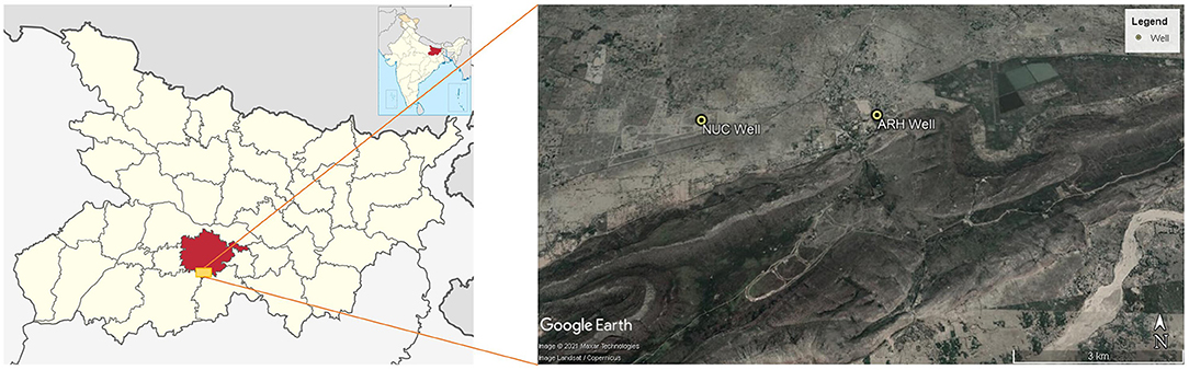
Figure 1. Location map (using Google Earth) showing well sites at the Nalanda University Campus (NUC) and Ajatshatru Residential Hall (ARH), Rajgir, Nalanda, Bihar, India (inset: shows Bihar in India).
In this study, shallow aquifers were studied because less investment is required for drilling such aquifers, which can be adopted by the large section of farmers in the region compared with deeper wells. There were two test sites used in this study: the first well was situated at Ajatshatru Residential Hall (ARH) in Rajgir town, and the second well was 3 km away from Rajgir town at the upcoming Nalanda University Campus (NUC) as shown in Figure 1. Both sites were adjacent to the Rajgir hills. The depth of the ARH well was 16.2 m only with a plain casing up to 6 m and screen pipe after 6-m depth. Similarly, the well screen at the NUC site was placed from 15 to 47 m of depth (bottom of the well). The plane and screened pipes at both sites had the same diameter of 22 cm until the bottom of the well. The initial groundwater table depth at these selected test sites was 8.3 and 5 m for the ARH and NUC wells, respectively. The initial background electrical conductivity (EC) of the ARH and NUC wells was 370 and 860 μS/cm, respectively. Particle size analysis was also performed using the collected soil samples for the newly constructed NUC well, but these data were not available for the old well at ARH. For particle size analysis at the NUC well, 50 g of soil samples were collected for 3-m depth interval starting from 3- to 27-m depth bgl, which were dried and sieved using the American Society for Testing and Material (ASTM) standard sieves for particle size distribution (PSD).
To start the FFEC logging procedure, wellbore fluid is first replaced with water of constant but significantly distinguishable salinity from wellbore water. Replacement of wellbore water is being carried out in such a way that it cannot make any large change in the wellbore hydraulic head. By doing this, the inflow of ambient water into well or outflow of injected water to the periphery of well can be avoided. Usually, de-ionized or low-salinity water is being used to replace the wellbore water for FFEC logging due to the presence of saline formation water in deep wells (Tsang et al., 1990). However, in these tests, an injection of higher-salinity water was done using a tube to the bottom of the well at a certain rate while pumping wellbore water from the top at the same flow rate to maintain a constant hydraulic head. An electrical conductivity probe is being used to scan the wellbore for measuring the FFEC profile at a series of time in constant pumping conditions until the stable FEC is achieved (similar to Tsang et al., 1990; Doughty and Tsang, 2005; Sharma et al., 2016). After the water of considerably different salinity replaced the wellbore water, the well was pumped at a certain rate. In this process, the aquifer water may enter through the transmissive zones to the well toward the direction of flow and mix with the wellbore water. During this pumping, an electrical conductivity/temperature probe was moved in upward and downward directions to measure the FFEC profile from the start of pumping at a regular interval of time. While pumping, the native fluid may enter the wellbore at different flow zones or fractures, which may showdown the peaks with respect to the replaced water in the FFEC logs.
The measured FFEC profile can reveal the peaks in FEC values at depths where the different aquifer (conductive layers) water would have entered the wellbore. The position of the peaks can indicate the depth of hydraulically conducting fractures or flow zones. The size of the peaks at any time represents the product of FEC of entering the water through the flow zones, its flow strength, and time passed from the start of pumping. The knowledge of these parameters from the FFEC logging is being used to determine the hydrogeological properties of the conductive zones intersecting the wellbore by fitting these logs into a simple numerical model (Tsang et al., 1990).
The data collections were carried in the months of November and December 2019. The field test was started with the injection of saline solution (1,029 and 1,600 μS/cm using NaCl for ARH and NUC sites, respectively, depending upon their initial salinity) at the bottom of the well by a tube at a pumping rate of 30.5 L/min using a centrifugal pump. At the same time, water was also pumped from 1.5 m below the original water table using a submersible pump at the same rate (30.5 L/min). The idea was to completely replace the wellbore water with the saline solution without varying the original water table depth. During this recirculation process, the whole wellbore was scanned using EC/T probe (Electrical Conductivity/Temperature probe, Aqua Troll 100, In-Situ Inc.) until a relatively constant higher EC was achieved. In practice, it was observed that the measured EC after the recirculation phase was slightly lower than the EC of injected solution for both testing sites (900 μS/cm for ARH and 1,560 μS/cm for NUC sites). This might have happened due to unintentional drop of the hydraulic head during recirculation or by the interference of natural groundwater flow through the highly conductive zones into the well during the recirculation process.
Immediately after a higher stable EC was achieved in the wellbore, both pumps were stopped while lowering the electrical conductivity probe to scan the wellbore for background profile as a function of depth (at time, t = 0). The EC scanning can be done in an upward or downward direction. In this case, the scanning was performed from bottom to top in an upward direction, and data were stored in the internal datalogger of the EC/T probe at regular interval of time. With the constant pumping condition using the submersible pump installed just below the water table, a series of 8 FFEC logs were obtained at an interval of 5 min for the ARH well and a series of 10 FFEC logs at an interval of 20 min for the NUC well with constant pumping of 7.83 and 11.84 L/min, respectively. Throughout the logging process, the water level was also monitored on both test sites to check any changes in water level due to pumping or due to any other external influences. The water levels were constant throughout the experiment as 8.3 and 5.1 m bgl for the ARH and NUC wells, respectively. The average water temperature was obtained as 26.1 and 26.6°C for the ARH and NUC wells, respectively; however, the temperature correction for the measured EC as a function of depth was not performed for the collected data for these shallow wells.
Hydraulic conductivity (K) of each flow zone for ARH and NUC wells were calculated using Darcy's law, for which another nearby well was used to approximate the hydraulic gradient. The two wells' length and water level difference were obtained using a measuring tape and a water level meter. Soil particle size analysis was performed with the soil sample collected from the drilling of the wellbore for the NUC well as mentioned in the previous section. The soil samples were collected only up to 27 m of the depth of the well as the visual inspection indicated no variation in soil types beyond 27 m until the drilling machine hit the bedrock at 47-m depth. From the collected soil samples, the hydraulic conductivities at different depths were estimated using the Kozeny–Carman equation (Carman, 1956) as:
where K is the hydraulic conductivity, g is the acceleration due to gravity, n is porosity, and d10 is the grain diameter of the tenth percentile of the sample.
BORE II estimates the flow strength from the FFEC profile with respect to time and depth of the flow zones (feed points) intersecting the wellbore after knowing the rate of pumping and providing the inflow and/or outflow rates of the individual feed points, depths, and salt concentration using trial and error method (similar to that of Tsang et al., 1990; Doughty and Tsang, 2000). For modeling the well features mentioned above, flow rates and feed points were adjusted heuristically until a satisfactory match between the field data profile and model was achieved, as discussed below in detail. This model output would provide the characteristic features of the well.
For the BORE II model and data analysis, a conversion between salinity and EC was required. The subsurface fluid generally contains many ions of which Na+, Mg+, Ca2+, Cl−, , and are the common ones. Hale and Tsang (1988) used a simple fit for the low concentration solutions for the case of NaCl and developed a relationship between FEC and ion concentration as:
where FEC is in μS/cm, and C is the ion concentration in g/L at 20°C. The expression is valid for a range of FEC up to 11,000 μS/cm and C up to 6 g/L. The quadratic term can be neglected if a value of C is less than 4 g/L, and FEC is less than 7,000 μS/cm (Hale and Tsang, 1988).
In this study, the BORE II model was used for direct fitting of the time-dependent FFEC logging profiles, which estimates the depth, inflow strength, and ion concentration of the permeable or conductive zones of the wellbore (Doughty and Tsang, 2000). It determines the time-dependent evolution of ion concentration in the flow zone during FFEC logging based on the provided pumping rate Q, location of the feed-points zi, inflow strength qi, and ion concentration Ci. As high salinity water was used for replacement of wellbore water in this study, the collected FEC profiles (in μS/cm) were converted into their respective salinity (in g/L) and modified by subtracting them from the salinity of the injected solution for BORE II model simulation.
The fluid in the wellbore was considered to be incompressible; hence, it responds immediately to the changes in the pumping rate or the inflow strength. The obtained FEC profiles reflect the inflow of native water in the form of peaks under this assumption. The density difference between the injected water and native water in the wellbore was neglected in the model.
To avoid the influence of natural subsurface flow occurring after the wellbore fluid replacement, the background profile was measured along the well just after the wellbore fluid replacement and before logging while pumping, which was considered to be the initial condition for the BORE II model. Usually, the BORE II model for early time profiles, before peaks interfere with one another, are being examined to identify the feed point depths. However, in these cases, individual peaks were not visible in the initial profiles; therefore, the logged interval was divided into approximately equal intervals, and a feed point was assigned to each one. Then the collected profiles were tried to fit with the simulated profiles by adjusting the feed-point strength (in L/min) and ion concentration (in g/L) by heuristic approach. An estimate for the diffusion coefficient was also made, which controls the spreading from the inflow zones. Later, the collected FEC profiles estimated the total salt mass [M(t)] present in the well near highly conductive zones as a function of time. This was obtained by integrating the FEC profiles for a particular depth range as well as for the complete profiles using full scanning depth.
As earlier mentioned, for efficient ASR, a minimum transmissivity of 465 m2/day with a minimum aquifer thickness of 8 m is ideally required (Brown et al., 2005). Transmissivity in this paper was estimated from the multiplication of hydraulic conductivity and thickness of the conducting aquifers. Hydraulic conductivity was calculated from Darcy's law where flow rate estimated from the BORE II modeling were employed, the cross-section area of aquifers and the hydraulic gradient were calculated from the distance, and water levels between the logged wells and nearby wells. To decide whether the aquifer is feasible for ASR and of what scale, a flowchart, as illustrated in Figure 2 was followed, which employs the requirements suggested by Brown et al. (2005). If the aquifer has a transmissivity less than 465 m2/day, then no ASR project is recommended. But if the transmissivity is more than 465 m2/day, ASR is feasible, and depending on the thickness of the aquifer, the scale of ASR is suggested.

Figure 2. Flowchart for the feasibility of the aquifer for aquifer storage and recovery.
The percentage of cumulative particle size distribution (PSD) curve of the collected soil samples of the newly drilled NUC well is shown in Figure 3. The figure indicates that the average size of the soil particles at depths of 12, 15, 18, 21, and 24 m were in the order of 1 mm. For depths of 9 and 27 m, they were about 2 mm. However, the particle size ranges were very small, and the clay proportion was large until 6 m from the surface. Overall, the analyzed soil particle sizes were in the range of 0.5–2 mm, which can be classified as very fine sand to coarse sand (Gee and Or, 2002). The corresponding hydraulic conductivities were obtained in the range of 3 × 10⁻⁷ to 1.2 × 10⁻¹ m/s using Eq. 1 with the highest K at 9- and 27-m depth, as shown in Table 2.
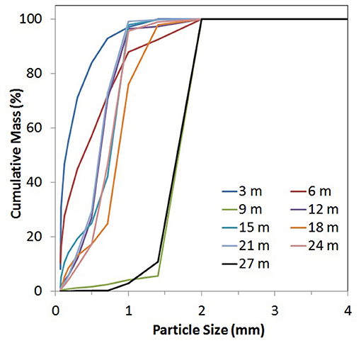
Figure 3. Particle size distribution of the NUC well at 3-m depth interval.
Figure 4A shows the FFEC profiles for the ARH well as a function of depth, and Figure 4B shows the modified profiles, which were obtained using Eq. 2 (by subtracting the observed salinity profiles from the initial salinity value of 0.775 g/L). These figures show that the logging profile peaks between 14.5- and 16-m depths were increasing consistently with pumping time then normalized to the salinity of ambient groundwater, which is consistent with the conceptual model of the FFEC technique. The surface water level did not drop during the field experiment, and also, the salinity of their corresponding feed-points did not vary with time, which is further being analyzed in the modeling section. The later profiles clearly showed the influence of incoming native fluid with an increase in pumping time; the peaks were decreasing throughout the observation period while pumping. The relationship between the total mass of salt left in the wellbore as a function of time indicates that they were decreasing with pumping duration, as illustrated in Figure 5, which also supports the finding of Sharma et al. (2015).
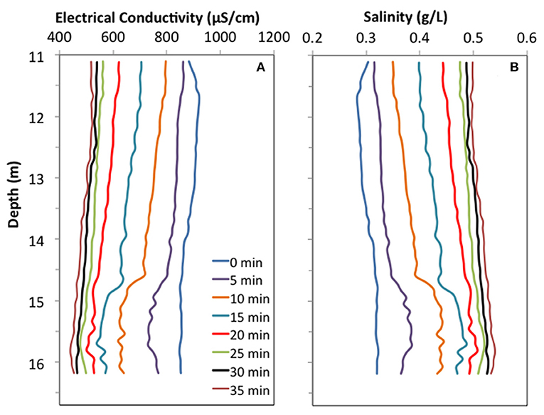
Figure 4. Logging data collected at ARH well: (A) original flowing fluid electrical conductivity (FFEC) profile (t = 0 min, profiles shows the background profile) and (B) modified salinity profile. The modified salinities were obtained from their corresponding electrical conductivity (ECs) by converting them using Eq. 3 and subtracting with a constant salinity value of 0.775 g/L.
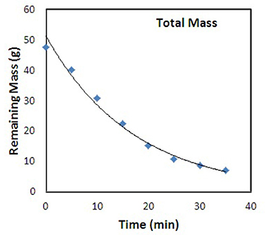
Figure 5. Total mass of salt remained in the wellbore as a function of time for the ARH well (the point shows the data, and the line indicates the trend).
The collected FFEC profiles at the NUC well, after replacement of original wellbore water with 1,600 μS/cm, are shown in Figure 6A, and the modified salinity profile after using Eq. 2 (by subtracting the observed salinity profiles from the initial salinity value of 1.23 g/L) is shown in Figure 6B. It was noted that the water table did not fluctuate during the logging period. Figure 7 indicates that a significantly high inflow zone exits at the bottom of the well (47-m depth), which would have influenced the wellbore salinity immediately after replacing the original fluid. Then there was also a high inflow zone present at the top of the study zone of the well (~16-m depth). Other prominent peaks can also be identified from the profile at 20- and 35-m depth before starting the modeling for detail characterization.
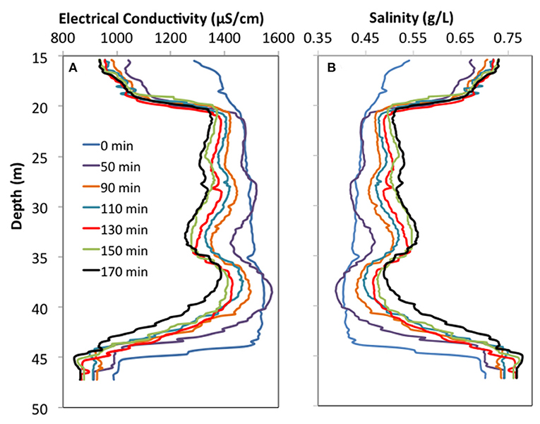
Figure 6. Logging data collected at the NUC well: (A) original FFEC profile (t = 0 min, profiles shows the background profile) and (B) modified salinity profile. The modified salinities were obtained from their corresponding ECs by converting them using Eq. 3 and subtracting with a constant salinity value of 1.23 g/L.
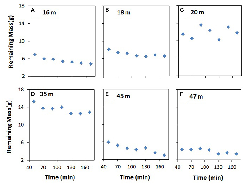
Figure 7. Remaining mass of salt in the wellbore as a function of time for the NUC well near the identified peaks at: (A) 16 m, (B) 18 m, (C) 20 m, (D) 35 m, (E) 45 m, and (F) 47 m.
Figure 7 shows the analysis of mass integral [M(t)] carried out for the major peaks at 47, 45, 35, 20, 18, and 16 m of the NUC well. Here M(t) denotes the mass of salt remaining in the wellbore (at the selected peaks with ±0.5 m around the peaks) with respect to the time under a constant pumping condition. For the constant feed point strength, ion concentration, and pumping condition, M(t) should decrease from time t = 0 min with the entrance of native fluid in the well. However, the M(t) vs. time plot shows that the salinity in the well at 20 and 35 m are decreasing more slowly than 16-, 18-, 45-, and 47-m depths, where the injected salt solution is mixing faster with the native water (Figure 7). Interestingly, for 16 and 18 m, this mixing tends to slow down after 70 min, whereas for 45 and 47 m, the mixing with the native water continues until 170 min. This may be due to the presence of large fractures at the bottom of this newly constructed borewell until the bedrock, which might have saturated the wellbore water very fast through the bottom of the well. Figure 8 indicates the total salt mass present in the wellbore as a function of time. It hints a linear decrease in total salt mass throughout the pumping period, which is slightly different from the sum of the salt mass near the selected individual peaks shown in Figure 7. This may be due to the overall salinity distribution along the borewell, which followed a linear decrease compared with the measured salinity just near the highly conductive zones or fractures. It can also be noted that the total salt mass in the well (in Figure 8) should be higher than the sum of the remaining salt mass (in Figure 7), in which only 1-m range near each peak was considered for these calculations.
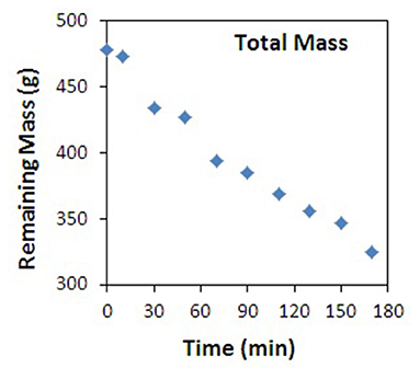
Figure 8. Total mass of salt remained in the wellbore as a function of time for the NUC well.
The background profile (profile at t = 0 min) was used as initial or baseline condition, and profiles for t = 5, 10, 15, and 20 min were selected for simulation using the BORE II model. The best fit for the profile at 15 min overlapped well with the other profiles for this site, as depicted in Figure 9. The corresponding inflow strength and concentration are listed in Table 1. For the simulation of ARH concentration profiles, 1 × 10⁻⁵ m2/s was used as a diffusion coefficient, and a constant salinity of 0.55 g/L was used as wellbore native water concentration. To get the ambient concentration of the wellbore water, the constant salinity (0.55 g/L) value was subtracted from the initial salinity (0.775 g/L), and this reverse transformation provides the actual wellbore water salinity as 0.225 g/L.
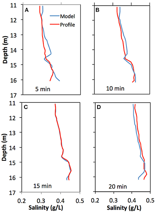
Figure 9. Modeling of selected profiles for the ARH well at: (A) 5 min, (B) 10 min, (C) 15 min, and (D) 20 min.
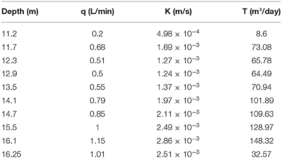
Table 1. Flow strength and concentration obtained from BORE II modeling and estimated transmissivities for the Ajatshatru Residential Hall (ARH) well.
In Table 1, the estimation of their corresponding hydraulic conductivities was also shown using Darcy's law by approximating the hydraulic gradient from a neighboring well and flow rate were estimated from respective model values. The hydraulic gradient was estimated from a nearby well 28.4 m from the logged well with a water level difference of 0.2 m, and the area of porous media was considered at 0.957 m2. The hydraulic conductivity values were high around this well due to relatively high porous media conductivity near 16 m of depth. The hydraulic conductivity values were almost similar throughout the well, and it had a slightly higher flow rate at the bottom of the well. The hydraulic conductivities were observed in the range of 5 × 10⁻⁴ to 3 × 10⁻³ m/s (Table 1). Although these estimated hydraulic conductivities were based on the hydraulic gradient in one direction using two neighboring wells only, the estimates can be indicative to understand the approximate hydrogeology near the selected site for ASR feasibilities.
The background profile (profile at t = 0 min) obtained at the NUC well was used as an initial condition or baseline for the model. It was difficult to model the initial profiles due to sudden changes in salinity from the bottom of the well through large fractures. Therefore, for these tests, profiles at time equal to 110, 130, 150, and 170 min were used for the simulation. In this case, 6 × 10⁻⁵ m2/s was used as a diffusion coefficient, and a constant native wellbore concentration of 0.856 g/L was assumed for the modeling of NUC concentration profiles. Similar to the previous case, the input concentration (0.856 g/L) value was subtracted from the total (1.23 g/L) value for modifying the profile. This reverse transformation of concentration value provides the actual salinity value of the wellbore water as 0.374 g/L.
The best-fit from the model for these profiles from the NUC site is shown in Figure 10. They were enough to indicate the important features of the permeable zones intersecting the wellbore for depth up to 47 m. Since the wellbore is situated in a non-fractured aquifer, the water entered from all over the studied section would have happened. The lowermost and the topmost part of the well had higher inflow strengths as expected from the measured profiles. The high inflow strengths were obtained at 16, 18, 20, 36, 44, and 46 m as 0.138, 0.21, 0.476, 0.073, 0.054, and 2.683 L/min, respectively (as shown in Table 2). The lowest zone had relatively high inflow strength, which may be due to the high flow rate from the bottom of the well. As mentioned earlier, the well was drilled until 60 m, but they were not accessible due to mud or sand filled through the screen until 47-m depth at the time of this field study. It may also be possible that water might be entering from the fractures near the bedrock at the bottom of the well.
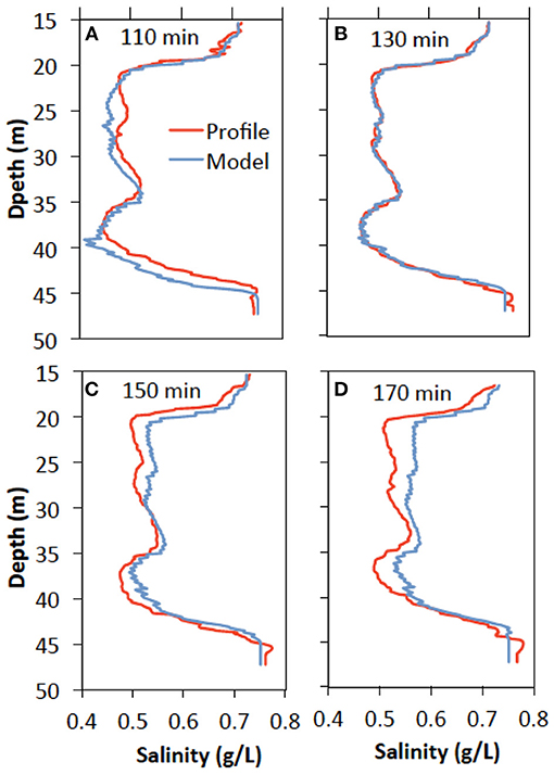
Figure 10. Modeling of selected profiles for the NUC well at: (A) 110 min, (B) 130 min, (C) 150 min, and (D) 170 min.
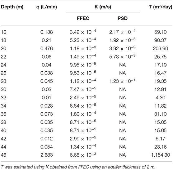
Table 2. Flow strength (q) and concentration (C) obtained from BORE II modeling and estimated transmissivities, K from flowing fluid electrical conductivity (FFEC) modeling, and approximated using Eq. 1 and particle size distribution (PSD) for the Nalanda University Campus (NUC) well.
Hydraulic conductivity (K) of each flow zone was calculated using Darcy's law, for which a nearby well from a distance of 646.453 m and water level difference of 4.52 were used to estimate the hydraulic gradient and area of 0.957 m2 was considered. High hydraulic conductivities were observed at 46 m as 6.68 × 10⁻³ m/s and at 20 m as 1.18 × 10⁻³ m/s; however, the lowest hydraulic conductivity was observed at 32 m as 2.49 × 10⁻⁵ m/s. All other K values with volumetric flow rates at different depth ranges are shown in Table 2, but are not congruent with the hydraulic conductivity estimated through particle size distribution. These measurements show that these layers comprised medium sand to coarse sand; however, the particle size distribution of the NUC well categorized the soil to be very fine-to-medium sand. For these minor deviations, it can be postulated that PSD was just a point value for the borehole samples and does not need to correspond to flow in the sand layers. This paper also warns against the use of PSD for the prediction of groundwater flow patterns directly. These FFEC logging results showed different layers of sand, which was also falling in a similar range with the previous lithological studies (Chakroborty and Chattopadhyay, 2001; Saha et al., 2010). The hydrogeological study conducted in the same district estimated an average hydraulic conductivity through time drawdown data interpretation and found an average K ranged from 1.01 × 10⁻⁴ to 9.68 × 10⁻⁴ m/s (Saha et al., 2010). The average K values from this study for the NUC site was found at 2.13 × 10⁻⁴ m/s for a depth range of 15 to 45 m, which was close to the K value of 1.99 × 10⁻⁴ m/s for another nearby test location at Islampur with a similar geographical feature and near the foothills of Rajgir as reported by Saha et al. (2010).
Transmissivity was estimated by the multiplication of hydraulic conductivity with the corresponding aquifer thickness. At ARH, the transmissivity of the main conductive aquifer (6-m thickness) was approximately 804 m2/day, and at NUC, the aquifer thickness was 6 m from 16 to 22 m bgl with a transmissivity of 353 m2/day and 2 m from 45 to 47 m bgl with a transmissivity of 1,154 m2/day, which can potentially be utilized as a storage zone for ASR application. These high conductive zones can be a target zone for storing excess water available during the rainy season. However, these high conductive zones are very small (less than 8 m) for the medium- to large-scale ASR (injection rate >100 m3/day), which may not be suitable for a large-scale injection in the agricultural fields (excess water from low-lying areas in that area). Like in the ASR wells of the United States, where the injection rates were reported from 757 to 8,705 m3/day with an approximate recovery rate of 3,785 m3/day (Bloetscher, 2015; Bloetscher et al., 2020). The previous ASR guidelines suggest that the large-scale ASR should have high transmissivities with relatively large aquifer thickness (more than 8 m) so that a large amount of water can be injected efficiently and economically (Stuyfzand et al., 2002; Pavelic et al., 2006; Izbicki et al., 2010; Page et al., 2014; Sultana et al., 2015). Apart from transmissivities and aquifer thickness constraints, it was found that maximum discharge of the well was less than 100 L/min at both the sites, and similar scenarios had been observed adjacent to the study area in shallow aquifers. This pumping rate may not be economically suitable for agriculture use, but these shallow aquifers are extensively being used for household usage in this region. These shallow aquifers generally get dry during the summer season, which can be replenished by injecting the rooftop rainwater during the monsoon, as recommended by the Central Ground Water Board. (2003). As the FFEC and modeling results showed that the aquifers have high transmissivities with small thickness, it can be adequate for small-scale ASR, i.e., an injection rate lower than 20 m3/day. Rooftop water is generally considered of good quality if the roof is cleaned regularly, which can further be improved with a basic activated charcoal filter system for a small-scale ASR. Cost of drilling and filtration systems are quite low than a sophisticated large-scale filtration system, which generally requires deeper borewells. This study was limited to shallow borewells and for agricultural water usage so the water banking for a deeper aquifer needs to be explored for the feasibility of large-scale ASR for this region of South Bihar. A further investigation is required to develop a low-cost ASR for a deeper aquifer so that this managed aquifer recharge method gets adopted on a large scale to conserve the rainwater and improve the economic condition of this region through agricultural income.
This study was conducted to analyze the hydrogeological feasibility of ASR in the shallow aquifers for irrigation and household usage at Rajgir, Bihar, India. With FFEC and BORE II modeling, transmissivities and thickness of hydraulically conductive aquifers at the studied sites were estimated for possible aquifer storage. At both selected sites, the high conductive zones of small thicknesses were found in the upper aquifers, which may not be desirable for investing in ASR for large waterlogged agricultural fields of South Bihar. Discharge rates at both sites were low, which may also be challenging for the recovery of stored water. Hence, these aquifers may not be fruitful for the medium- to large-scale ASR installations in the shallow aquifers. However, a small-scale ASR can be effectively developed in these shallow aquifers for storing the rooftop runoff water during the rainy season, which can augment the groundwater to these aquifers. This small-scale ASR can be very economical and can be adopted mainly at household, commercial, or official building level for recharging and storing the excess water in aquifers for dealing with the issues of water scarcity and declining groundwater level of this region. For medium- to large-scale ASR, deeper aquifers need to be investigated further for the ASR feasibility.
The original contributions presented in the study are included in the article/Supplementary Material, further inquiries can be directed to the corresponding author/s.
AV worked on data collection, conceptualisation, and writing the paper. PS designed and conceptualised the work and reviewed and supervised the work. All authors contributed to the article and approved the submitted version.
A grant (WAC/2018/211) from the Australian Centre for International Agricultural Research for supporting this research is greatly acknowledged.
The authors declare that the research was conducted in the absence of any commercial or financial relationships that could be construed as a potential conflict of interest.
All claims expressed in this article are solely those of the authors and do not necessarily represent those of their affiliated organizations, or those of the publisher, the editors and the reviewers. Any product that may be evaluated in this article, or claim that may be made by its manufacturer, is not guaranteed or endorsed by the publisher.
We would like to acknowledge the useful advice from Dr. Chin-Fu Tsang in designing the setup and improving the manuscript.
The Supplementary Material for this article can be found online at: https://www.frontiersin.org/articles/10.3389/frwa.2021.802095/full#supplementary-material
Aadhar, S., and Mishra, V. (2020). On the projected decline in droughts over South Asia in CMIP6 multimodel ensemble. J. Geophys. Res. 125, e2020JD033587. doi: 10.1029/2020JD033587
Alqahtani, A., Sale, T., Ronayne, M. J., and Hemenway, C. (2021). Demonstration of sustainable development of groundwater through aquifer storage and recovery (ASR). Water Resour. Manage. 35, 429–445. doi: 10.1007/s11269-020-02721-2
Bandyopadhyay, S., Sharma, A., Sahoo, S., Dhavala, K. K., and Sharma, P. (2021). Potential for Aquifer Storage and Recovery (ASR) in South Bihar, India. Sustainability. 13, 3502. doi: 10.3390/su13063502
Bloetscher, F. (2015). M63 Aquifer Storage and Recovery. American Water Works Association. Vol. 63. doi: 10.12999/AWWA.M63ed1
Bloetscher, F., Sham, C. H., and Ratick, S. J. (2020). Aquifer Storage and Recovery: Can an Updated Inventory Predict Future System Success?. J. Am. Water Works Assoc. 112, 48–55. doi: 10.1002/awwa.1594
Bouwer, H. (2002). Artificial recharge of groundwater: hydrogeology and engineering. Hydrogeol. J. 10, 121–142. doi: 10.1007/s10040-001-0182-4
Brown, C. J., Weiss, R., Verrastro, R., and Schubert, S. (2005). Development of an aquifer, storage and recovery (ASR) site selection suitability index in support of the comprehensive everglades restoration project. J. Environ. Hydrol. 13, 1–13.
Central Ground Water Board. (2003). Rain water harvesting techniques to augment ground water. Available online at: http://cgwb.gov.in/documents/RWH_GUIDE.pdf (accessed September 20, 2021).
Central Ground Water Board. (2013). Groundwater information booklet Nalanda district, Bihar State. Available online at: http://cgwb.gov.in/District_Profile/Bihar/Nalanda.pdf (accessed September 20, 2021).
Chakroborty, C., and Chattopadhyay, G. S. (2001). Quaternary geology of south Ganga plain in Bihar. Indian Miner. 55, 133–142.
Collins, S. L., and Bianchi, M. (2020). DISOLV: a Python package for the interpretation of borehole dilution tests. Groundwater 58, 805–812. doi: 10.1111/gwat.12992
Cotterman, K. A., Kendall, A. D., Basso, B., and Hyndman, D. W. (2018). Groundwater depletion and climate change: future prospects of crop production in the Central High Plains Aquifer. Clim. Change. 146, 187–200. doi: 10.1007/s10584-017-1947-7
Dillon, P., Stuyfzand, P., Grischek, T., Lluria, M., Pyne, R. D. G., Jain, R. C., et al. (2019). Sixty years of global progress in managed aquifer recharge. Hydrogeol. J. 27, 1–30. doi: 10.1007/s10040-018-1841-z
Doughty, C., Takeuchi, S., Amano, K., Shimo, M., and Tsang, C. F. (2005). Application of multirate flowing fluid electric conductivity logging method to well DH-2, Tono Site, Japan. Water Resour. Res. 41, 1–16. doi: 10.1029/2004WR003708
Doughty, C., and Tsang, C.-F. (2000). BORE II?A code to compute dynamic wellbore electrical-conductivity logs with multiple inflow/outflow points including the effects of horizontal flow across the well. Rep. LBL-46833, Berkeley, CA: Lawrence Berkeley Natl. Lab., 2000.
Doughty, C., and Tsang, C. F. (2005). Signatures in flowing fluid electric conductivity logs. J. Hydrol. 310, 157–180. doi: 10.1016/j.jhydrol.2004.12.003
Doughty, C., Tsang, C. F., Hatanaka, K., Yabuuchi, S., and Kurikami, H. (2008). Application of direct-fitting, mass integral, and multirate methods to analysis of flowing fluid electric conductivity logs from Horonobe, Japan. Water Resour. Res. 44, 1–19. doi: 10.1029/2007WR006441
Doughty, C., Tsang, C. F., Rosberg, J. E., Juhlin, C., Dobson, P. F., and Birkholzer, J. T. (2017). Flowing fluid electrical conductivity logging of a deep borehole during and following drilling: estimation of transmissivity, water salinity and hydraulic head of conductive zones. Hydrogeol. J. 25, 501–517. doi: 10.1007/s10040-016-1497-5
Doughty, C., Tsang, C. F., Yabuuchi, S., and Kunimaru, T. (2013). Flowing fluid electric conductivity logging for a deep artesian well in fractured rock with regional flow. J. Hydrol. 482, 1–13. doi: 10.1016/j.jhydrol.2012.04.061
Elshall, A. S., Arik, A. D., El-Kadi, A. I., Pierce, S., Ye, M., Burnett, K. M., et al. (2020). Groundwater sustainability: a review of the interactions between science and policy. Environ. Res. Lett. 15, 093004. doi: 10.1088/1748-9326/ab8e8c
Evans, D. G. (1995). Inverting fluid conductivity logs for fracture inflow parameters. Water Resour. Res. 31, 2905–2915. doi: 10.1029/95WR02482
Gee, G. W., and Or, D. (2002). 2.4 Particle-size analysis. Method. Soil Analy. 5, 255–293. doi: 10.2136/sssabookser5.4.c12
Guhathakurta, P., Sudeepkumar, B. L., Menon,P Prasad, A. K., Sangwan, N., and Advani, S. C. (2020). Observed Rainfall Variability and Changes over Bihar State. Climate Research and Services (Met Monograph No.: ESSO/IMD/HS/Rainfall Variability/04(2020)/28). Indian Meteorological Department. Available online at: http://imdpune.gov.in/hydrology/rainfall%20variability%20page/bihar_final.pdf.
Hale, F. V., and Tsang, C. F. (1988). A Code to Compute Borehole Fluid Conductivity Profiles With Multiple Feed Points (No. LBL-24928). Lawrence Berkeley Lab., CA (USA). doi: 10.2172/5100624
Izbicki, J. A., Petersen, C. E., Glotzbach, K. J., Metzger, L. F., Christensen, A. H., Smith, G. A., et al. (2010). Aquifer Storage Recovery (ASR) of chlorinated municipal drinking water in a confined aquifer. Appl. Geochem. 25, 1133–1152. doi: 10.1016/j.apgeochem.2010.04.017
Karasaki, K., Freifeld, B., Cohen, A., Grossenbacher, K., Cook, P., and Vasco, D. (2000). A multidisciplinary fractured rock characterization study at Raymond field site, Raymond, CA. J. Hydrol. 236, 17–34. doi: 10.1016/S0022-1694(00)00272-9
LaHaye, O., Habib, E. H., Vahdat-Aboueshagh, H., Tsai, F. T. C., and Borrok, D. (2021). Assessment of Aquifer Storage and Recovery Feasibility Using Numerical Modeling and Geospatial Analysis: Application in Louisiana. JAWRA Journal of the American Water Resources Association. doi: 10.1111/1752-1688.12923
Maliva, R. G., Clayton, E. A., and Missimer, T. M. (2009). Application of advanced borehole geophysical logging to managed aquifer recharge investigations. Hydrogeol. J. 17, 1547–1556. doi: 10.1007/s10040-009-0437-z
Maliva, R. G., and Missimer, T. M. (2010). “Aquifer storage and recovery and managed aquifer recharge using wells: Planning, hydrogeology, design, and operation.” Methods in water resources evaluation, Schlumberger Water Services, TX.
Page, D., Vanderzalm, J., Miotliński, K., Barry, K., Dillon, P., Lawrie, K., et al. (2014). Determining treatment requirements for turbid river water to avoid clogging of aquifer storage and recovery wells in siliceous alluvium. Water Res. 66, 99–110. doi: 10.1016/j.watres.2014.08.018
Page, D. W., Peeters, L., Vanderzalm, J., Barry, K., and Gonzalez, D. (2017). Effect of aquifer storage and recovery (ASR) on recovered stormwater quality variability. Water Res. 117, 1–8. doi: 10.1016/j.watres.2017.03.049
Paillet, F. L., and Pedler, W. H. (1996). Integrated borehole logging methods for wellhead protection applications. Eng. Geol. 42, 155–165. doi: 10.1016/0013-7952(95)00077-1
Pavelic, P., Dillon, P. J., and Simmons, C. T. (2006). Multiscale characterization of a heterogeneous aquifer using an ASR operation. Groundwater 44, 155–164. doi: 10.1111/j.1745-6584.2005.00135.x
Petkewich, M. D., Parkhurst, D. L., Conlon, K. J., Campbell, B. G., and Mirecki, J. E. (2004). Hydrologic and Geochemical Evaluation of Aquifer Storage Recovery in the Santee Limestone/Black Mingo Aquifer, Charleston, South Carolina, 1998–2002. US Geological Survey: Reston, VA, USA. doi: 10.3133/sir20045046
Pyne, R. D. G. (2005). Aquifer storage recovery: a guide to groundwater recharge through wells. ASR systems.
Rodell, M., Velicogna, I., and Famiglietti, J. S. (2009). Satellite-based estimates of groundwater depletion in India. Nature 460, 999–1002. doi: 10.1038/nature08238
Roxy, M. K., Ghosh, S., Pathak, A., Athulya, R., Mujumdar, M., Murtugudde, R., et al. (2017). A threefold rise in widespread extreme rain events over central India. Nat. Commun. 8, 1–11. doi: 10.1038/s41467-017-00744-9
Saha, D., Dhar, Y. R., and Vittala, S. S. (2010). Delineation of groundwater development potential zones in parts of marginal Ganga Alluvial Plain in South Bihar, Eastern India. Environ. Monitor. Assess. 165, 179–191. doi: 10.1007/s10661-009-0937-2
Sharma, P., Tsang, C. F., Doughty, C., Niemi, A., and Bensabat, J. (2015). Feasibility of Long-Term Passive Monitoring of Deep Hydrogeology with Flowing Fluid Electric Conductivity Logging Method. Fluid Dynamics in Complex Fractured-Porous Systems. p. 53–62. doi: 10.1002/9781118877517.ch4
Sharma, P., Tsang, C. F., Kukkonen, I. T., and Niemi, A. (2016). Analysis of 6-year fluid electric conductivity logs to evaluate the hydraulic structure of the deep drill hole at Outokumpu, Finland. Int. J. Earth Sci. 105, 1549–1562. doi: 10.1007/s00531-015-1268-x
Stuyfzand, P. J., Vogelaar, A. J., and Wakker, J. (2002). September. Hydrogeochemistry of prolonged deep well injection subsequent aquifer storage in pyritiferous sands; DIZON pilot, Netherlands. In: Dillon, P.J. (Ed.), Management of Aquifer Recharge for Sustainability. Proc. 4th Int. Symp. Artificial Recharge of Groundwater, Adelaide, South Australia. p. 22–26.
Suhag, R. (2016). Overview of ground water in India. Delhi: PRS Legislative Research Standing Committee on Water Resources.
Sultana, S., Ahmed, K. M., Mahtab-Ul-Alam, S. M., Hasan, M., Tuinhof, A., Ghosh, S. K., et al. (2015). Low-cost aquifer storage and recovery: implications for improving drinking water access for rural communities in coastal Bangladesh. J. Hydrol. Eng. 20, B5014007. doi: 10.1061/(ASCE)HE.1943-5584.0001100
Tsang, C. F., Hufschmied, P., and Hale, F. V. (1990). Determination of fracture inflow parameters with a borehole fluid conductivity logging method. Water Resour. Res. 26, 561–578. doi: 10.1029/WR026i004p00561
Vanderzalm, J., Page, D., Regel, R., Ingleton, G., Nwayo, C., and Gonzalez, D. (2020). Nutrient transformation and removal from treated wastewater recycled via Aquifer Storage and Recovery (ASR) in a carbonate aquifer. Water, Air, and Soil Pollut. 231, 1–12. doi: 10.1007/s11270-020-4429-x
Wada, Y., Wisser, D., and Bierkens, M. F. (2014). Global modeling of withdrawal, allocation and consumptive use of surface water and groundwater resources. Earth Syst. Dyn. 5, 15–40. doi: 10.5194/esd-5-15-2014
Yaduvanshi, A., Srivastava, P. K., and Pandey, A. C. (2015). Integrating TRMM and MODIS satellite with socio-economic vulnerability for monitoring drought risk over a tropical region of India. Phys. Chem. Earth A/B/C. 83, 14–27. doi: 10.1016/j.pce.2015.01.006
Zuurbier, K. G., Kooiman, J. W., Groen, M. M., Maas, B., and Stuyfzand, P. J. (2015). Enabling successful aquifer storage and recovery of freshwater using horizontal directional drilled wells in coastal aquifers. J. Hydrol. Eng. 20, B4014003. doi: 10.1061/(ASCE)HE.1943-5584.0000990
Keywords: groundwater recharge, aquifer storage and recovery, transmissivity, aquifer thickness, well logging
Citation: Verma A and Sharma P (2022) Aquifer Storage and Recovery Feasibility Study With Flowing Fluid Electrical Conductivity Logging in Shallow Aquifers of South Bihar, India. Front. Water 3:802095. doi: 10.3389/frwa.2021.802095
Received: 26 October 2021; Accepted: 25 November 2021;
Published: 07 January 2022.
Edited by:
Nitin Joshi, Indian Institute of Technology Jammu, IndiaReviewed by:
Mustafa El-Rawy, Minia University, EgyptCopyright © 2022 Verma and Sharma. This is an open-access article distributed under the terms of the Creative Commons Attribution License (CC BY). The use, distribution or reproduction in other forums is permitted, provided the original author(s) and the copyright owner(s) are credited and that the original publication in this journal is cited, in accordance with accepted academic practice. No use, distribution or reproduction is permitted which does not comply with these terms.
*Correspondence: Prabhakar Sharma, cHNoYXJtYUBuYWxhbmRhdW5pdi5lZHUuaW4=
Disclaimer: All claims expressed in this article are solely those of the authors and do not necessarily represent those of their affiliated organizations, or those of the publisher, the editors and the reviewers. Any product that may be evaluated in this article or claim that may be made by its manufacturer is not guaranteed or endorsed by the publisher.
Research integrity at Frontiers
Learn more about the work of our research integrity team to safeguard the quality of each article we publish.