A Multi-Year Assessment of Phytoplankton Fluorescence in a Large Temperate River Reveals the Importance of Scale-Dependent Temporal Patterns Associated With Temperature and Other Physicochemical Variables

An integrated temporal study of a long-term ecological research and monitoring database of the St. Lawrence River was carried out. A long and mostly uninterrupted high temporal resolution record of fluorometric data from 2014 to 2018 was used to examine phytoplankton fluorometric variables at several scales and to identify temporal patterns and their main environmental drivers. Sets of temporal eigenvectors were used as modulating variables in a multiscale codependence analysis to relate the fluorometric variables and various environmental variables at different temporal scales. Fluorometric patterns of phytoplankton biomass in the St. Lawrence River are characterized by large, yearly-scale patterns driven by seasonal changes in water temperature, and to a lesser extent water discharge, over which finer-scale temporal patterns related to colored dissolved organic matter and weather variables can be discerned at shorter time scales. The results suggest that such an approach to characterize phytoplankton biomass in large rivers may be useful for processing large data sets from remote sensing efforts for detecting subtle large-scale changes in water quality due to land use practices and climate change.

Introduction

The Upper St. Lawrence River (CA, US) represents an ecological, economic, cultural, and socially important ecosystem (Lean, 2000; Twiss, 2007; Marty et al., 2010). Increased knowledge of the patterns of water quality and its main drivers is valuable for the assessment and management of priority resources such as fish populations. To this end, detection of tributary and point-source inputs that result in nutrient enrichment and fecal bacterial contamination (Bramburger et al., 2015), mercury mobilization from changing water levels (Brahmstedt et al., 2019), and harmful cyanobacterial blooms with related taste and odor issues (Watson et al., 2008), are necessary. However, the possible existence of patterns at several temporal scales makes the inference of results strongly dependent on the respective scale of the study. Scale becomes an important factor not only for ecological studies, but also for management purposes, as management projects can fail if they use information based on small-scale patterns to modify larger-scale patterns when there is a disconnect between the two. For example, if the variables affecting daily variation are different than those affecting yearly variation, then considering them to develop programs at the yearly scale will possibly lead to failure.

Long-term ecosystem research and monitoring (LTERM) programs are essential to assess and study various temporal scales simultaneously. Long-term datasets represent the best possible approach to studying multiple scales in a single analysis. In addition, an important approach to LTERM is the application of techniques that can handle such data so that processes that impact environmental change can be detected and understood with the aim of informing ecosystem-based management actions (Parr et al., 2003). Within the Great Lakes-St. Lawrence River system there are a limited number of sensor arrays capable of supporting LTERM with very few deployed in the large rivers that provide lake-to-lake drainage throughout this system. There is also the limitation that buoy-based sensors are restricted to ice-free periods, typically May to December (Twiss and Stryszowska, 2016). Here we use a novel observation platform by placing water quality sensors inside of a hydroelectric power dam, which affords year round observations at high degrees of temporal resolution (minutes) over the span of years. In situ phytoplankton fluorescence techniques have been widely used in aquatic systems to estimate phytoplankton biomass levels and dynamics (reviewed by Bae and Park, 2014); however, studies are typically limited to episodic surveys over short time frames.

This study represents an integrated temporal study of a LTERM database of phytoplankton fluorescence in the St. Lawrence River. Using a mostly uninterrupted dataset that covers a moderate temporal extent (~5 years between 2014 and 2019 including several record high water years), phytoplankton fluorometric variables at several temporal scales were examined to identify temporal patterns and their main drivers to better understand the patterns of phytoplankton variables in the region of the Upper St. Lawrence River. Sets of temporal eigenvectors were used as modulating variables in multiscale codependence analysis (MCA) to relate the fluorometric variables and various environmental variables at different scales. The temporal eigenvectors related to the environmental variables from the MCA were combined into tables that represent biologically interesting environmental drivers and their influence on fluorometric variables assessed using variation partitioning.

Methods

Study Site and Data Acquisition

The Moses-Saunders hydropower dam is located on the St. Lawrence River, between the state of New York (USA) and the province of Ontario (Canada). A multi-sensor array installed in Unit 32 power turbine of the Moses-Saunders hydroelectric dam, along the New York shoreline of the St. Lawrence River (45°0.253′N, 74°47.945′W, Figure 1) gathered water quality data. The array consists of a Turner Designs (Sunnyvale, CA) C6 multi-sensor platform equipped with Cyclops-7 sondes. The array measures numerous water quality variables at 1–2 min intervals. Of interest in this analysis are water temperature, in vivo chlorophyll a, in vivo phycocyanin and colored dissolved organic matter (CDOM) fluorescence. Water from the penstock was drawn via a 30 cm diameter pipe used to cool the stator of the turbine-driven electric generator. This water is effectively mixed surface and bottom (~20 m depth) river water but is restricted to water that flows along the southern shoreline of the river owing to the location of the Unit 32 turbine, which is nearest to that shore. The C6 was housed in a watertight flow-through cell and is connected to the cooling water pipe via a stainless-steel pipe (1 cm diameter) with a pressure reduction gate valve. The array is equipped with an anti-fouling brush, which performs three revolutions prior to recording water quality observations to prevent any fouling by debris or organisms on the optical sensor surfaces. The entire system was visited at 2–3-week intervals to download data, clean instruments, and recalibrate.

FIGURE 1

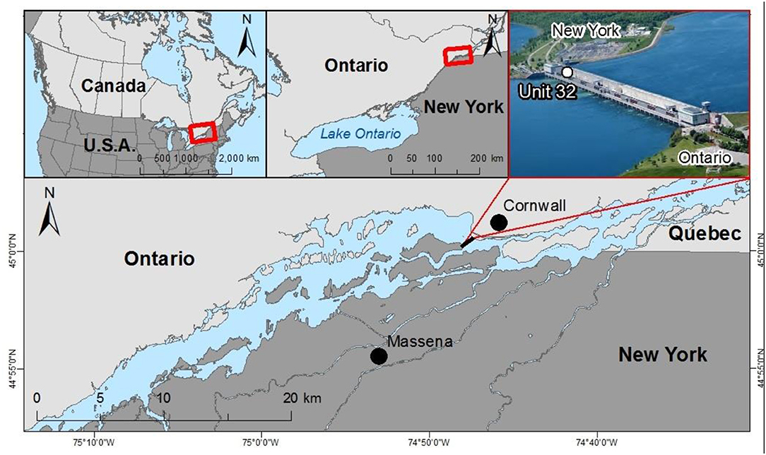
Figure 1. Geographical location of the Unit 32 power turbine of the Moses-Saunders hydroelectric dam on the Upper St. Lawrence River.

In addition to the data from the C6, two additional independent datasets were used. The first of these is a dataset of local atmospheric variables from the National Oceanic and Atmospheric Administration website (https://www.ncdc.noaa.gov) for a weather station near the study region (station number WBAN:94725; located 9 km distant at the Massena, NY airport). Variables that were measured on an hourly basis were retained for the analysis. These consist of air temperature (dry bulb temperature), wind speed and direction, visibility, precipitation, weather type and sky clarity (in oktas). Details regarding the NOAA variables and their measurement are available at https://www.ncdc.noaa.gov/cdo-web/datasets. The second of these is a dataset of daily water discharge in the St. Lawrence River at this site were obtained from the United States Geological Survey website (https://www.usgs.gov) through its National Water Information System web interface (station number 04264331).

Data were cleaned to remove any data collected during periods of water flow restrictions due to instrument clogging (infrequent) or maintenance by the dam operators (intermittent). Data were averaged into 4-h blocks to avoid overly long computing times and memory roadblocks during analyses. We found that this was the best value that offered a tradeoff between computational efficiency and obtaining results within reasonable amounts of time. Additionally, a previous study (Mimouni et al., 2020) showed that few variables in the region reflect daily patterns and if they did then they were much less important in magnitude than those at larger scales.

Linear regression models and covariances are sensitive to outlier values, so it is often best to consider transformations of the variable (Legendre and Legendre, 2012). The measured variables were individually transformed to reduce skewness as much as possible. Hourly chlorophyll a and phycocyanin fluorescence, hourly wind speed and daily chlorophyll a and phycocyanin fluorescence were square root transformed. Hourly precipitation and daily precipitation were fourth root transformed. Hourly CDOM, daily CDOM and daily discharge were log transformed. Qualitative variables (weather type and sky clarity) were recoded as binary variables. Even though sky clarity is an ordinal variable, it was treated as a qualitative variable because of the presence of different cloud layers and because data were averaged into blocks, implying that several classes of sky cover could be observed in the same block. Due to the circular nature of wind direction, it was decomposed into eastern and northern components by computing the sine and cosine of the angular direction. The average of each wind direction was computed, and the resulting vectors were then normed to obtain components that lay on the unit circle.

Construction of Temporal Variables

Due to the long extent (~5 years) and high sampling frequency (4-h or daily blocks) of the datasets, several patterns at various scales can be present. Direct multiscale ordination (DMSO; Wagner, 2004) indicated that regression coefficients were not homogeneous across scales as the sums of the explained and residual variance of a multiple linear model between the fluorometric variables and the environmental variables often stepped out of the computed intervals (results not shown). Therefore, we opted to compute distance-based Moran Eigenvector Map (dbMEM, Dray et al., 2006) variables that express the structures at various scales and study these structures rather than the environmental variables directly. Fluorometric variables were regressed against a numeric variable expressing the time since the data started being recorded to test for linear trends in the data. These regressions were tested using 9,999 permutations of the reduced model residuals. Phytoplankton fluorescence variables showed significant linear trends over time. Consequently, residuals of the regression were considered as new response variables.

A variety of sets of dbMEM variables were computed and confronted against the fluorometric variables to find the best set of temporal predictors. As in Dray et al. (2006), we considered a simple binary connection scheme, a linear weighing function of distances $f_1\left(d_{xy}|d_{max}\right)=1-\frac{d_{xy}}{d_{max}}$, a concave-up weighing function of distances $f_2\left(d_{xy}|d_{max},\alpha \right)=1-{\left(\frac{d_{xy}}{d_{max}}\right)}^{\alpha }$ and a concave-down weighing function of distances $f_3\left(d_{xy}|\beta \right)=\frac{1}{d_{xy}^{\beta }}$. The value of d_max was set at 149.17 days for the hourly dataset and 149 days for the daily dataset, the value of the longest gap in each dataset. We introduce a family of distance weighing functions, which we refer to as “exponentially weighted distances.” The general form of the weighing functions is:

$\begin{array}{ll}{\text{A}}_{\left[i,j\right]}=f_{expo}\left({\text{D}}_{\left[i,j\right]}|g\left(.\right),\lambda \right)=e^{-\lambda g\left({\text{D}}_{\left[i,j\right]}\right)}& (1)\end{array}$

Where g(.) is a mathematical function and λ is a real coefficient. Using this formula, it turns out that all of the weighing functions of Dray et al. (2006) are special cases of the exponentially weighted distances family. For example, the concave-down function f₃ considers g(x) = log(x) and λ = β. We considered a square-root transformation of distances ($g\left(x\right)=\sqrt{x}$) and no transformation of distances [g(x) = x]. We also considered a weighing function that is similar to the concave-up function f₃, but more flexible. The function considers $g\left(x\right)=x^{k_1}$ and $\lambda =2^{-k_2}$. An additional advantage of this function over f₂ is that it never crosses the abscissa, therefore allowing for the weighing of any distance. The best-fitting dbMEM was selected based on maximizing the adjusted multiple determination coefficient, $R_{adj}^2$.

Codependence Analysis

The set of dbMEM variables that maximized $R_{adj}^2$ values were retained and used in multiscale codependence analysis (MCA, Guénard et al., 2010) to relate the different structures to environmental variables. All explanatory variables were also regressed on the linear trend expressing time and the residuals retained to avoid the appearance of spurious relationships before carrying out the MCA. Tests of significance for each codependence coefficient were carried out by parametric means.

The values of the codependence coefficients between the response and the explanatory variables were computed for each dbMEM variable. A positive codependence coefficient is indicative of a positive relationship between the two variables at the considered scale and conversely, a negative codependence coefficient is indicative of a negative relationship between the two variables. These values would allow us to separate among the positive and negative influences of the explanatory variables on phytoplankton fluorescence.

Variation Partitioning and Comparison of Fractions

The significant dbMEM variables in the MCA analysis were combined into different tables depending on the explanatory variable that showed the highest absolute codependence coefficient. Three tables were constructed for the hourly dataset and four tables for the daily dataset so that they represent biologically interesting environmental drivers. The first table consisted of air and water temperature (X1), the second table consisted of weather condition variables (X2) and the third table consisted of wind speed and direction, visibility as well as sky clarity (X3). The fourth table consisted of CDOM and, for the daily dataset only, water discharge (X4). Variation partitioning (Borcard et al., 1992; Borcard and Legendre, 1994) was used to compare the fractions of variation explained by each of the tables. Coefficients of multiple determination values were adjusted following Ezekiel's formula (Ezekiel, 1930; Peres-Neto et al., 2006). The significance of each individual fraction was tested using conditional regression and 9,999 permutations of the reduced model residuals.

Results

Environmental Conditions

The variables examined showed a considerable amount of variation (Table 1). A published database containing the sensor data collected from 2014 to 2019 is found at doi: 10.17632/8fpgm26drj.1. As expected from seasonal changes, water temperature varied between ~0.0°C in winter and up to 24.3°C in the summer. Wind direction was quite variable, even within 4-h blocks. At the largest scales, no clear structure was observed in the direction of the wind. Nonetheless, winds did not blow in an indiscriminate manner. Observation of the directional values of wind on the unit circle showed that northeasterly and southwesterly winds were the most common and southeasterly and northwesterly winds were the rarest. In terms of wind speed, values of up to 48 km·h⁻¹ were recorded.

TABLE 1

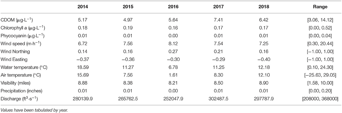
Table 1. Table of daily averages and ranges of the quantitative variables considered.

In vivo chlorophyll a fluorescence showed some amount of seasonal pattern, but it was not completely apparent. Even though seasonal highs of 0.4 μg·L⁻¹ and above in summer and lows of around 0.0 μg·L⁻¹ in winter could be observed, there were several more localized peaks, especially in late fall. In late fall of 2015, 2016, and 2017, a second peak of chlorophyll a was noted, after the summer peak had begun to subside. The peak in late 2015 was especially important, as it was on par with the summer peak of 2015. Phycocyanin also showed a seasonal pattern, but this was much clearer and stronger than chlorophyll a. Despite being more clearly periodic than chlorophyll a, phycocyanin also showed some localized peaks but the timing of these peaks were variable and did not always follow the late fall pattern found for chlorophyll a.

Construction of Temporal Variables

The best-fitting set of dbMEM variables differed depending on the considered fluorometric variable. For the hourly datasets, chlorophyll a was best explained by dbMEM variables constructed using parameters $g\left(x\right)=\sqrt{x}$ and λ = 5 and phycocyanin using values of $g\left(x\right)=\sqrt{x}$ and λ = 5. For the daily datasets, chlorophyll a was best explained by dbMEM variables constructed using parameters g(x) = log(x) and λ = 2 and phycocyanin using values of g(x) = log(x) and λ = 1.

Main Drivers of Fluorometric Variables

Tests of the significance of the MCA showed that, for the hourly datasets, 472 dbMEM variables were significant for chlorophyll a and 428 variables were significant for phycocyanin (in all cases, p ≤ 0.05). Likewise, for the daily datasets, 45 dbMEM variables were significant for chlorophyll a and 47 variables were significant for phycocyanin (in all cases, p ≤ 0.05). Codependence coefficients between the fluorometric variables and the environmental variables were quite variable, both in sign and magnitude.

For hourly datasets, adjusted fractions of variation explained by eigenvectors associated with each explanatory variable (Table 2) showed that dbMEM variables associated with water and air temperature explained most of the variation, as they explained close to three quarters of the variation in chlorophyll a and phycocyanin fluorescence. dbMEM variables associated with CDOM explained over 10% of the variation. Wind, weather and sky variables individually explained much smaller amounts of variation. However, the results somewhat differed for daily datasets (Table 3). For both chlorophyll a and phycocyanin, dbMEM variables associated with water temperature still showed the strongest total coefficient of multiple determination, with their value being slightly less than for the hourly data. Likewise, dbMEM variables associated with CDOM also explained over 10% of the variation. However, water discharge proved to be a variable that explained a sizeable amount of variation, especially for chlorophyll a, where it explained approximately a quarter of the variation.

TABLE 2

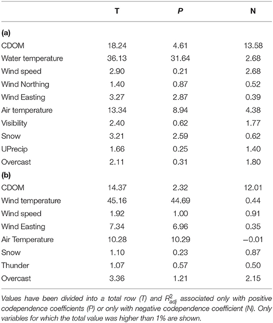
Table 2. Table of adjusted coefficients of multiple determination ($R_{adj}^2$) associated with the constructed dbMEM variables depending on the explanatory variable with which they showed the highest absolute codependence coefficient for hourly data of chlorophyll a (a) and phycocyanin (b).

TABLE 3

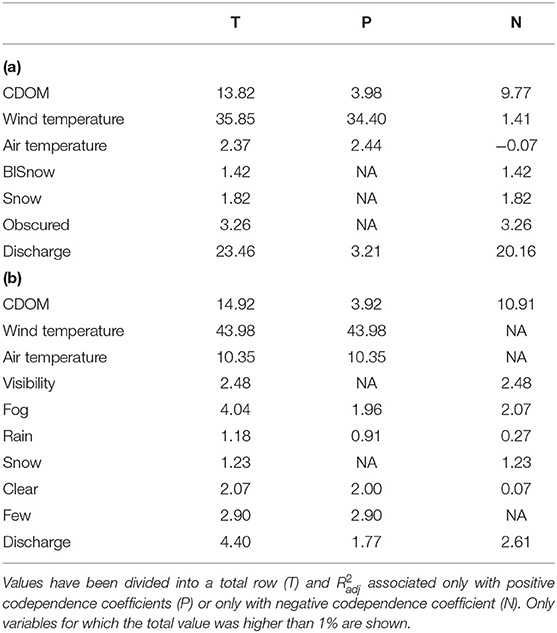
Table 3. Table of adjusted coefficients of multiple determination ($R_{adj}^2$) associated with the constructed dbMEM variables depending on the explanatory variable with which they showed the highest absolute codependence coefficient for daily data of chlorophyll a (a) and phycocyanin (b).

Computation and visualization of the fitted values of the fluorometric variables based on the different sets of dbMEM variables allowed visualization of the scales at which the patterns occurred for fluorometric variables. For both hourly datasets of phytoplankton fluorescence, dbMEM variables associated with water temperature were responsible for large-scale patterns, as the curve for the fitted values reflected seasonal patterns (Figure 2), especially for phycocyanin. In contrast, dbMEM variables associated with weather and sky variables were more localized and seemed to be associated with shorter-scale patterns. For daily of phytoplankton fluorescence, water temperature was still responsible for most of the large-scale variation, but only for phycocyanin (Figure 3). For chlorophyll a, it was still responsible for some large-scale pattern, but to a much smaller extent.

FIGURE 2

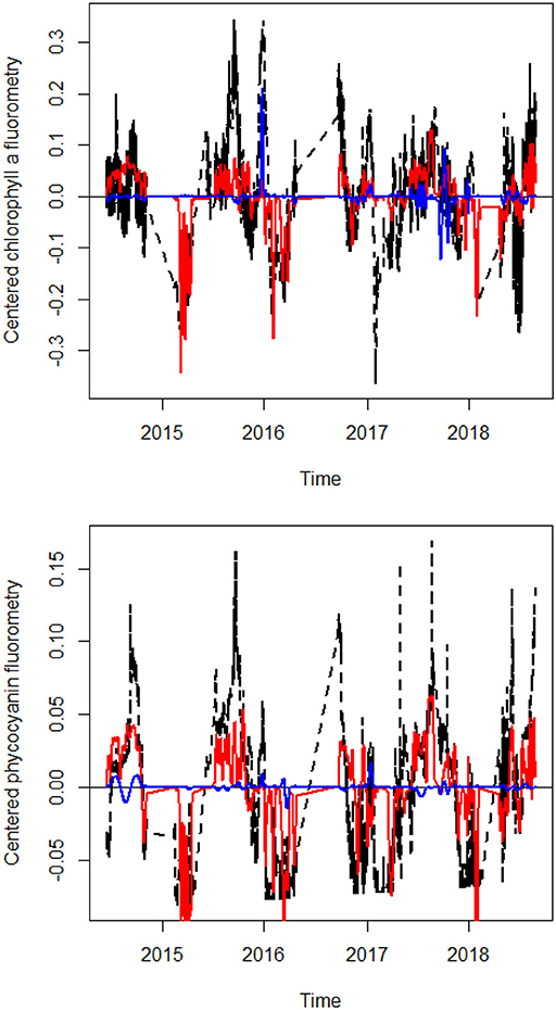
Figure 2. Line plots of hourly chlorophyll a and phycocyanin flurorometry, along with their fitted values according to the sets of dbMEM variables related to water temperature. Observed values are in black, fitted values relating to dbMEM variables related to water temperature are in red.

FIGURE 3

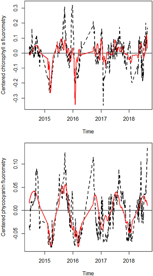
Figure 3. Line plots of daily chlorophyll a and phycocyanin flurorometry, along with their fitted values according to the sets of dbMEM variables related to water temperature. Observed values are in black, fitted values relating to dbMEM variables related to water temperature are in red.

It should be noted that the relationship between phytoplankton fluorescence and the explanatory variables could be either positive or negative. For water and air temperature, most of the variation was associated with positive codependence coefficients. This highlights a positive influence of temperature on phytoplankton fluorescence. However, for the daily datasets, some of the late fall peaks were shown to be negatively related to water discharge (see Figure 4). For other variables, adjusted fractions of variation associated with both negative and positive codependence coefficients were appreciable.

FIGURE 4

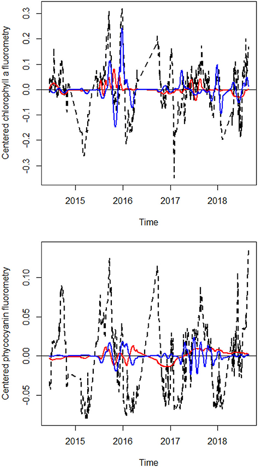
Figure 4. Line plots of daily chlorophyll a and phycocyanin flurorometry, along with their fitted values according to the sets of dbMEM variables related to water discharge. Observed values are in black, fitted values relating to dbMEM variables positively related to water discharge are in red and negatively related are in blue.

Variation Partitioning and Comparison of Fractions

Variation partitioning revealed that the most important part of the variation for both fluorometric variables in the hourly datasets was accounted for by dbMEM variables associated with temperature. This observation was more pronounced for phycocyanin than for chlorophyll a. dbMEM variables associated with temperature explained around half of the variation in chlorophyll a (54.1%) and phycocyanin (60.0%). For dbMEM variables associated with sky condition and CDOM, these variables accounted for less variation and respectively accounted for 18.1% and 20.3% of the variation for chlorophyll a and 19.0% and 16.0% of the variation for phycocyanin (see Figure 5). dbMEM variables associated with weather variables accounted for less variation and respectively accounted for 11.4% of the variation for chlorophyll a and 7.9% of the variation for phycocyanin (see Figure 5). Tests of partial RDA showed that all fractions were significant (p_value ≤ 0.05 in all cases).

FIGURE 5

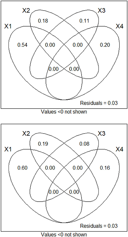
Figure 5. Variation partition diagram of hourly chlorophyll a and phycocyanin flurorometry between the three sets of dbMEM variables, as divided into ecologically interesting groups. See text for variable group explanations and denominations.

For daily chlorophyll a fluorescence, dbMEM variables associated with temperature explained the most variation (40.3%), followed by those associated with water discharge and CDOM (39.7%), then those associated with sky condition (5.9%) and finally those associated with weather variables (4.9%). For daily phycocyanin fluorescence, dbMEM variables associated with temperature explained the most variation (57.0%), followed by those associated with water discharge and CDOM (21.4%), then those associated with sky condition (12.1%) and finally those associated with weather variables (6.2%). The inclusion of dbMEM variables related to water discharge considerably changed results (see Figure 6). Tests of partial RDA showed that all fractions were significant (p_value ≤ 0.05 in all cases).

FIGURE 6

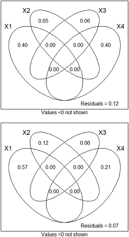
Figure 6. Variation partition diagram of daily chlorophyll a and phycocyanin flurorometry between the four sets of dbMEM variables, as divided into ecologically interesting groups. See text for variable group explanations and denominations.

Discussion

Both chlorophyll a and phycocyanin fluorescence showed discernable yearly patterns. These patterns are most likely related to yearly cycles in phytoplankton populations associated with annual variations in drivers of phytoplankton communities between the seasons in this temperate climate zone. This was especially true for phycocyanin, which showed a stronger yearly pattern than chlorophyll a. Chlorophyll a patterns differed considerably, as they were much more variable and showed several peaks late in the year after the summer peak. High resolution monitoring demonstrates that late fall chlorophyll a peaks are common in the Upper St. Lawrence River, as they occurred almost every year during the extent of the study. These events go against the established notion that phytoplankton productivity is only positively associated with increasing temperature and calls for a better understanding of the drivers of phytoplankton fluorescence in this large river system (annual average discharge in the Upper St. Lawrence River is ~8,000 m³·s⁻¹).

Nonetheless, it makes sense to consider temperature a prime driver of phytoplankton populations. Temperature can act positively both directly by influencing growth rate, as well as indirectly by influencing other variables in the water and positively correlates with light availability at this latitude in a temperate climate zone. In addition, the seasonal cyclical nature of temperature is well-suited to explain the yearly high values of fluorescence in summer and low values in winter. This hypothesis is supported by the results, as not only was a large fraction of the variation of phytoplankton fluorescence explained by temperature (either air or water) but was mostly comprised of structures that had a positive codependence coefficient.

However, temperature is not the only driver of phytoplankton fluorescence, and other driving variables should be considered. Light availability (day length) strongly relates to water temperature in this temperate climate and latitude (45°N). High light intensity can cause non-photochemical quenching of the phytoplankton photosynthetic apparatus, which is more sensitive to light regime than nutrient levels (Silsbe et al., 2015).

Using in vivo fluorescence (IVF) of chlorophyll-a is a rapid technique but requires appreciation of caveats. Chlorophylll-a IVF is affected by seasonal changes in phytoplankton populations, nutritional stress, and diel changes in ambient light levels (Loftus and Seliger, 1975; Kruskopf and Flynn, 2006). In this study there was diel variation of IVF of chlorophyll-a, with quenching occurring during daylight hours; the variation was suppressed during winter when ice cover and reduced day length reduced quenching of IVF (data not shown). For the statistical analyses conducted here, we binned data into 4-h bins, which reduced diel variation.

Late fall peaks in phytoplankton fluorescence were negatively related to water discharge. Therefore, the reduction of water discharge in the late fall would serve to increase the fluorescence of some phytoplankton groups. Yet, it is possible that each year's peak in chlorophyll a could be brought on by a combination of factors, rather than a single variable. An increase in phytoplankton biomass is expected in fall in the Upper St. Lawrence River for a number of biological and physicochemical reasons. As cooler weather sets in, thermocline erosion deepens and enrichens the epilimnion of Lake Ontario and this water is the source of the river. During the same time, increased grazing of zooplankton by zooplanktivorous young of the year fish and predatory zooplankton decreases grazing pressure on phytoplankton (Warner et al., 2006). Nutrient inputs due to run off are expected to increase in fall owing to a combination of increased precipitation coupled with less nutrient retention on land due to senescing plant life and agricultural harvests. In addition, an increase in phytoplankton biomass is typically seen in the river water as it enters into fluvial Lake St. Lawrence where water velocity decreases as residence time increases (Twiss et al., 2010); this is exacerbated in autumn as river flow decreases by dam regulation in order to retain water in Lake Ontario needed for establishment of land fast ice in the headwater pool (fluvial Lake St. Lawrence of the Moses-Saunders hydropower dam).

In this study, very few structures were associated with weather and sky variables. These structures were mostly small-scale variation and local effects. This is supported by the fact that the wind variables were significant for the hourly dataset, but not for the daily dataset, where means consider more variation. To a certain extent, this result was expected, as the water studied was river water that was well-mixed and represented an integrated water sample from 0 to 20 m depth. At such a depth, some portion of the water may be shielded from weather events such as winds and precipitation. Stronger effects associated with weather variables might have been detected if the rate of mixing was slower than the rate of photoadaptation (Cullen and Lewis, 1988); yet weather and sky variables still explain a sizeable amount of variation in phytoplankton fluorescence in this large river.

Fluorometric patterns in the region are best understood as yearly patterns that are related to fluctuations in temperature and water discharge, over which smaller-scale patterns related to variations in weather and sky variables are overlain. This was especially the case for phycocyanin, which showed exceptionally strong relationship between its yearly patterns and those of temperature. The stronger relationship between phycocyanin and yearly patterns could be because phycocyanin is a pigment unique to the Cyanobacteria, and to a lesser extent cryptophycean algae, whereas chlorophyll a is present in all members of the phytoplankton community (Cyanobacteria and eukaryotic algae). Chlorophyll a patterns are the result of several phytoplankton groups rather than one group in particular. Therefore, phycocyanin patterns in the region should be more easily predictable than chlorophyll a patterns.

The present study considered the importance of temporal structures (i.e., dbMEMs) associated with each set of environmental variables rather than by the environmental variables themselves. Such an approach is valid but entails a conceptual switch due to the fact that influence of the environmental variables themselves are not directly assessed, but rather that of the dbMEMs. This distinction is important, as there is not a one-to-one link between the variables and the structures represented by the dbMEMs and, despite being significant, several codependence coefficients were somewhat low. Such an approach was used because the effects of the considered variables were not consistent across scale. However, this could have the effect of overestimating the influence of each set of environmental variables. Further research to relate environmental drivers of phytoplankton populations over scale is required. Understanding changes to phytoplankton populations can be used to detect known, suspected, or unknown stressors that can cause the changes that potentially threaten ecosystem health.

Numerous riverine early warning systems exist across the globe. By far, the majority indicate threats from flooding [see reviews by Alfieri et al. (2012), Acosta-Coll et al. (2018), Perera et al. (2019)]. Fewer riverine early warning systems use physico-chemical parameters to provide information to protect drinking water or minimize impacts of contaminant spills, e.g., the Susquehanna River (NY, PA, MD) basin early warning system [Susquehanna River Basin Commission (SRBC), 2021]. Monitoring turbidity, pH and specific conductivity supports a statistical model used to detect anomalous water quality conditions as a part of an early warning system in the Milwaukee River (WI) (Nafsin and Li, 2021). Even fewer early warning systems employ responses by living organisms using automated instrumentation, such as phytoplankton fluorescence (Bae and Park, 2014) as used here. The statistical approach used in the present study provides an example of a technique applicable to understanding the scale of influences on biological responses and a base for interpreting how changes in water quality might affect biological (e.g., chlorophyll-a fluorescence, abundance of phycocyanin) response in a river environment. Although this study focused on a temperate river system with strong seasonality, the statistical and theoretical approaches used herein are applicable to other aquatic systems.

Modeling ecosystems is difficult due to the inherent complexity and the sparseness of data. However, remote sensor networks, as utilized here, provide the opportunity to support modeling approaches that can support early warning systems to detect changes or impending change to ecosystems (e.g., Uusitalo et al., 2018). Unknown stressors can be detected, from other known variables that are directly measured through observed changes in ecosystem properties such as changes in the variance of state variables or rate of a process. The approach for detecting unknown variables is latent variable analysis, where analysis of variables are not directly observed but are inferred using mathematical models. Observatories, such as that described here, are capable of gathering large datasets that enable data mining using machine learning and artificial intelligence techniques to detect change. One advantage of data treatment in this manner is that it can provide one aspect of an early warning system to work in a near-automated manner. Of course, there would have to be an evaluation step involved where changes in phytoplankton fluorescence related to potentially toxigenic Cyanobacteria would require risk assessment.

However, the use of latent variables is not necessarily the best option. Indeed, using latent variables requires that a certain number of conditions be met before being able to use the method. First off, most of the pertinent explanatory variables must be considered in the analysis. Second, the system must be extremely well-known from an ecological point of view. Finally, the system must have clear and independent unknown sources of variation. Only in these cases can one be justified in using latent variables as they represent unmeasured but known variables. Therefore, in cases where too many unknowns are present, this method is difficult to consider and apply.

In summary, this study describes a method by which changes in phytoplankton abundance in a large river system, as inferred by pigment (phycocyanin, chlorophyll a) fluorescence, can be related to environmental variables at several scales of observation (from daily to annual). The variation partitioning approach applied can support sociologically relevant needs such as understanding the conditions that relate closely to the onset of harmful blooms of Cyanobacteria that adversely affect water quality for human consumption and understanding large scale changes in water quality due to land use practices and climate change.

Data Availability Statement

The datasets presented in this article are available here: Twiss, M.R, Ridal, J.J, and Mimouni, E.-A. (2021), Temporal patterns of phytoplankton fluorescence in the St. Lawrence River in relation to temperature and colored dissolved organic matter, Mendeley Data, V1, doi: 10.17632/8fpgm26drj.1.

Author Contributions

E-AM was responsible for methodology, formal analysis, and writing the original draft. MT was involved with funding acquisition, investigation, and manuscript review and editing. JR was involved with funding acquisition, supervision, and manuscript review and editing. All authors were responsible for conceptualization and read and approved the final manuscript.

Funding

Grants from the Ontario Ministry of the Environment, Conservation and Parks (OMECP) through the Canada-Ontario Agreement Program (COA/GLS #5507) to JR and the Five B Family Foundation to the River Institute, supported the work of E-AM for the statistical data modeling and preparation of the manuscript.

Conflict of Interest

The authors declare that the research was conducted in the absence of any commercial or financial relationships that could be construed as a potential conflict of interest.

Publisher's Note

All claims expressed in this article are solely those of the authors and do not necessarily represent those of their affiliated organizations, or those of the publisher, the editors and the reviewers. Any product that may be evaluated in this article, or claim that may be made by its manufacturer, is not guaranteed or endorsed by the publisher.

Acknowledgments

We thank Dr. Todd Howell of the OMECP for agency support and coordination and the New York Power Authority and Mr. Jonathan Mayette (NYPA) for facilitating safe access to the hydropower dam. We thank Katherine Moir for constructing Figure 1.

References

Acosta-Coll, M., Ballester-Merelo, F., Martinez-Peiró, M., and La Hoz-Franco, D. (2018). Real-time early warning system design for pluvial flash floods—a review. Sensors 18:2255. doi: 10.3390/s18072255

PubMed Abstract | CrossRef Full Text | Google Scholar

Alfieri, L., Salamon, P., Pappenberger, F., Wetterhall, F., and Thielen, J. (2012). Operational early warning systems for water-related hazards in Europe. Environ. Sci. Policy 21, 35–49. doi: 10.1016/j.envsci.2012.01.008

CrossRef Full Text | Google Scholar

Bae, M. J., and Park, Y. S. (2014). Biological early warning system based on the responses of aquatic organisms to disturbances: a review. Sci. Total Environ. 466, 635–649. doi: 10.1016/j.scitotenv.2013.07.075

PubMed Abstract | CrossRef Full Text | Google Scholar

Borcard, D., and Legendre, P. (1994). Environmental control and spatial structure in ecological communities: an example using oribatid mites (Acari, Oribatei). Environ. Ecol. Stat. 1, 37–61. doi: 10.1007/BF00714196

CrossRef Full Text | Google Scholar

Borcard, D., Legendre, P., and Drapeau, P. (1992). Partialling out the spatial component of ecological variation. Ecology 73, 1045–1055. doi: 10.2307/1940179

CrossRef Full Text | Google Scholar

Brahmstedt, E. S., Zhou, H., Eggleston, E. M., Holsen, T. M., and Twiss, M. R. (2019). Assessment of mercury mobilization potential in Upper St. Lawrence River riparian wetlands under new water level regulation management. J. Great Lakes Res. 45, 735–741. doi: 10.1016/j.jglr.2019.03.001

CrossRef Full Text | Google Scholar

Bramburger, A. J., Brown, R. S., Haley, J., and Ridal, J. J. (2015). A new, automated rapid fluorometric method for the detection of Escherichia coli in recreational waters. J. Great Lakes Res. 41, 298–302. doi: 10.1016/j.jglr.2014.12.008

CrossRef Full Text | Google Scholar

Cullen, J. J., and Lewis, M. R. (1988). The kinetics of algal photoadaptation in the context of vertical mixing. J. Plankton Res. 10, 1039–1063. doi: 10.1093/plankt/10.5.1039

CrossRef Full Text | Google Scholar

Dray, S., Legendre, P, and Peres-Neto, P. R. (2006). Spatial modelling: a comprehensive framework for principal coordinate analysis of neighbour matrices (PCNM). Ecol. Model. 6, 483–493. doi: 10.1016/j.ecolmodel.2006.02.015

CrossRef Full Text | Google Scholar

Ezekiel, M. (1930). Methods of Correlational Analysis. New York, NY: Wiley.

Google Scholar

Guénard, G., Boisclair, D., and Bilodeau, M. (2010). Multiscale codependence analysis: an integrated approach to analyze relationships across scales. Ecology 91, 2952–2964. doi: 10.1890/09-0460.1

PubMed Abstract | CrossRef Full Text | Google Scholar

Kruskopf, M., and Flynn, K. J. (2006). Chlorophyll content and fluorescence responses cannot be used to gauge reliably phytoplankton biomass, nutrient status or growth rate. New Phytol. 169, 525–536. doi: 10.1111/j.1469-8137.2005.01601.x

PubMed Abstract | CrossRef Full Text | Google Scholar

Lean, D. R. (2000). Some secrets of a great river: an overview of the St. Lawrence River supplement. Can. J. Fish. Aquat. Sci. 57, 1–6. doi: 10.1139/f99-266

CrossRef Full Text | Google Scholar

Legendre, P., and Legendre, L. (2012). Numerical Ecology. Third English Edn. Amsterdam: Elsevier.

Google Scholar

Loftus, M. E., and Seliger, H. H. (1975). Some limitations of the in vivo fluorescence technique. Chesap. Sci. 16, 79–92. doi: 10.2307/1350685

CrossRef Full Text | Google Scholar

Marty, J., Twiss, M. R., Ridal, J. J., de Lafontaine, Y., and Farrell, J. M. (2010). From the Great Lakes flows a Great River: overview of the St. Lawrence River ecology supplement. Hydrobiologia 647, 1–5. doi: 10.1007/s10750-010-0238-3

CrossRef Full Text | Google Scholar

Mimouni, E.-A., Ridal, J. J., Skufca, J. D., and Twiss, M. R. (2020). A multiscale approach to water quality variables in a river ecosystem. Ecosphere 11:e03014. doi: 10.1002/ecs2.3014

CrossRef Full Text | Google Scholar

Nafsin, N., and Li, J. (2021). Using CANARY event detection software for water quality analysis in the Milwaukee River. J. Hydro Environ. Res. 38, 117–128. doi: 10.1016/j.jher.2021.06.003

CrossRef Full Text | Google Scholar

Parr, T. W., Sier, A. R., Battarbee, R. W., Mackay, A., and Burgess, J. (2003). Detecting environmental change : science and society—perspectives on long-term research and monitoring in the 21st century. Sci. Total Environ. 310, 1–8. doi: 10.1016/S0048-9697(03)00257-2

PubMed Abstract | CrossRef Full Text | Google Scholar

Perera, D., Seidou, O., Agnihotri, J., Rasmy, M., Smakhtin, V., Coulibaly, P., et al. (2019). Flood Early Warning Systems: A Review of Benefits, Challenges, and Prospects. Hamilton, ON: United Nations University Institute for Water, Environment and Health.

Google Scholar

Peres-Neto, P. R., Legendre, P., Dray, S., and Borcard, D. (2006). Variation partitioning of species data matrices: estimation and comparison of fractions. Ecology 87, 2614–2625. doi: 10.1890/0012-9658(2006)87[2614:VPOSDM]2.0.CO;2

PubMed Abstract | CrossRef Full Text | Google Scholar

Silsbe, G. M., Smith, R. E. H., and Twiss, M. R. (2015). Quantum efficiency of phytoplankton photochemistry measured continuously across gradients of nutrients and biomass in Lake Erie (CA, US) is strongly regulated by light but not by nutrient deficiency. Can. J. Fish. Aquat. Sci. 72, 651–660. doi: 10.1139/cjfas-2014-0365

CrossRef Full Text | Google Scholar

Susquehanna River Basin Commission (SRBC) (2021). Susquehanna River Basin's Early Warning System. Available online at: https://www.srbc.net/our-work/programs/monitoring-protection/early-warning-system.html (accessed October 16, 2021).

Google Scholar

Twiss, M. R. (2007). Wither the Saint Lawrence River? J. Great Lakes Res. 33, 693–698. doi: 10.3394/0380-1330(2007)33[693:WTSLR]2.0.CO;2

CrossRef Full Text | Google Scholar

Twiss, M. R., and Stryszowska, K. M. (2016). State of emerging technologies for assessing aquatic condition in the Great Lakes-St. Lawrence River system. J. Great Lakes Res. 42, 1470–1477. doi: 10.1016/j.jglr.2016.10.002

CrossRef Full Text | Google Scholar

Twiss, M. R., Ulrich, C., Kring, S. A., Harold, J., and Williams, M. R. (2010). Plankton dynamics along a 180 km reach of the Saint Lawrence River from its headwaters in Lake Ontario. Hydrobiologia 647, 7–20. doi: 10.1007/s10750-010-0115-0

CrossRef Full Text | Google Scholar

Uusitalo, L., Tomczak, M. T., Müller-Karulis, B., Putnis, I., Trifonova, N., and Tucker, A. (2018). Hidden variables in a dynamic bayesian network identify ecosystem level change. Ecol. Inform. 45, 9–15. doi: 10.1016/j.ecoinf.2018.03.003

CrossRef Full Text | Google Scholar

Wagner, H. H. (2004). Direct multi-scale ordination with canonical correspondence analysis. Ecology 85, 342–351. doi: 10.1890/02-0738

CrossRef Full Text | Google Scholar

Warner, D., Rudstam, L. G., Benoit, H., Mills, E. L., and Johannsson, O. (2006). Changes in seasonal nearshore zooplankton abundance patterns in Lake Ontario following establishment of the exotic predator Cercopagis pengoi. J. Great Lakes Res. 32, 531–542. doi: 10.3394/0380-1330(2006)32[531:CISNZA]2.0.CO;2

CrossRef Full Text | Google Scholar

Watson, S. B., Ridal, J. J., and Boyer, G. L. (2008). Taste and odour and cyanobacterial toxins: impairment, prediction, and management in the Great Lakes. Can. J. Fish. Aquat. Sci. 65, 1779–1796. doi: 10.1139/F08-084

CrossRef Full Text | Google Scholar