An Indirect Approach Based on Long Short-Term Memory Networks to Estimate Groundwater Table Depth Anomalies Across Europe With an Application for Drought Analysis

The lack of high-quality continental-scale groundwater table depth observations necessitates developing an indirect method to produce reliable estimation for water table depth anomalies (wtd_a) over Europe to facilitate European groundwater management under drought conditions. Long Short-Term Memory (LSTM) networks are a deep learning technology to exploit long-short-term dependencies in the input-output relationship, which have been observed in the response of groundwater dynamics to atmospheric and land surface processes. Here, we introduced different input variables including precipitation anomalies (pr_a), which is the most common proxy of wtd_a, for the networks to arrive at improved wtd_a estimates at individual pixels over Europe in various experiments. All input and target data involved in this study were obtained from the simulated TSMP-G2A data set. We performed wavelet coherence analysis to gain a comprehensive understanding of the contributions of different input variable combinations to wtd_a estimates. Based on the different experiments, we derived an indirect method utilizing LSTM networks with pr_a and soil moisture anomaly (θ_a) as input, which achieved the optimal network performance. The regional medians of test R² scores and RMSEs obtained by the method in the areas with wtd ≤ 3.0 m were 76–95% and 0.17–0.30, respectively, constituting a 20–66% increase in median R² and a 0.19–0.30 decrease in median RMSEs compared to the LSTM networks only with pr_a as input. Our results show that introducing θ_a significantly improved the performance of the trained networks to predict wtd_a, indicating the substantial contribution of θ_a to explain groundwater anomalies. Also, the European wtd_a map reproduced by the method had good agreement with that derived from the TSMP-G2A data set with respect to drought severity, successfully detecting ~41% of strong drought events (wtd_a ≥ 1.5) and ~29% of extreme drought events (wtd_a ≥ 2) in August 2015. The study emphasizes the importance to combine soil moisture information with precipitation information in quantifying or predicting groundwater anomalies. In the future, the indirect method derived in this study can be transferred to real-time monitoring of groundwater drought at the continental scale using remotely sensed soil moisture and precipitation observations or respective information from weather prediction models.

Introduction

Drought is one of the major natural disasters worldwide, considerably affecting environmental, human, and economic well-being. According to a report of the European Environment Agency in 2020 (European Environment Agency, 2020), in most parts of Europe, the frequency and severity of droughts have increased since 1950 and will further increase in the future. In this context, many studies on drought have been carried out over Europe, e.g., Stagge et al. (2017), Bachmair et al. (2018), Hänsel et al. (2019).

Mishra and Singh (2010) categorized drought into five types, namely, meteorological, hydrological, agricultural, groundwater and socio-economic drought. Except for the last type, which reflects socio-economic situations, the severity of the others can be quantified by the following standardized hydrometeorological variables: (1) precipitation anomaly (pr_a) and evapotranspiration anomaly (ET_a) for meteorological drought, e.g., the Standardized Precipitation Index (McKee et al., 1993) and the Standardized Precipitation Evapotranspiration Index (Vicente-Serrano et al., 2010); (2) river stage anomaly (rs_a) and river discharge anomaly for hydrological drought, e.g., the Standardized Runoff Index (Shukla and Wood, 2008) and the Streamflow Drought Index (Nalbantis and Tsakiris, 2009); (3) soil moisture anomaly (θ_a) for agricultural drought, e.g., the Crop Moisture Index (Palmer, 1968); (4) water table depth anomaly (wtd_a) for groundwater drought, e.g., the Standardized Groundwater level Index (Bloomfield and Marchant, 2013) and the GRACE Groundwater Drought Index (Thomas et al., 2017). These examples are not exhaustive, providing some of the related drought indices that have been widely used for extreme event analyses.

With the advances of in-situ and remotely sensed observation technologies, many variables mentioned above can be monitored routinely and are also available at large scales from, e.g., atmospheric reanalysis and forecast data sets, thereby significantly supporting drought investigations. However, to date, it is still challenging to obtain high-quality spatiotemporally continuous water table depth (wtd) measurements over Europe for the calculation of wtd_a(Van Loon et al., 2017; Brauns et al., 2020). Thus, it is necessary to develop an indirect approach to produce reliable wtd_a estimates over Europe in order to mitigate the potential negative impact of scarce wtd measurements on groundwater management at the European scale.

Indirect methods exploit the close connection between groundwater drought and other types of natural drought to predict wtd_a based on additional drought-related hydrometeorological variables that have data available at the continental scale. Depending on atmospheric and land surface processes, the contributions of these variables to wtd_a are non-linearly weighted and temporally lagged, which cannot be well-represented by simple techniques such as using the Standardized Precipitation Index or the Standardized Precipitation Evapotranspiration Index over extended time scales (commonly 6 to 12 months) to represent wtd_a (Ma et al., 2021).

Long Short-Term Memory (LSTM) networks are a type of recurrent neural networks used in the field of deep learning. Without either subjective human annotation needed in the application of simple machine learning techniques (e.g., a predefined time lag in the response) or extensive physical background knowledge required by physically-based models, they can automatically detect long-short-term dependencies between input and output sequences (Reichstein et al., 2019), which are prevalent in hydrological responses. Benefiting from this characteristic, LSTM networks have recently drawn increasing attention from researchers in the hydrological sciences, e.g., rainfall-runoff modeling, Kratzert et al. (2019); flooding forecasting, Le et al. (2019); river stage modeling, Ma et al. (2019); and groundwater level modeling, Zhang et al. (2018).

In a recent study (Ma et al., 2021), we have demonstrated the utility of LSTM networks constructed at the individual pixel level to capture the time-varying and time-lagged relationship between monthly pr_a and wtd_a derived from the TSMP-G2A data set over Europe. The pr_a is the most common proxy of wtd_a. The dataset was published by Furusho-Percot et al. (2019), consisting of daily integrated hydrologic simulation results from the Terrestrial Systems Modeling Platform (TSMP). Furusho-Percot et al. (2019) and Hartick et al. (2021) corroborated the realism of the dataset in a comparison of simulated temperature, precipitation, and total column water storage anomalies with common observational datasets (i.e., E-OBS, ERA-Interim, GRACE and GRACE-REC). With the results of the proposed LSTM networks, we successfully reproduced European TSMP-G2A wtd_a maps for drought months in 2003 and 2015, showing good agreement concerning the spatial distribution of dry and wet events. Nevertheless, we also noticed relatively poor performance of the proposed networks at some pixels, which suggested the need for additional input to improve wtd_a estimates.

Introducing additional input variables supplements the information used to estimate certain frequency components of wtd_a. However, the improvement in each frequency component is not identifiable by general evaluation metrics. In this case, wavelet coherence analysis is a useful tool. The method reveals time-frequency localized coherence between time series and thus enables the detection of transient cross-correlation for a specific frequency (Labat, 2005). Several studies, such as Lane (2007), Salerno and Tartari (2009) and Fang et al. (2015), have applied wavelet coherence analysis to gain insight into the cross-correlation between modeled and target time series in the time-frequency domain.

The objective of this study was to optimize the LSTM networks proposed in Ma et al. (2021) to arrive at improved wtd_a estimates at the individual pixel level over Europe. In addition to pr_a, which was the original input variable, we introduced ET_a, θ_a, scaled yearly averaged snow water equivalent (SWE_scaled), and anomalies at adjacent pixels (e.g., rs_a, see Table 2) as optional input variables for the networks in various experiments. Using data from the TSMP-G2A data set, we derived an indirect method based on the LSTM networks with the optimal input variable combination to estimate wtd_a at the European scale in order to facilitate European groundwater management under drought conditions. General evaluation metrics (i.e., the root mean square error, RMSE and the coefficient of determination, R²) and wavelet coherence analysis provide a comprehensive understanding of the contributions of different input variables to the explanation of groundwater anomalies. As such, we presented and evaluated a LSTM-based method of simulated wtd_a, which can be transferred to other data sources for observation-based estimation. To our best knowledge, this study is among the first efforts applying LSTM networks on estimating groundwater dynamics at the continental scale based on information in addition to meteorological data.

Methodology

We designed experiments that introduced different input variable combinations into the LSTM networks proposed in Ma et al. (2021), which utilized a supervised training algorithm with target data (i.e., wtd_a data from the TSMP-G2A data set, hereafter named TSMP-G2A wtd_a) to guide the training process, and conducted wavelet coherence analysis to investigate the impact of the input variable combinations on the estimation of wtd_a over Europe in the time-frequency domain. In this section, we start with a brief overview of LSTM networks and wavelet coherence analysis, then describe the study area and data, and continue with the design of the performed experiments and a generic workflow to construct the LSTM networks at individual pixels.

Long Short-Term Memory Networks

LSTM networks were introduced by Hochreiter and Schmidhuber (1997) to solve the exploding and vanishing gradient issues in standard recurrent neural networks. A LSTM network contains one input layer for receiving inputs, one or more hidden layers for internal computation and one output layer for producing final outputs. Through loops on their hidden layer(s), previous output of each hidden neuron (i.e., information-processing units on the hidden layer) in LSTM networks flows back to all neurons on the same layer and is then combined with new input to produce new neuron output. Therefore, LSTM networks are deep in time and considered to have memory (Shen, 2018). Here, we adopted the same architecture of hidden neurons as Gers et al. (2000), constructed by three gates with different functions and a constant error carousel (CEC), as illustrated in Figure 1. Benefiting from the interaction of these components, LSTM networks are able to exploit dependencies over 1000 time steps, surpassing standard recurrent neural networks that only remember up to 10 previous inputs (Hochreiter and Schmidhuber, 1997; Kratzert et al., 2018). The highly improved learning ability of LSTM networks facilitates estimating wtd_a in deep aquifers where a large time lag exists in the response of groundwater to other drought-related hydrometeorological variables. Compared to physically-based models, LSTM networks commonly necessitate less computational time and physical background knowledge (e.g., topography). Moreover, when the LSTM networks are available, they only require the data of input variables to estimate wtd_a, which can be easily accessed from observations and reanalysis products. For details about the functions of the components in LSTM hidden neurons, the reader is referred to Hochreiter and Schmidhuber (1997) and Gers et al. (2000).

FIGURE 1

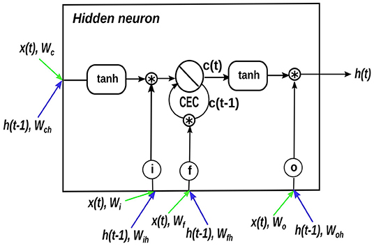
Figure 1. A LSTM hidden neuron. i, f, and o represent the input, forget, and output gates, which are activated by the sigmoid function. The green arrows indicate the entry of new inputs into the hidden neuron, and the blue arrows show the entry of neuron outputs of the previous time step (i.e., t – 1) into the hidden neuron. For the sake of simplicity, biases are not shown here.

Given an input variable whose time series is x(t) (t ≥ 1), the computing process in a LSTM hidden neuron (Figure 1) at the time step t is presented by Eqs 1–6.

$\begin{array}{ll}i(t)=\sigma (w_{i}x(t)+b_i+w_{ih}h(t-1)+b_{ih})& (1)\end{array}$

$\begin{array}{ll}f(t)=\sigma (w_{f}x(t)+b_f+w_{fh}h(t-1)+b_{fh})& (2)\end{array}$

$\begin{array}{ll}o(t)=\sigma (w_{o}x(t)+b_o+w_{oh}h(t-1)+b_{oh})& (3)\end{array}$

$\begin{array}{ll}g(t)=tanh(w_{c}x(t)+b_c+w_{ch}h(t-1)+b_{ch})& (4)\end{array}$

$\begin{array}{ll}c(t)=f{(t)}^{*}c(t-1)+i{(t)}^{*}g(t)& (5)\end{array}$

$\begin{array}{ll}h(t)=o{(t)}^{*}tanh(c(t))& (6)\end{array}$

where, i(t), f(t), o(t) are the information that enters into the neuron via the input, forget and output gates, respectively; h(t − 1) and h(t) are the neuron output at time step t – 1 and t, respectively; c(t − 1) and c(t) are the cell state at time step t – 1 and t, respectively; $w_{{}^{*}}$ and $b_{{}^{*}}$ are the learnable weight and bias on a linkage between neurons, respectively, and the subscripts i, f, o and c represent the input, forget and output gates and the cell state, respectively, e.g., w_i is the weight on the linkage of the new input x(t) to the input gate of a hidden neuron while w_ih is the weight on the linkage of the previous neuron output h(t − 1) to the input gate of a hidden neuron; σ represents the sigmoid function; tanh represents the hyperbolic tangent function; * represents the Hadamard product.

At the individual pixel level, we constructed one-hidden-layer LSTM networks, due to the relatively small amount of data available (i.e., a total of 252 time steps). The numbers of neurons on the input and output layers depend on the numbers of input and output variables, respectively, and they are constant in each experiment. Therefore, in this study, the network complexity is only affected by the number of hidden neurons, which is the only hyperparameter to tune during network validation (described in Section Experimental Design). The desired number of hidden neurons should allow a network not only to gain enough knowledge from a given data set but also be able to handle previously unobserved data (Dawson and Wilby, 2001; Müller and Guido, 2017).

Wavelet Coherence Analysis

Wavelet transforms map time series into the time-frequency domain and help localizing intermittent periodicities. Continuous wavelet transform is a common type of wavelet transforms useful for feature extraction (Grinsted et al., 2004). The continuous wavelet transform of a discrete time series x_n0 at the time step n and a specific time scale s is given by Eq. 7.

$\begin{array}{ll}W(s,n)={\displaystyle \sum _{n_0=0}^{N-1}}{x}_{n_0}{\psi }^{*}\left[\frac{(n_0-n)\delta t}{s}\right]& (7)\end{array}$

where, ψ is the mother wavelet, here using the Morlet wavelet, and ψ^* is the complex conjugate of ψ; δt is the time step of x_n0; N is the total number of δt in x_n0. The power of the continuous wavelet transform is defined as |W(s, n)|² (Torrence and Compo, 1998). While continuous wavelet transform can effectively identify localized intermittent oscillations in the time-frequency domain, it is only applicable to a single time series.

Wavelet coherence analysis is a method that measures the cross-correlation of two time-dependent variables in the time-frequency domain, of which calculation (Eq. 8) is based on continuous wavelet transform. The results of wavelet coherence analysis are comparable with traditional correlation coefficients, ranging from 0 to 1.

$\begin{array}{ll}Coherence(s,n)=\frac{|\langle s^{-1}{W}_{xy}(s,n)\rangle {|}^2}{\langle s^{-1}|W_x(s,n){|}^2\rangle \langle s^{-1}|W_y(s,n){|}^2\rangle }& (8)\end{array}$

where, the 〈 • 〉 indicates smoothing in both time and scale; W_x(s, n) and W_y(s, n) are the continuous wavelet transforms of the time series x_n0 and y_n0; W_xy(s, n) is the cross-wavelet spectrum of the time series x_n0 and y_n0 and equal to $W_x(s,n)W_y^{*}(s,n)$, and the (*) indicates the complex conjugate (Torrence and Webster, 1999; Grinsted et al., 2004).

The phase shift in the results of wavelet coherence analysis is calculated by:

$\begin{array}{ll}\varphi (s,n)={\text{tan}}^{-1}(\Im \left\{\langle s^{-1}{W}_{xy}(s,n)\rangle \right\}/\Re \left\{\langle s^{-1}{W}_{xy}(s,n)\rangle \right\})& (9)\end{array}$

where, ℑ{ • } and ℜ{ • } signify the imaginary and real parts of a complex number, respectively (Torrence and Webster, 1999). ϕ(s, n) = 0 means that the wavelets of two considered time series at the time step n and the time scale s are in phase. Detailed descriptions of wavelet coherence analysis and phase shift can be found in Torrence and Webster (1999), Grinsted et al. (2004) and Rahmati et al. (2020).

In this study, we conducted wavelet coherence analysis to derive the time-frequency correlation and phase shifts between regionally averaged wtd_a time series obtained from the TSMP-G2A data set and the LSTM network results. In this way, we expected to gain an understanding of the network performance in various experiments and thus help explain the contributions of different input variable combinations to the estimation of wtd_a over Europe in the time-frequency domain.

Study Area and Data Set

We utilized the TSMP-G2A data set to evaluate the ability of the proposed LSTM networks to estimate wtd_a over Europe in different experiments. As aforementioned, the dataset contains daily averaged continuous simulation results over Europe from TSMP, which is a fully coupled atmosphere-land-surface-subsurface modeling system. The spatial resolution of the dataset is 0.11° (~12.5 km). For details regarding TSMP and the TSMP-G2A data set, the reader is referred to Gasper et al. (2014); Shrestha et al. (2014) and Furusho-Percot et al. (2019).

This study focused on eight different European regions, which are known as the PRUDENCE regions (Christensen and Christensen, 2007): Scandinavia (SC), British Isles (BI), Mid-Europe (ME), Eastern Europe (EA), France (FR), Alps (AL), Iberian Peninsula (IB), and Mediterranean (MD). The individual PRUDENCE regions are characterized by different hydrometeorological regimes, potentially resulting in various responses of groundwater anomalies to other hydrometeorological variables, and constitute reference regions in climate science. Regionally averaged precipitation, evapotranspiration and soil moisture values calculated from the TSMP-G2A data set range from 776 mm (EA) to 1,494 mm (AL), 283 mm (SC) to 518 mm (MD) and 0.29 m³m⁻³ (IB) to 0.36 m³m⁻³ (BI), respectively. Regionally averaged wtd values are from 2 m to 3 m, apart from AL (4.14 m), IB (6.62 m) and MD (6.48 m). Figure 2 presents the yearly averaged spatially distributed wtd values calculated from the TSMP-G2A data set from 01/1996 to 12/2016. Based on intervals of yearly averaged wtd, we categorized pixel values into three classes following Ma et al. (2021), that is, C1 corresponding to 0.0 m < wtd ≤ 3.0 m, C2 corresponding to 3.0 m < wtd ≤ 10.0 m and C3 corresponding to wtd > 10.0 m. Most pixels on the European continent belong to C1 (colored in light blue), accounting for 52% to 75% of different PRUDENCE regions. <20% of pixels in each PRUDENCE region belong to C2 (colored in orange). <15% of pixels in each PRUDENCE region belong to C3 (colored in red), except for AL (24%), IB (30%) and MD (28%). In addition, there is also a heterogeneous pattern in the yearly averaged snow water equivalent (SWE) values (not shown here) derived from the TSMP-G2A data set. SC and AL have the largest regionally averaged SWE (>60 mm) while the other regions have regionally averaged SWE < 10 mm.

FIGURE 2

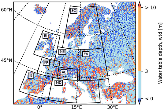
Figure 2. TSMP-G2A wtd [m] climatology over the European continent from 01/1996 to 12/2016. Areas bounded by the black polygons show PRUDENCE regions (i.e., SC, Scandinavia; BI, British Isles; ME, Mid-Europe; EA, Eastern Europe; FR, France; AL, Alps; IB, Iberian Peninsula; MD, Mediterranean).

The anomaly data were calculated from the TSMP-G2A data set for each calendar month and pixel individually for the period 01/1996 to 12/2016 to enable the spatial comparability and to account for the seasonality in the variables. Here, we only considered the data after the year 1996 to avoid the influence of spinup effects on the simulation results (Furusho-Percot et al., 2019). We used Eq. 10 to calculate pr_a, ET_a, θ_a and wtd_a, where the climatological average and standard deviation values were derived from the training set (i.e., the data from 01/1996 to 12/2012, described in Section Experimental Design) to prevent future information from leaking into the training process. rs_a = wtd_a at pixels where wtd ≤ 0 m. Regionally averaged pr_a, ET_a, θ_a and wtd_a time series for the wtd categories C1 to C3 in different PRUDENCE regions are presented in Supplementary Figure 1.

$\begin{array}{ll}{v}_a=(v_m-v_{av})/v_{sd}& (10)\end{array}$

where, v is the considered variable, such as wtd; v_m is the monthly data of v calculated from the TSMP-G2A data set; v_av is the climatological average of v_m (i.e., averages of v_m in January, February, …, December); v_sd is the climatological standard deviation of v_m.

pr_a, ET_a, θ_a, rs_a and wtd_a are measures of different types of drought. Table 1 provides the definition of drought severity based on anomalies, following McKee et al. (1993).

TABLE 1

Table 1. Definition of drought severity based on anomalies.

Moreover, we utilized Eqs 11, 12 to calculate SWE_scaled from SWE which has data only available from 01/2003 to 12/2010. The obtained SWE_scaled data only has one value in the range from −1 to 1 at each pixel, so it is static.

$\begin{array}{ll}SW{E}_0=(SW{E}_y-SW{E}_{min})/(SW{E}_{max}-SW{E}_{min})& (11)\end{array}$

$\begin{array}{ll}SW{E}_{scaled}=SW{E}_0*\left[1-(-1)\right]+(-1)& (12)\end{array}$

where, SWE_y is the yearly averaged SWE value from 2003 to 2010; SWE_min is the minimum value of SWE_y over the European continent; SWE_max is the maximum value of SWE_y over the European continent.

Experimental Design

In this study, we varied a number of input variables, in addition to pr_a used in the LSTM networks proposed in Ma et al. (2021), to arrive at improved wtd_a estimates. The combinations of input variables used in different experiments are listed in Table 2. We selected the input variables based on their demonstrated relationship with wtd_a (Van Loon, 2015) and availability in the TSMP-G2A data set and common observational datasets. In E1, the LSTM networks used combinations of pr_a, ET_a and θ_a as input. pr_a, ET_a and θ_a are drought-related hydrometeorological variables with spatiotemporally continuous data over Europe, which can be easily obtained from observations and reanalysis datasets, e.g., ERA5-Land. pr_a and ET_a are measures of meteorological drought, while θ_a shows the degree of agricultural drought. Except for the input variables involved in E1, the quality of wtd_a estimates can also be affected by SWE; Ma et al. (2021) found that large SWE can degrade the network test performance. Moreover, in an unconfined aquifer, groundwater and surface water dynamics have a strong lateral connection, and thus, wtd_a at a pixel is also influenced by the change in water dynamics at neighboring pixels, especially for a pixel close to a river, due to the interaction between surface water and groundwater. Here, in addition to the optimal input variable combination determined in E1, we introduced a static input SWE_scaled and anomalies at adjacent pixels as input to the LSTM networks in E2, to explore potential improvement in the network performance. Especially, at pixels close to rivers, we investigated the impact of rs_a at adjacent pixels on the network performance (see E2.3).

TABLE 2

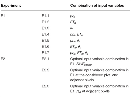
Table 2. Combinations of input variables in different experiments.

At the individual pixel level, we divided anomaly data into a training set (01/1996–12/2012, 204 time steps, about 80% of the total data), a validation set (01/2013–12/2014, 24 time steps, about 10% of the total data) and a test set (01/2015–12/2016, 24 time steps, about 10% of the total data) for network training, validation and testing, respectively. The static input SWE_scaled provided the same value at every time step.

The LSTM networks applied here have the same configuration of hyperparameters (listed in Table 3) as Ma et al. (2021), except for the number of input neurons which depends on the number of input variables used in the different experiments. As described in Section Long Short-Term Memory Networks, the number of hidden neurons has a significant impact on the network performance and is the only hyperparameter to tune here, ranging from 1 to 100.

TABLE 3

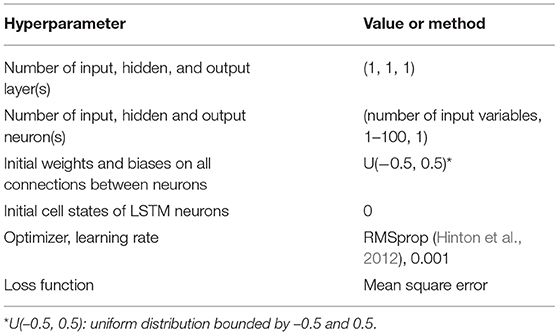
Table 3. Hyperparameter setting of the applied LSTM networks [adopted from Ma et al. (2021)].

Figure 3 illustrates the generic workflow used to construct the LSTM networks at the individual pixel level in the different experiments. The workflow started with the network training process during which we fitted the training set to the LSTM networks with 1 to 100 hidden neurons. An epoch is an iteration when the whole training set travels once through the network forward and backward. Weights and biases on all connections between neurons commenced from random values selected from a uniform distribution bounded by −0.5 and 0.5, and in each epoch, the networks automatically updated weights and biases based on the difference between the network output and the target data (i.e., TSMP-G2A wtd_a) calculated by the loss function (here Mean Square Error). The technique of adjusting weights and biases is termed an optimizer (here RMSprop), and the rate at which an optimizer adjusts weights and biases is termed learning rate (here 0.001). In the interval of two consecutive epochs, the network validation process was run to check the performance of the trained network in each epoch on the validation set. The criteria for stopping the training process were (1) the number of epochs ≥50; and (2) the validation performance started to decrease. Based on the validation performance, we determined three optimal numbers of hidden neurons, which were often various for the LSTM networks constructed at different pixels. In the end, we applied the trained networks with the three optimal numbers of hidden neurons on the test set (i.e., unobserved data during training) and averaged the results from the three networks as the final result for evaluation. In this way, we compensated for the individual shortcomings of the selected networks to some extent and obtained improved final results. For details about the network setup, the reader is referred to Ma et al. (2021).

FIGURE 3

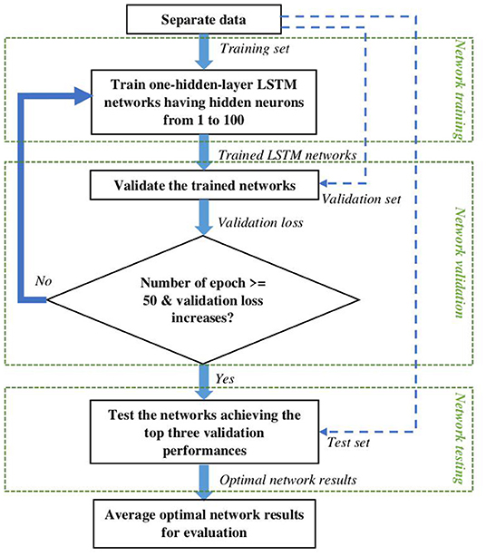
Figure 3. A generic workflow to construct the LSTM networks at individual pixels [adopted from Ma et al. (2021)]. The blue dashed lines with arrows represent data transmission paths.

We adopted RMSE and R² as the metrics to assess the network performance, which show the goodness of fit of the LSTM networks in terms of the magnitude and variance of the error. They are calculated by Eqs 13, 14, and the LSTM networks having good performance are expected to obtain low RMSEs and high R² scores.

$\begin{array}{ll}RMSE=\sqrt{{\displaystyle \sum _{i=1}^N}{(y_t-y_m)}^2/N}& (13)\end{array}$

$\begin{array}{ll}{R}^2=1-{\displaystyle \sum _{i=1}^N}{(y_t-y_m)}^2/{\displaystyle \sum _{i=1}^N}{(y_t-\overline{y_t})}^2& (14)\end{array}$

where, y_t and $\overline{y_t}$ are the target value (i.e., TSMP-G2A wtd_a) and the average of the target values, respectively; y_m is the modeled value (i.e., the network output, hereafter named LSTM wtd_a); N is the number of time steps in the given time series.

To save computational resources, we constructed the LSTM networks locally at a limited number of pixels, which were randomly selected in each PRUDENCE region. Ma et al. (2021) found that yearly averaged wtd considerably affected the test performance of the LSTM networks with pr_a as input, and for increasing wtd, the networks tended to behave poorly. Hence, during the analyses of the network results (presented in Section Results), we separated the selected pixels in each PRUDENCE region into the wtd categories C1 to C3 based on their wtd values.

Results

Test Performance of the LSTM Networks in the Different Experiments

We aimed to identify the LSTM networks with the best test performance in the designed experiments in handling previously unobserved data. Figures 4, 5 illustrate the box plots of the test R² scores and RMSEs achieved by the LSTM networks in the different experiments at the selected pixels belonging to the wtd categories C1 to C3 in each PRUDENCE region, respectively. For a better visualization, we set negative R² scores to zero in Figure 4. The medians of the test R² and RMSEs achieved in different experiments for C1 to C3 in each PRUDENCE region are listed in Supplementary Table 1.

FIGURE 4

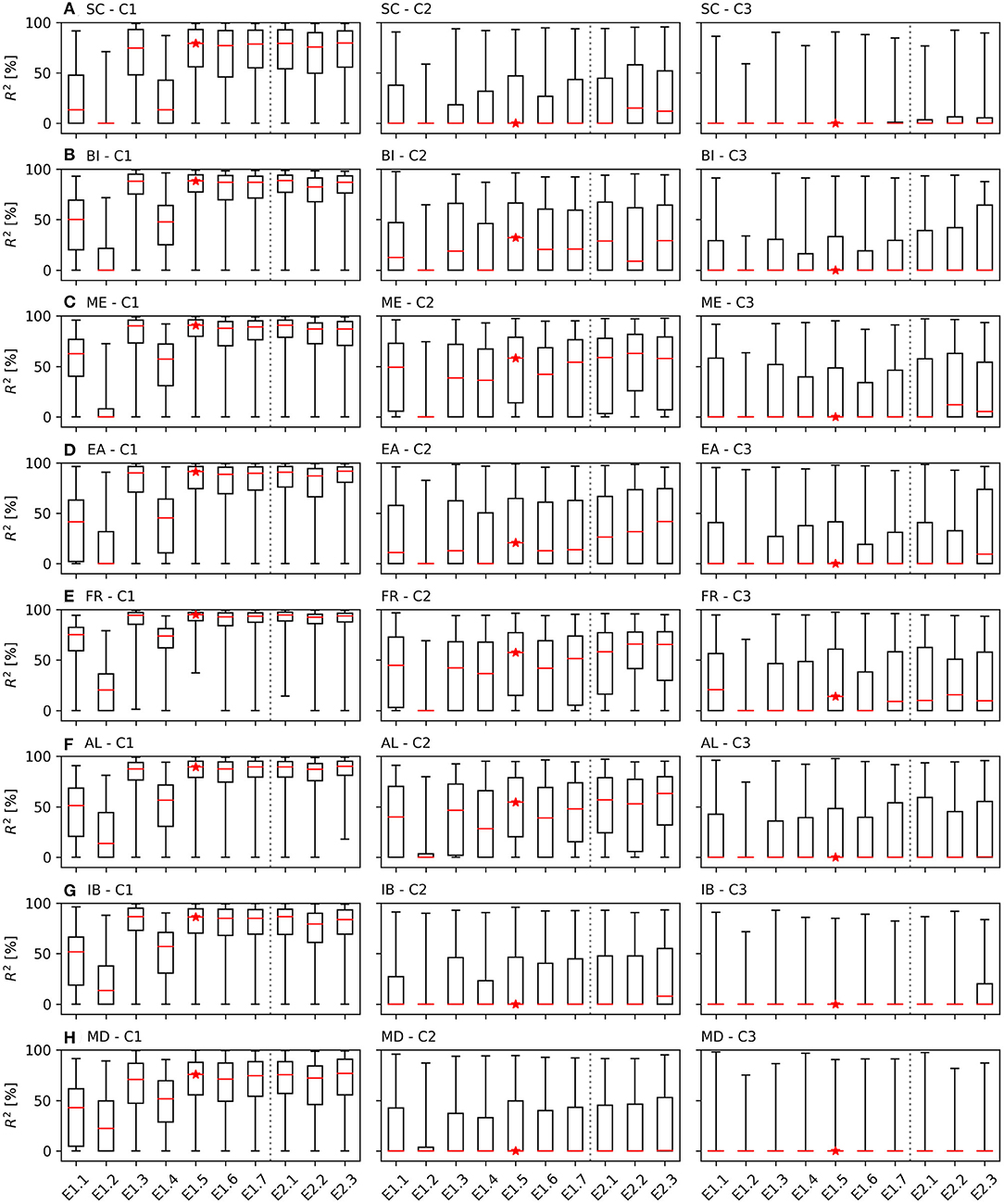
Figure 4. Box plots of test R² scores achieved by the LSTM networks of E1 and E2: E1.1: pr_a; E1.2: ET_a; E1.3: θ_a; E1.4: pr_a and ET_a; E1.5: pr_a and θ_a; E1.6: ET_a and θ_a; E1.7: pr_a, ET_a and θ_a; E2.1: pr_a, θ_a and SWE_scaled; E2.2: pr_a, θ_a at the selected pixels and adjacent pixels; and E2.3: pr_a, θ_a at the selected pixels close to rivers and rs_a at the adjacent pixels. (A–H) show the comparison of the box plots at the selected pixels belonging to the wtd categories C1 to C3 in each PRUDENCE region. The box plots show the ranges of the R² scores from the first quartile to the third quartile; the red lines indicate the medians of the R² scores; and the upper and lower ends represent the maximum and minimum values of the R² scores, respectively. The medians of the R² scores obtained by the LSTM networks of E1.5 are marked with red stars. The box plots for E1 and E2 are separated by gray dotted lines.

FIGURE 5

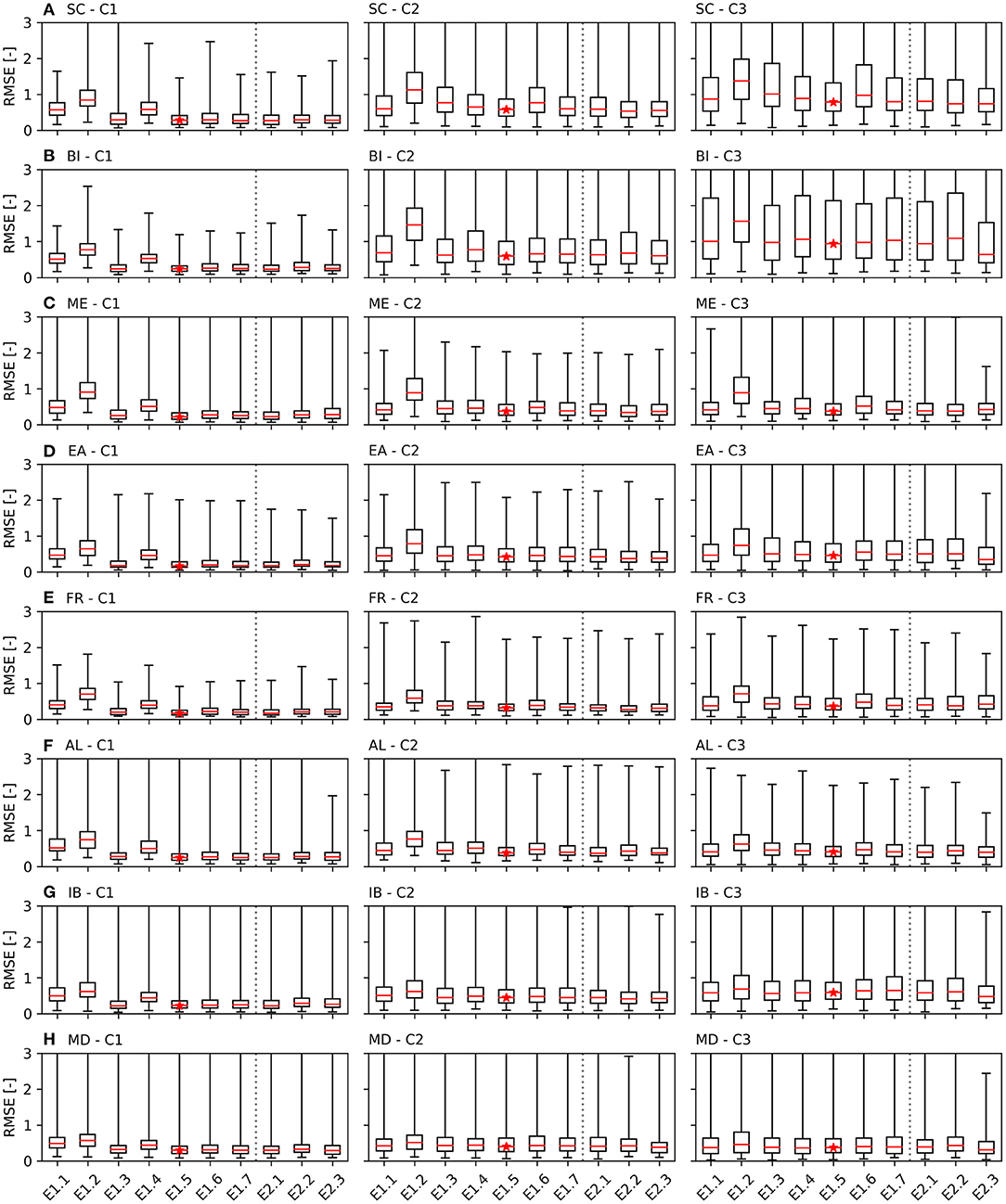
Figure 5. Box plots of test RMSEs achieved by the LSTM networks of E1 and E2. (A–H) show the comparison of the box plots at the selected pixels belonging to the wtd categories C1 to C3 in each PRUDENCE region. The labels have the same definitions as Figure 4, but for RMSEs.

The LSTM networks of E1.5 (marked with red stars in Figures 4, 5) achieved the optimal test performance not only in E1 but also in all the designed experiments, which used pr_a and θ_a as input. They obtained the test scores as follows: median R² of 76–95% for C1, 0–58% for C2, and 0–14% for C3; and median RMSEs of 0.17–0.30 for C1, 0.32–0.60 for C2, and 0.36–0.94 for C3. The evaluation metrics were significantly improved compared to those obtained by the LSTM networks employed in Ma et al. (2021), particularly for C1 (with a 20–66% increase in median R² and a 0.19–0.30 decrease in median RMSEs), which is the major wtd category in Europe. Over Europe, the LSTM networks of E1.5 showed good test performance with a test R² score ≥ 50% at most selected pixels (Figure 6). In addition, Table 4 gives close to or over half of the selected pixels with a test R² score ≥50% in the PRUDENCE regions for the LSTM networks of E1.5, constituting an increase of 8 to 22% compared to Ma et al. (2021). The highly improved wtd_a estimates by including θ_a as input suggest that θ_a plays an important role in explaining groundwater dynamics over Europe. One possible reason for that is, compared with pr_a and ET_a, θ_a provides more information about subsurface hydrological processes, such as vegetation influence, soil heterogeneity and, thus, varying infiltration and recharge rates. Because θ_a and wtd_a are measures of agricultural drought and groundwater drought, respectively, the substantial contribution of θ_a to wtd_a also suggests the close connection between agricultural drought and groundwater drought over Europe.

FIGURE 6

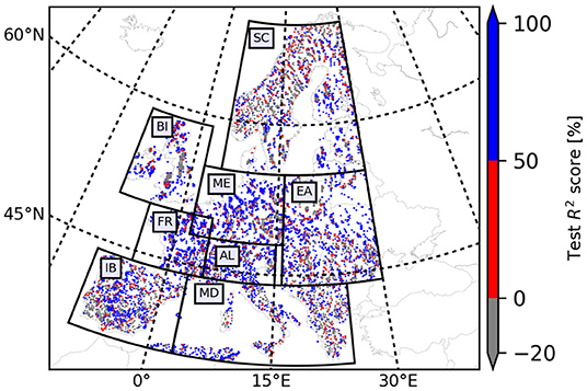
Figure 6. Map of test R² scores achieved by the LSTM networks of E1.5 (pr_a and θ_a) in the PRUDENCE regions.

TABLE 4

Table 4. Percentages of the selected pixels with a test R² score ≥50% in the PRUDENCE regions (%) for the LSTM networks of E1.5.

In E2.1, no noticeable improvement was detected in the test R² scores and RMSEs especially in SC and AL that have large SWE (see Figures 4, 5) by adding SWE_scaled as additional input to the LSTM networks of E1.5, implying little additional contribution of snow accumulation to the estimation of wtd_a over Europe. This seems to be inconsistent with the conclusion of Ma et al. (2021) that SWE strongly affects the quality of wtd_a estimates. However, the discrepancy can be explained by the fact that soil moisture is partly replenished by snow water and thus θ_a already includes information about SWE.

In Figures 4, 5, we found that only the test R² scores and RMSEs for the wtd categories C2 and C3 (wtd > 3.0 m) were partially improved by adding anomalies available at neighboring pixels as input to the LSTM networks of E1.5 (i.e., E2.2 and E2.3). It indicates the lateral exchange of groundwater mainly influences groundwater dynamics in deep aquifers. The improvement was small (<0.1 for median RMSEs) for C2 and C3, and the network test performance was generally degraded for C1 to which more than half of the pixels over Europe belong, and thus, the LSTM networks of E2.2 and E2.3 are expected to gain worse test performance compared to the LSTM networks of E1.5 at the European scale.

In general, Figures 4, 5 show the decrease in network test performance with increasing average wtd (from C1 to C3), manifested in the smaller medians of test R² scores and larger medians of test RMSEs, which is in good agreement with the finding in Ma et al. (2021). Moreover, we also found only small contributions of ET_a to the estimation of wtd_a at the European scale compared to other drought-related input variables reflected in the worst test performance in E1.2 (ET_a).

European Water Table Depth Anomaly Map in 2015 Reproduced by the Results of the Optimal LSTM Networks

In 2015, large parts of the European continent were affected by an extreme summer heatwave, causing severe drought (Van Loon et al., 2017). Here, based on the results of the optimal LSTM networks (E1.5: pr_a and θ_a), we reproduced the European wtd_a map derived from the TSMP-G2A data set for August 2015 (Figure 7), which was one of the driest months in 2015. The study month is in the testing period, and thus, the networks have not seen the data during training. Nevertheless, the reproduced map is in good agreement with the original map (Figure 7) concerning drought severity through a visual inspection. Both show the spatially heterogeneous distribution of wtd_a over Europe, including the strong groundwater anomalies (wtd_a ≥ 1.5) in ME, EA, and AL and the very wet conditions (wtd_a ≤ −1.5) in SC and BI, which is consistent with previous studies (e.g., Dong et al., 2016; Van Lanen et al., 2016; Van Loon et al., 2017). Moreover, the optimal LSTM networks successfully detected ~41% of strong drought events (wtd_a ≥ 1.5) and ~29% of extreme drought events (wtd_a ≥ 2) at the European scale in August 2015, outperforming the original LSTM networks proposed in Ma et al. (2021), (E1.1, Supplementary Figure 2B) with the hit rates only ~15% for strong drought events and ~3% for extreme drought events.

FIGURE 7

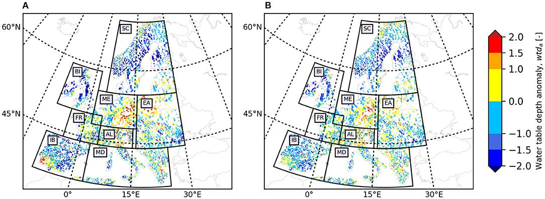
Figure 7. European wtd_a maps for August 2015 (i.e., in the testing period), derived from (A) the TSMP-G2A data set and (B) results from the LSTM networks of E1.5 (pr_a and θ_a).

Wavelet Coherence Analysis on Regionally Averaged Water Table Depth Anomaly Time Series in ME

The significantly improved test performance of the LSTM networks of E1.5 is attributed to information contained in θ_a for estimating certain frequency components of wtd_a. Therefore, here we conducted wavelet coherence analysis on the regionally averaged wtd_a time series for the wtd categories C1 to C3 in ME (Figure 8), which were derived from the TSMP-G2A data set and the LSTM network results in E1.1 and E1.5. We focused on the areas within the black dashed lines to eliminate edge effects and to gain a better understanding of the contribution of θ_a on the explanation of groundwater anomalies in the time-frequency domain.

FIGURE 8

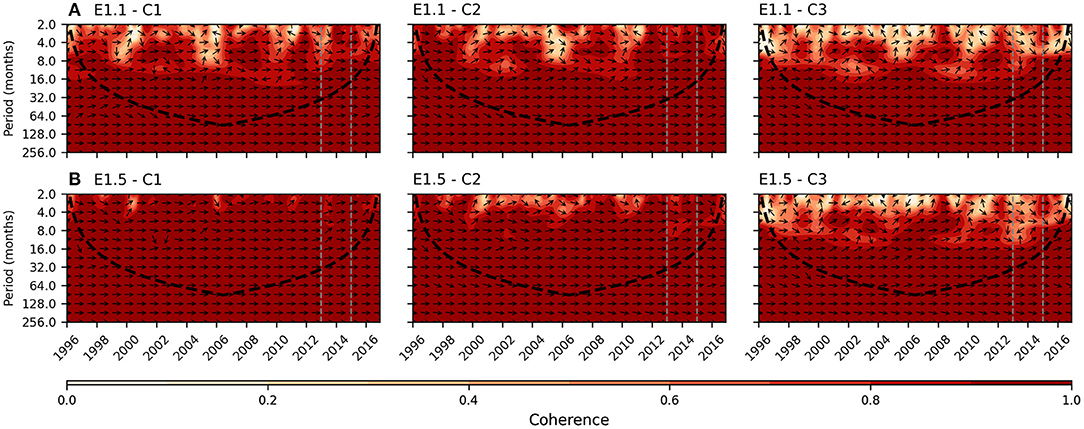
Figure 8. Results of wavelet coherence analysis on the regionally averaged wtd_a time series for the wtd categories C1 to C3 in ME, which were derived from the TSMP-G2A data set and the results of the LSTM networks of: (A) E1.1: pr_a; and (B) E1.5: pr_a and θ_a. The training, validation and testing periods are separated by gray dashed lines.

By introducing θ_a as additional input, the coherence between the regionally averaged wtd_a time series was significant improved at periods between 2 and 8 months, especially for the wtd categories C1 and C2, revealing the larger contribution of θ_a to explain groundwater dynamics at the monthly and seasonal cycles compared to pr_a. Moreover, in Figure 8B, most phase shifts at periods between 2 and 8 months are zero for the wtd categories C1, suggesting almost no time lag between the modeled and target regionally averaged wtd_a time series in shallow aquifers of ME. The similar conclusions can also be drawn from the results of wavelet coherence analysis in other PRUDENCE regions, which are shown in Supplementary Figures 3–9.

Discussion

The scarcity of wtd observations complicates groundwater monitoring and requires alternative methods to quantify or predict wtd_a. The pr_a is the most common proxy of wtd_a, mainly due to the close connection between meteorological and groundwater droughts and the easy access to global precipitation data. This study, however, showed the limits of merely using pr_a and/or ET_a data to estimate wtd_a over Europe. Similar conclusions were also drawn by e.g., Kumar et al. (2016), Uddameri et al. (2019), who compared the performance of the Standardized Precipitation Index over extended time scales to quantify groundwater drought with the Standardized Groundwater level Index. One potential reason is that the occurrence of groundwater drought depends not only on the precipitation and temperature anomalies but also on the antecedent water storage (Van Lanen et al., 2016). Therefore, including ground-based information such as θ_a significantly improved the network results in the presented study. In addition, similar to precipitation, soil moisture data is available from e.g., remotely sensed observations and reanalysis products, which removes the barriers to using θ_a as input for estimating wtd_a in real world applications.

The 2015 European summer heatwave started in June and resulted in peak temperatures in early July (Dong et al., 2016). Because most aquifers in Europe are shallow (with simulated wtd ≤ 3 m), a rapid response of groundwater was noticed, and the groundwater drought was already severe in several parts of Europe in August 2015. Although the impact of the groundwater drought continued until the end of 2015 (not shown here), its affected area was much smaller than the meteorological drought in the same year (Dong et al., 2016; Van Lanen et al., 2016). This indicates that not all meteorological droughts will evolve into groundwater droughts, and thus simply considering precipitation information is not enough to quantify groundwater drought, which is consistent with our previous observation. Moreover, the locations with groundwater drought coincided well with those with vegetation stress presented in Van Lanen et al. (2016), which also confirms the usefulness of soil moisture information in the estimation of groundwater anomalies.

The wavelet coherence analysis helped to explain the added value of θ_a as input in the estimation of wtd_a from the time-frequency perspective. Considering θ_a consistently increased the coherence between regionally averaged TSMP-G2A and LSTM wtd_a time series at periods between 2 and 8 months. This reflects the systematic contribution of θ_a to the explanation of groundwater anomalies.

Temporal Convolutional Networks (Yan et al., 2020) and Transformers (Vaswani et al., 2017) may constitute alternatives to the LSTM networks proposed here, which have been shown to outperform LSTM networks in handling long time series. The estimation of groundwater anomalies in deep aquifers may benefit from the application of these methods. Yet, in the simulations, most aquifers in Europe have yearly averaged wtd value ≤ 3 m, in which the response of wtd_a to hydrometeorological variables is expected to be relatively fast. Therefore, the improvement achieved by these methods may be not significant compared to LSTM networks.

Summary and Conclusions

In this study, we conducted several experiments to investigate the impacts of additional input variable combinations in the LSTM networks proposed in Ma et al. (2021) to improve monthly wtd_a estimates at individual pixels in eight hydrometeorologically different regions over Europe (i.e., PRUDENCE regions). Except for the original input variable pr_a, we introduced ET_a, θ_a, SWE_scaled, and anomalies at adjacent pixels (e.g., rs_a, see Table 2) as optional input variables to the LSTM networks. All assessments were based on anomalies derived from the TSMP-G2A data set, which contains daily integrated hydrologic simulation results over the European continent.

Because R² scores and RMSEs only provide limited information on the network performance, we also applied wavelet coherence analysis to investigate the contribution of the input variable(s) to explain groundwater anomalies over Europe in the time-frequency domain.

The optimal LSTM networks were found with pr_a and θ_a as input. Considering θ_a strongly improved the network test performance particularly in the areas with wtd ≤ 3 m (i.e., the major wtd category), suggesting that θ_a plays a significant role in the estimation of wtd_a over Europe. Because θ_a is related to agricultural drought and wtd_a shows the degree of groundwater drought, we conclude that a strong link exists between agricultural drought and groundwater drought on the European continent. The proposed LSTM networks can generate good results in shallow aquifers but may fail in deep aquifers. Therefore, one should be careful to use such networks in areas with large wtd.

We recognize that the network performance was limited by the relatively small amount of available training data, the simplified tuning of hyperparameters, and the application of simulation data (i.e., the TSMP-G2A data set) for evaluation. The biases of the TSMP-G2A dataset mainly come from uncalibrated parameters and neglect of human impacts (Furusho-Percot et al., 2019). Nevertheless, due to the good agreement of the TSMP-G2A data set with hydrological observational datasets, we argue that the methodology is useful in determining the optimal input variable combination for the estimation of wtd_a over Europe. Our study highlights the benefit in combining soil moisture information with precipitation information to estimate wtd_a over Europe. The input of the LSTM networks should have valid values continuous in time. In the future, the indirect method based on the optimal LSTM networks may be transferred to real-time monitoring of groundwater drought at the European scale using remotely sensed surface soil moisture observations from e.g., the SMOS (Kerr et al., 2010) and SMAP (Entekhabi et al., 2010) missions and precipitation observations from e.g., the GPM (Hou et al., 2014) and TRMM (Huffman et al., 2007) missions. Similarly, also some numerical weather prediction models provide the necessary variables, e.g., the ECMWF Integrated Forecasting System with assimilated ASCAT (MetOp Advanced SCATerometer) soil moisture data (Aires et al., 2021).

Data Availability Statement

The raw data supporting the conclusions of this article will be made available by the authors, without undue reservation.

Author Contributions

YM conceived and designed the experiments with the support of SK. YM conducted all the experiments and analyzed the results with feedback from CM, BB, and SK. YM prepared the manuscript with contributions from all co-authors. All authors contributed to the article and approved the submitted version.

Funding

This work was supported by the European Commission HORIZON 2020 Program ERA-PLANET/GEOEssential project (grant number: 689443).

Conflict of Interest

The authors declare that the research was conducted in the absence of any commercial or financial relationships that could be construed as a potential conflict of interest.

Publisher's Note

All claims expressed in this article are solely those of the authors and do not necessarily represent those of their affiliated organizations, or those of the publisher, the editors and the reviewers. Any product that may be evaluated in this article, or claim that may be made by its manufacturer, is not guaranteed or endorsed by the publisher.

Acknowledgments

The authors gratefully acknowledge the computing time granted through JARA-HPC and the VSR commission on the supercomputer JUWELS at Forschungszentrum Jülich.

Supplementary Material

The Supplementary Material for this article can be found online at: https://www.frontiersin.org/articles/10.3389/frwa.2021.723548/full#supplementary-material

Abbreviations

pr_a, precipitation anomaly; ET_a, evapotranspiration anomaly; rs_a, river stage anomaly; θ_a, soil moisture anomaly; wtd_a, water table depth anomaly; wtd, water table depth; LSTM networks, Long Short-Term Memory networks; TSMP, Terrestrial Systems Modeling Platform; SWE_scaled, scaled yearly averaged snow water equivalent; SWE, snow water equivalent.

References

Aires, F., Weston, P., de Rosnay, P., and Fairbairn, D. (2021). Statistical approaches to assimilate ASCAT soil moisture information—I. Methodologies and first assessment. Q. J. R. Meteorol. Soc. 147, 1823–1852. doi: 10.1002/qj.3997

CrossRef Full Text | Google Scholar

Bachmair, S., Tanguy, M., Hannaford, J., and Stahl, K. (2018). How well do meteorological indicators represent agricultural and forest drought across Europe? Environ. Res. Lett. 13:034042. doi: 10.1088/1748-9326/aaafda

CrossRef Full Text | Google Scholar

Bloomfield, J. P., and Marchant, B. P. (2013). Analysis of groundwater drought building on the standardised precipitation index approach. Hydrol. Earth Syst. Sci. 17, 4769–4787. doi: 10.5194/hess-17-4769-2013

CrossRef Full Text | Google Scholar

Brauns, B., Cuba, D., Bloomfield, J. P., Hannah, D. M., Jackson, C., Marchant, B. P., et al. (2020). The Groundwater Drought Initiative (GDI): analysing and understanding groundwater drought across Europe. Proc. Int. Assoc. Hydrol. Sci. 383, 297–305. doi: 10.5194/piahs-383-297-2020

CrossRef Full Text | Google Scholar

Christensen, J. H., and Christensen, O. B. (2007). A summary of the PRUDENCE model projections of changes in European climate by the end of this century. Clim. Change 81, 7–30. doi: 10.1007/s10584-006-9210-7

CrossRef Full Text | Google Scholar

Dawson, C. W., and Wilby, R. L. (2001). Hydrological modelling using artificial neural networks. Prog. Phys. Geogr. 25, 80–108. doi: 10.1177/030913330102500104

CrossRef Full Text | Google Scholar

Dong, B., Sutton, R., Shaffrey, L., and Wilcox, L. (2016). The 2015 European heat wave. Bull. Am. Meteorol. Soc. 97, S57–S62. doi: 10.1175/BAMS-D-16-0140.1

CrossRef Full Text | Google Scholar

Entekhabi, D., Njoku, E. G., O'Neill, P. E., Kellogg, K. H., Crow, W. T., Edelstein, W. N., et al. (2010). The soil moisture active passive (SMAP) mission. Proc. IEEE 98, 704–716. doi: 10.1109/JPROC.2010.2043918

CrossRef Full Text | Google Scholar

European Environment Agency (2020). Meteorological and Hydrological Droughts in Europe. Available online at: https://www.eea.europa.eu/data-and-maps/indicators/river-flow-drought-3/assessment (accessed July 7, 2020).

Fang, Z., Bogena, H., Kollet, S., Koch, J., and Vereecken, H. (2015). Spatio-temporal validation of long-term 3D hydrological simulations of a forested catchment using empirical orthogonal functions and wavelet coherence analysis. J. Hydrol. 529, 1754–1767. doi: 10.1016/j.jhydrol.2015.08.011

CrossRef Full Text | Google Scholar

Furusho-Percot, C., Goergen, K., Hartick, C., Kulkarni, K., Keune, J., and Kollet, S. (2019). Pan-European groundwater to atmosphere terrestrial systems climatology from a physically consistent simulation. Sci. Data 6:320. doi: 10.1038/s41597-019-0328-7

PubMed Abstract | CrossRef Full Text | Google Scholar

Gasper, F., Goergen, K., Shrestha, P., Sulis, M., Rihani, J., Geimer, M., et al. (2014). Implementation and scaling of the fully coupled terrestrial systems modeling platform (TerrSysMP v1.0) in a massively parallel supercomputing environment–a case study on JUQUEEN (IBM Blue Gene/Q). Geosci. Model Dev. 7, 2531–2543. doi: 10.5194/gmd-7-2531-2014

CrossRef Full Text | Google Scholar

Gers, F. A., Schmidhuber, J., and Cummins, F. (2000). Learning to forget: continual prediction with LSTM. Neural Comput. 12, 2451–2471. doi: 10.1162/089976600300015015

PubMed Abstract | CrossRef Full Text | Google Scholar

Grinsted, A., Moore, J. C., and Jevrejeva, S. (2004). Application of the cross wavelet transform and wavelet coherence to geophysical time series. Nonlinear Process. Geophys. 11, 561–566. doi: 10.5194/npg-11-561-2004

CrossRef Full Text | Google Scholar

Hänsel, S., Ustrnul, Z., Łupikasza, E., and Skalak, P. (2019). Assessing seasonal drought variations and trends over Central Europe. Adv. Water Resour. 127, 53–75. doi: 10.1016/j.advwatres.2019.03.005

CrossRef Full Text | Google Scholar

Hartick, C., Furusho-Percot, C., Goergen, K., and Kollet, S. (2021). An interannual probabilistic assessment of subsurface water storage over Europe using a fully coupled terrestrial model. Water Resour. Res. 57:e2020WR027828. doi: 10.1029/2020WR027828

CrossRef Full Text | Google Scholar

Hinton, G., Srivastava, N., and Swersky, K. (2012). Overview of Mini-Batch Gradient Descent. Available online at: https://www.cs.toronto.edu/~tijmen/csc321/slides/lecture_slides_lec6.pdf (accessed January 15, 2020).

Hochreiter, S., and Schmidhuber, J. (1997). Long short-term memory. Neural Comput. 9, 1735–1780. doi: 10.1162/neco.1997.9.8.1735

PubMed Abstract | CrossRef Full Text | Google Scholar

Hou, A. Y., Kakar, R. K., Neeck, S., Azarbarzin, A. A., Kummerow, C. D., Kojima, M., et al. (2014). The global precipitation measurement mission. Bull. Am. Meteorol. Soc. 95, 701–722. doi: 10.1175/BAMS-D-13-00164.1

CrossRef Full Text | Google Scholar

Huffman, G. J., Bolvin, D. T., Nelkin, E. J., Wolff, D. B., Adler, R. F., Gu, G., et al. (2007). The TRMM multisatellite precipitation analysis (TMPA): quasi-global, multiyear, combined-sensor precipitation estimates at fine scales. J. Hydrometeorol. 8, 38–55. doi: 10.1175/JHM560.1

CrossRef Full Text | Google Scholar

Kerr, Y. H., Waldteufel, P., Wigneron, J.-P., Delwart, S., Cabot, F., Boutin, J., et al. (2010). The SMOS mission: new tool for monitoring key elements ofthe global water cycle. Proc. IEEE 98, 666–687. doi: 10.1109/JPROC.2010.2043032

CrossRef Full Text | Google Scholar

Kratzert, F., Klotz, D., Brenner, C., Schulz, K., and Herrnegger, M. (2018). Rainfall–runoff modelling using long short-term memory (LSTM) networks. Hydrol. Earth Syst. Sci. 22, 6005–6022. doi: 10.5194/hess-22-6005-2018

CrossRef Full Text | Google Scholar

Kratzert, F., Klotz, D., Shalev, G., Klambauer, G., Hochreiter, S., and Nearing, G. (2019). Toward learning universal, regional, and local hydrological behaviors via machine learning applied to large-sample datasets. Hydrol. Earth Syst. Sci. 23, 5089–5110. doi: 10.5194/hess-23-5089-2019

CrossRef Full Text | Google Scholar

Kumar, R., Musuuza, J. L., Van Loon, A. F., Teuling, A. J., Barthel, R., Ten Broek, J., et al. (2016). Multiscale evaluation of the standardized precipitation index as a groundwater drought indicator. Hydrol. Earth Syst. Sci. 20, 1117–1131. doi: 10.5194/hess-20-1117-2016

CrossRef Full Text | Google Scholar

Labat, D. (2005). Recent advances in wavelet analyses: part 1. A review of concepts. J. Hydrol. 314, 275–288. doi: 10.1016/j.jhydrol.2005.04.003

CrossRef Full Text | Google Scholar

Lane, S. N. (2007). Assessment of rainfall-runoff models based upon wavelet analysis. Hydrol. Process. 21, 586–607. doi: 10.1002/hyp.6249

CrossRef Full Text | Google Scholar

Le, X. H., Ho, H. V., Lee, G., and Jung, S. (2019). Application of long short-term memory (LSTM) neural network for flood forecasting. Water (Switzerland) 11:1387. doi: 10.3390/w11071387

CrossRef Full Text | Google Scholar

Ma, Y., Matta, E., Meißner, D., Schellenberg, H., and Hinkelmann, R. (2019). Can machine learning improve the accuracy of water level forecasts for inland navigation?,” in Proceedings of the 38th IAHR World Congress (Panama). doi: 10.3850/38WC092019-0274

CrossRef Full Text

Ma, Y., Montzka, C., Bayat, B., and Kollet, S. (2021). Using long short-term memory networks to connect water table depth anomalies to precipitation anomalies over Europe. Hydrol. Earth Syst. Sci. 25, 3555–3575. doi: 10.5194/hess-25-3555-2021

CrossRef Full Text | Google Scholar

McKee, T. B., Doesken, N. J., and Kleist, J. (1993). “The relationship of drought frequency and duration to time scales,” in Proceedings of the 8th Conference on Applied Climatology (Anaheim), 179–184.

Google Scholar

Mishra, A. K., and Singh, V. P. (2010). A review of drought concepts. J. Hydrol. 391, 202–216. doi: 10.1016/j.jhydrol.2010.07.012

CrossRef Full Text | Google Scholar

Müller, A. C., and Guido, S. (2017). “Generalization, overfitting, and underfitting,” in Introduction to Machine Learning with Python: A Guide For Data Scientists, ed. D. Schanafelt (Sebastopol: O'Reilly Media, Inc.), 30.

Nalbantis, I., and Tsakiris, G. (2009). Assessment of hydrological drought revisited. Water Resour. Manag. 23, 881–897. doi: 10.1007/s11269-008-9305-1

CrossRef Full Text | Google Scholar

Palmer, W. C. (1968). Keeping track of crop moisture conditions, nationwide: the new crop moisture index. Weatherwise 21, 156–161. doi: 10.1080/00431672.1968.9932814

CrossRef Full Text | Google Scholar

Rahmati, M., Groh, J., Graf, A., Pütz, T., Vanderborght, J., and Vereecken, H. (2020). On the impact of increasing drought on the relationship between soil water content and evapotranspiration of a grassland. Vadose Zo. J. 19:e20029. doi: 10.1002/vzj2.20029

CrossRef Full Text | Google Scholar

Reichstein, M., Camps-Valls, G., Stevens, B., Jung, M., Denzler, J., Carvalhais, N., et al. (2019). Deep learning and process understanding for data-driven Earth system science. Nature 566, 195–204. doi: 10.1038/s41586-019-0912-1

PubMed Abstract | CrossRef Full Text | Google Scholar

Salerno, F., and Tartari, G. (2009). A coupled approach of surface hydrological modelling and Wavelet Analysis for understanding the baseflow components of river discharge in karst environments. J. Hydrol. 376, 295–306. doi: 10.1016/j.jhydrol.2009.07.042

CrossRef Full Text | Google Scholar

Shen, C. (2018). A transdisciplinary review of deep learning research and its relevance for water resources scientists. Water Resour. Res. 54, 8558–8593. doi: 10.1029/2018WR022643

CrossRef Full Text | Google Scholar

Shrestha, P., Sulis, M., Masbou, M., Kollet, S., and Simmer, C. (2014). A scale-consistent terrestrial systems modeling platform based on COSMO, CLM, and ParFlow. Mon. Weather Rev. 142, 3466–3483. doi: 10.1175/MWR-D-14-00029.1

CrossRef Full Text | Google Scholar

Shukla, S., and Wood, A. W. (2008). Use of a standardized runoff index for characterizing hydrologic drought. Geophys. Res. Lett. 35, 1–7. doi: 10.1029/2007GL032487

CrossRef Full Text | Google Scholar

Stagge, J. H., Kingston, D. G., Tallaksen, L. M., and Hannah, D. M. (2017). Observed drought indices show increasing divergence across Europe. Sci. Rep. 7, 1–10. doi: 10.1038/s41598-017-14283-2

PubMed Abstract | CrossRef Full Text | Google Scholar

Thomas, B. F., Famiglietti, J. S., Landerer, F. W., Wiese, D. N., Molotch, N. P., and Argus, D. F. (2017). GRACE groundwater drought index: evaluation of California Central Valley groundwater drought. Remote Sens. Environ. 198, 384–392. doi: 10.1016/j.rse.2017.06.026

CrossRef Full Text | Google Scholar

Torrence, C., and Compo, G. P. (1998). A practical guide to wavelet analysis. Bull. Am. Meteorol. Soc. 79, 61–78. doi: 10.1175/1520-0477(1998)079<0061:APGTWA>2.0.CO;2

CrossRef Full Text | Google Scholar

Torrence, C., and Webster, P. J. (1999). Interdecadal changes in the ENSO–monsoon system. J. Clim. 12, 2679–2690. doi: 10.1175/1520-0442(1999)012<2679:ICITEM>2.0.CO;2

CrossRef Full Text | Google Scholar

Uddameri, V., Singaraju, S., and Hernandez, E. A. (2019). Is standardized precipitation index (spi) a useful indicator to forecast groundwater droughts?–Insights from a Karst aquifer. JAWRA J. Am. Water Resour. Assoc. 55, 70–88. doi: 10.1111/1752-1688.12698

CrossRef Full Text | Google Scholar

Van Lanen, H. A. J., Laaha, G., Kingston, D. G., Gauster, T., Ionita, M., Vidal, J., et al. (2016). Hydrology needed to manage droughts: the 2015 European case. Hydrol. Process. 30, 3097–3104. doi: 10.1002/hyp.10838

CrossRef Full Text | Google Scholar

Van Loon, A. F. (2015). Hydrological drought explained. WIREs Water 2, 359–392. doi: 10.1002/wat2.1085

CrossRef Full Text | Google Scholar

Van Loon, A. F., Kumar, R., and Mishra, V. (2017). Testing the use of standardised indices and GRACE satellite data to estimate the European 2015 groundwater drought in near-real time. Hydrol. Earth Syst. Sci. 21, 1947–1971. doi: 10.5194/hess-21-1947-2017

CrossRef Full Text | Google Scholar

Vaswani, A., Shazeer, N., Parmar, N., Uszkoreit, J., Jones, L., Gomez, A. N., et al. (2017). Attention Is All You Need. Available online at: http://arxiv.org/abs/1706.03762 (accessed August 19, 2021).

Google Scholar

Vicente-Serrano, S. M., Beguería, S., and López-Moreno, J. I. (2010). A multiscalar drought index sensitive to global warming: the standardized precipitation evapotranspiration index. J. Clim. 23, 1696–1718. doi: 10.1175/2009JCLI2909.1

CrossRef Full Text | Google Scholar

Yan, J., Mu, L., Wang, L., Ranjan, R., and Zomaya, A. Y. (2020). Temporal convolutional networks for the advance prediction of ENSO. Sci. Rep. 10:8055. doi: 10.1038/s41598-020-65070-5

PubMed Abstract | CrossRef Full Text | Google Scholar

Zhang, J., Zhu, Y., Zhang, X., Ye, M., and Yang, J. (2018). Developing a long short-term memory (LSTM) based model for predicting water table depth in agricultural areas. J. Hydrol. 561, 918–929. doi: 10.1016/j.jhydrol.2018.04.065

CrossRef Full Text | Google Scholar