 Evangelos Rozos
 Katerina Mazi
 Antonis D. Koussis
95% of researchers rate our articles as excellent or good
Learn more about the work of our research integrity team to safeguard the quality of each article we publish.
Find out more
ORIGINAL RESEARCH article
Front. Water , 19 August 2021
Sec. Water and Critical Zone
Volume 3 - 2021 | https://doi.org/10.3389/frwa.2021.720557
This article is part of the Research Topic Groundwater-Seawater Exchange and Environmental Impacts View all 7 articles
We present a high-efficiency method for simulating seawater intrusion (SWI), with mixing, in confined coastal aquifers based on uncoupled equations in the through-flow region of the aquifer. The flow field is calculated analytically and the tracer transport numerically, via spatial splitting along the principal directions (PD) of transport. Advection-dispersion processes along streamlines are simulated with the very efficient matched artificial dispersivity (MAD) method of Syriopoulou and Koussis and the system of discretized transverse-dispersion equations is solved with the Thomas algorithm. These concepts are embedded in the 2D-MADPD-SWI model, yielding comparable solutions to those of the uncoupled SWI equations with the state-of-the-art FEFLOW code, but faster, while 2D-MADPD-SWI achieves an at least hundredfold faster solution than a variable-density flow model. We demonstrate the utility of the 2D-MADPD-SWI model in stochastic Monte Carlo simulations by assessing the uncertainty on the advance of the 1,500 ppm TDS line (limit of tolerable salinity for irrigation) due to randomly variable hydraulic conductivity and freshwater flow rate.
The annual global groundwater abstraction is estimated at 734 km3/yr (Wada et al., 2010). This amount is almost 20% of the total annual freshwater withdrawal of 3,853 km3/yr (Aquastat, 2016) and exceeds the replenishment rate, resulting in a depletion of 300 km3/yr (Wada et al., 2010). The depletion rate is even more intensive in the coastal zones (regions within 100 km of the coast), where about 40% of the world population presently lives (United Nations, 2021). In some cases the coastal aquifers are overexploited to an extent that their natural hydrologic regime is strongly disturbed (Custodio, 2010) and become vulnerable to seawater intrusion (SWI). However, coastal aquifers are threatened by SWI not only due to human-induced disturbances (more pumping for increased demand) but also due to the long-term fluctuations of the hydrologic cycle (lower recharge, sea-level rise). It is thus evident that the sustainable exploitation of coastal aquifers “essential for the prosperity of a large part of the world population” is a complex problem that requires resilient management (Werner et al., 2013).
The need for resilient management of coastal aquifers has fostered the development of SWI models of widely ranging complexity, from sharp-interface flow (SIF) models (Ghyben and Drabbe, 1889; Herzberg, 1901) to variable-density flow (VDF) models. SIF models yield analytical solutions for idealized aquifers that allow making rapid calculations, gaining useful insights of a regional aquifer's salinization risk at the survey level. However, dividing the SWI field in a freshwater zone and a salty wedge ignores mixing, rendering SIF models unable to estimate the salinity field. On the other hand, solving the VDF equations requires sophisticated numerics and great effort, supported by considerable data. Multiple VDF runs demand prohibitive CPU times to assess scenarios of optimal aquifer management (Kourakos and Mantoglou, 2009; Christelis and Mantoglou, 2016), or uncertainty, e.g., via Monte Carlo simulations.
Simple SWI-SIF computational tools became available to groundwater scientists in the 1960s, triggering a series of studies on the management of coastal aquifers. Glover (1959) adapted the solution of Kozeny (1953) of potential flow through a dam to describe the freshwater flow in a confined coastal aquifer of infinite depth. Henry (1959) estimated SWI intrusion into coastal aquifers of finite depth by applying conformal mapping, as did Bakker (2014) also accounting for anisotropy. Van der Veer (1977) developed analytical solutions of the freshwater flow in a phreatic coastal aquifer of infinite depth. The models of Glover and Van der Veer are relevant for the work reported here. Recent studies have improved the accuracy of analytical interface expressions. Pool and Carrera (2011) corrected the buoyancy factor δ = (ρs−ρf)/ρf to account for transverse dispersion; ρs and ρf are the respective densities of sea- and freshwater. Koussis et al. (2015) and Koussis and Mazi (2018) elaborated further on this correction, adjusting also the interface shape and length, by introducing an outflow gap, through which brackish groundwater exits to the sea, and by fitting a vertical edge at the interface toe. However, while such corrections enhance SIF solutions, the underlying concept of separate fresh- and seawater regions limits them to screening-level analyses.
A review of the literature shows that, up until very recently, no solution methodology enabled describing the salinity field with satisfactory accuracy and high efficiency, over a wide range of field conditions. Mazi and Koussis (2021) computed SWI in confined aquifers by completely decoupling the interacting water flow and salt transport governed by the VDF equations. Key to that approach is using as solution domain the through-flow region of a coastal aquifer. This modeling choice is justified by the fact that the high levels of salinity outside the through-flow region render this water economically far less suitable for most applications. The through-flow region is bounded below by the interface that fits the separation streamline, on which the salinity is set at one-half of the sea-salinity. Considering then the through-flow as unaffected by the salinity (salt as tracer) yields useful salinity distributions in a wide range of SWI conditions very efficiently.
The uncoupled SWI equations were solved much faster than the VDF equations (Mazi and Koussis, 2021). In that approach, however, after calculating the interface analytically to identify the through-flow region, the flow and the salinity fields were determined by numerical integration. In this work we simplify the solution procedure. We evaluate the flow in the through-flow region by analytical methods [confined aquifers, Glover (1959); unconfined aquifers, Van der Veer (1977)] and obtain the flow net. The solution efficiency is thus significantly increased. The flow net becomes the basis for discretizing the through-flow region in which the transport of dissolved salt (salinity) is computed. The proposed methodology is faster than the original approach of Mazi and Koussis (2021) and much easier to automate, which is necessary for repeated simulations in a Monte Carlo stochastic framework.
The equations governing steady variable-density flow in a homogeneous aquifer, without sources or sinks, are: Darcy's law for the specific discharge q [L T−1], with concentration-dependent water density ρ(c) [M L−3] (Equation 1), and the mass conservation statements for water (Equation 2), and for salt (Equation 3) (e.g., Segol, 1994; Diersch and Kolditz, 2002):
The constitutive equation for the density ρ(c) = ρf(1+δc/cs) closes the system, with cs the concentration of salt in seawater and δ the relative density excess of seawater (index “s”) over freshwater (index “f”):
Dependent variables are the specific discharge q, the pressure p [M L−1T−2], or the equivalent freshwater head h = p/(ρfg)+z, [L], with g [L T−2] the gravitational acceleration, z [L] the elevation, 1z the vertical unit-vector, and the salt concentration c [M L−3]. The parameters are the hydraulic conductivity K = kρfg/μ [L T−1] (tensor K in case of non-homogeneous anisotropic aquifer), with k [L2] the aquifer's intrinsic permeability and μ [M L−1T−1] the fluid's dynamic viscosity, and the dispersion tensor D [L−2T−1], which may include molecular diffusion: , with [L−2T−1] the molecular diffusion coefficient, I the identity matrix and np [-] the porosity. Boundary conditions are specified to define the particular problem, as sketched in Figure 1: at the confined aquifer's impervious top and base, zero-fluxes, ∂h/∂z = 0 and ∂c/∂z = 0; on the land- and sea-boundaries, hydrostatic pressure, expressed respectively as freshwater heads h(L, z) = h0 and h(0, z) = zs+δ(zs−z), with zs = Δzs+d and d the aquifer thickness; fresh groundwater, c = 0, enters through the land-boundary, while at the sea-boundary the transport boundary condition is seawater concentration cs over the part of inflowing seawater and advective transport (∂c/∂x = 0) on the part of outflowing brackish groundwater.
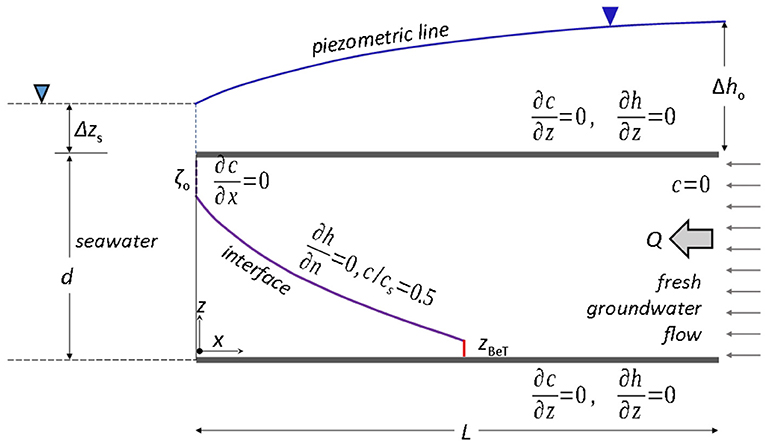
Figure 1. Schematized 2-D confined coastal aquifer, with nominal interface and boundary conditions. Reprinted from Mazi and Koussis (2021).
Upon normalizing the VDF equations by scaling, non-dimensional parameters appear as ratios of characteristic quantities of the SWI-controlling processes. Equations (5–8) present the dimensionless ratios introduced by Mazi and Koussis (2021), in which L [L] is the distance from the shoreline to the aquifer cross-section where the hydraulic head above sea-level is Δh0 [L], d [L] the aquifer thickness, and αL [L] and αT [L], are the dispersivities in the principal directions of transport, i.e., longitudinal and transverse to the flow:
The coupling parameter α compares the regional flow and the convection caused by density differences, or flow resistance vis-á-vis buoyancy, measured by the ratio of the characteristic velocities due to variable density, Kδ, and in its absence, KΔh0/L (Dentz et al., 2006). The Péclet number measures the importance of transport by advection to that by longitudinal dispersion. Mazi and Koussis (2021) showed that the above parameters are related to the dimensionless ratios derived by Henry (1964). Aside from assuming mixing by diffusion instead of dispersion, Di = (|q|/np)αi, the main difference is that Henry took the freshwater flow Q [L−2T−1] as known, as opposed to the hydraulic gradient Δh0/L corresponding to the nominal flow rate Q0 = K(Δh0/L)d. Henry's parameter aH = Q/(Kdδ) and the coupling parameter α are linked via the equation αaH = Q/Q0. The freshwater flow Q depends on α, ξ and the submergence depth Δzs of the aquifer top at the coast (Mazi and Koussis, 2021):
In the unsubmerged case, Δzs = 0, α and aH are related as follows (Dentz et al., 2006):
To date, the VDF equations have only been solved numerically by applying various discretization methods, all demanding considerable effort and CPU-times. The so-called pseudo-coupled VDF equations (Simpson and Clement, 2003) are a compromise in SWI modeling: fluid flow and salt transport are coupled only on the sea-boundary; the salinity distribution is calculated inside the aquifer by neglecting the impact of salinity on the density. However, pseudo-coupled solutions hold only for weak coupling, α ≤ 1 (Simpson and Clement, 2003; Dentz et al., 2006), while under typical field conditions α is on the order of 10 or higher (Mazi and Koussis, 2021).
To bypass this limitation and improve the solution efficiency beyond that of pseudo-coupling, Mazi and Koussis (2021) (1) replaced the seaside boundary by the interface that approximates the streamline separating the through-flow region from the circulating saltwater flow below it, which was taken as stagnant, and (2) prescribed c = 0.5cs on the interface, from where dissolved salt transverse-disperses into the through-flow zone, while at the outflow gap brackish groundwater exits to the sea by advection, ∂c/∂x|x = 0 = 0. With the salinity in the through-flow zone c ≤ 0.5cs, the density contrast δ is halved, as is the coupling parameter α. This enlarges the application range of an SWI model that considers flow and transport as entirely decoupled in the through-flow region, bypassing the high-salinity region near the seaside boundary.
In the present study, we define the through-flow zone and compute the flow field using the analytical solution of Glover (1959). Then, we calculate the mixing of salt along streamlines and their normals, the principal directions (PD) of transport, with the highly efficient 2D-MADPD tracer transport code of Syriopoulou and Koussis (1991) (see Appendix A). The 2D-MADPD model employs the matched artificial dispersivity (MAD) method to resolve the dilemma of numerical diffusion/dispersion vs efficiency in advection-dominated transport. 2D-MADPD is very fast not only because it solves a linear differential equation (hence avoiding the need for iterations to converge at each time step) but also because of employing the principal directions for discretization, which allows to split locally the 2D problem in two 1-D equations. Fast execution of an algorithm is critical when repeated runs are required, as e.g., in Monte Carlo (MC) simulations to handle uncertainties. Uncertainty in this work concerns the hydraulic conductivity and the natural and human-induced stresses of the aquifer. We embed the uncoupled “analytical flow and MADPD tracer transport” SWI model in a stochastic MC modeling framework and estimate the salinity field in the through-flow zone, with uncertainty limits.
The application of the 2D-MADPD model (Appendix A) requires prior definition of the flow net as grid for calculating the transport. The concentrations are computed at the intersections of equipotentials and streamlines. In this study the flow net is determined from Glover's (1959) solution for a confined coastal aquifer of infinite depth; its implementation in a finite-depth aquifer is given in Appendix B. The flow net extends landward to the location where the separation streamline reaches the aquifer base. Glover provides also the specific discharges along streamlines (parameters of the 2D-MADPD model). Regarding the transport boundary conditions, c = 0.5cs is assumed on the separation streamline and zero-flux through the aquifer top, ∂c/∂z = 0. The inflow concentration is zero (freshwater), while no concentration is specified at the outflow section (advection, ∂c/∂x = 0). The solution is algorithmically efficient and straightforward. It is implemented in two stages, grid generation with Glover's solution and integration of the advection-dispersion equation with 2D-MADPD. This application to simulate SWI in the through-flow region of a confined coastal aquifer will be called 2D-MADPD-SWI.
As already mentioned, Glover's solution holds for confined aquifers of infinite depth that real-world aquifers evidently are not. When Glover's solution is applied to a finite-depth aquifer, the separation streamline (interface) crosses the bed at an angle (a streamline coincides with a no-flow boundary). However, we do not expect this error to be significant. A conflict arising due to ignoring the infinite-depth is the incompatibility of the conditions where the separation streamline reaches the aquifer bed. According to the uncoupled solution approach (Mazi and Koussis, 2021), c = 0.5cs is specified on the separation streamline, whereas the aquifer base is a no-flux boundary. To avoid this singularity, Koussis and Mazi (2018) introduced at the interface toe a blunted edge that bends the interface to terminate vertically on the aquifer bed, consistent with the no-flux condition ∂c/∂z = 0, also reducing the interface length. This correction affects the concentrations, not the flow net. However, we use the blunted edge to improve the estimation of the position of the interface toe.
The MAD scheme, though unconditionally stable, can suffer from spurious oscillations. These can be suppressed via grid constraints in terms of the Courant number and the weighting factor θ (Appendix A). As is proportional to the specific discharge, it increases rapidly as the streamlines converge toward the outflow and the grid constraints may not be satisfied in the entire through-flow region. Thus, spurious oscillations cannot be eliminated, but can be constrained. Because the MAD scheme derives from an advection equation, it cannot transmit perturbations upstream. For this reason, and since spurious oscillations at a node can affect only its seaward nodes, it is preferable to adjust the grid density and time step to satisfy the Courant number constraints at the nodes closer to the inflow section. This helps to contain the spurious oscillations in the region near the exit to the sea.
2D-MADPD-SWI was tested generically in four hypothetical confined aquifers, with coupling parameters α = 5, 10, 25, and 50. These α-values correspond to a constant hydraulic head (datum at sea level h0 = Δh0) at the inflow section h0 = 5, 2.5, 1, and 0.5 m, respectively. The Péclet number was in all cases, corresponding to field-relevant dispersive mixing; the aspect ratio was ξ = 0.01 (common in real-world SWI applications), and the dispersivities ratio was rd = 0.1. SWI into the hypothetical aquifers was simulated with FEFLOW (Diersch, 2006a,b) using the coupled VDF equations, to obtain the reference solutions. Steady-state hydraulic conditions were assumed, without hydraulic stress (no pumping). All aquifers were assumed to be homogeneous and isotropic, with hydraulic conductivity K = 103.68 m/d. The sea salinity was assumed to be equal to 35,000ppm TDS and δ = 1/40.
In this study, we employ MC simulations to assess the aquifer response due to uncertainty in the hydraulic conductivity and hydraulic head at the inflow section. To this end, 20 values of the hydraulic conductivity and 20 values of the hydraulic head were generated with a random number generator. A customized random number generator following the triangular distribution (Rozos et al., 2020) was used to avoid the clustering of values. Representative values were obtained over the whole feasible range with a density resembling the assumed (triangular) distribution, even with a limited number of generated values. The triangular distribution has three parameters corresponding to the lowest and highest values of a parameter and to the most probable one (Sprow, 1967). The parameters of the triangular distribution for the hydraulic conductivity were equal to the 50, 150, and 100% of the conductivity of the aquifers. Similarly, the parameters of the triangular distribution for the hydraulic head were equal to the 50, 150, and 100% of the hydraulic head of the aquifer with α = 10.
The Cartesian product of the 20 hydraulic conductivity random values times the 20 hydraulic head random values gives 400 pairs of values. With these pairs of values the 2D-MADPD-SWI model produced 400 solutions, from which 400 salinity lines of 1,500 ppm TDS were obtained. This salinity value was selected because it is the suitability limit for irrigation. These 400 salinity lines were sorted according to the mean value of their x-coordinates, their “x-center.” Then, the lines of which the x-centers correspond to the 5 and 95% percentiles of the 400 x-centers were used to define the 90% confidence interval of the 1,500 ppm TDS line.
The 2D-MADPD-SWI was implemented in MATLAB language and was run in Octave with the parallel package (Watterson, 2021) to allow a parallel execution of the MC simulations.
The Figures 2–5 display the equal-salinity lines simulated with FEFLOW and 2D-MADPD-SWI for the aquifer with α= 5, 10, 25, and 50. The corresponding blunted edge correction lengths are 0.75, 1.84, 6.41, and 18.49 m.
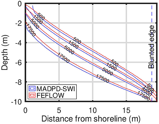
Figure 2. Lines of constant salinity [ppm TDS] of the FEFLOW and 2D-MADPD-SWI solutions for α = 5.
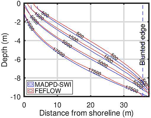
Figure 3. Lines of constant salinity [ppm TDS] of the FEFLOW and 2D-MADPD-SWI solutions for α = 10.
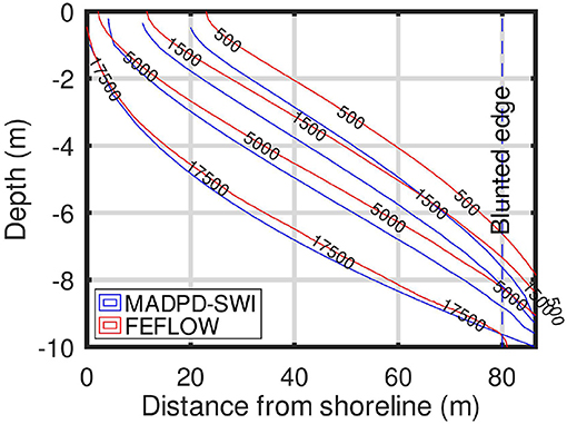
Figure 4. Lines of constant salinity [ppm TDS] of the FEFLOW and 2D-MADPD-SWI solutions for α = 25.
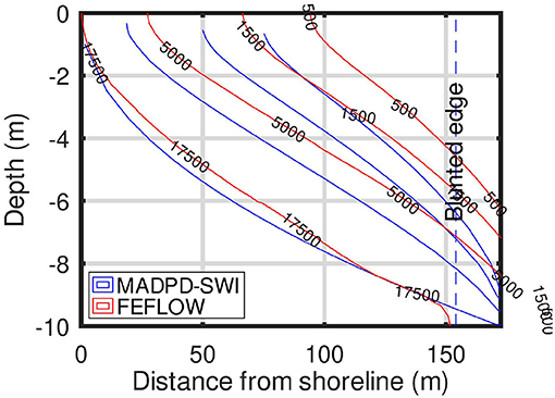
Figure 5. Lines of constant salinity [ppm TDS] of the FEFLOW and 2D-MADPD-SWI solutions for α = 50.
Figure 6 displays the confidence interval of the 1500 ppm TDS line obtained from the MC simulations of the aquifer with α = 10. The realization of a 1,500 ppm TDS line seaward of lines 5 and 95 of this figure has a probability of 5 and 95%, respectively.
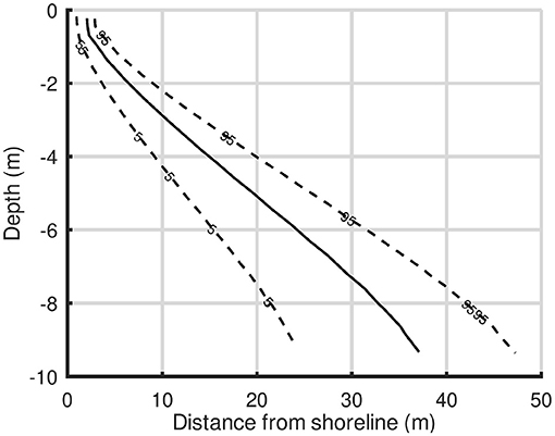
Figure 6. Confidence interval (90%) of the 1,500 ppm TDS line for the aquifer with α = 10.
In the computational complexity theory, there is a category of problems, the nondeterministic polynomial-time complete ones, that is notoriously difficult to solve (Garey and Johnson, 1979). The accurate solution to these problems requires exponential running times; therefore, it is of no practical use. For this reason, for this kind of problem, the heuristic approach is to substitute for the accurate solution a “good solution.” That is a solution that provides an “acceptable accuracy” in a reasonable computational time. A solution is deemed of “acceptable accuracy” if the worst-case performance ratio (PR) is between 2/3 and 4/3 (Balakrishnan et al., 1994). PR is the ratio of the value of a metric obtained for the solution of the heuristic substitute method to the value obtained for the accurate solution. The definition of this metric depends on what characteristics of the solution are considered important.
The method applied in this study can be considered as heuristic, because it does not use the full VDF governing equations. To evaluate its performance, we have defined two metrics that can be considered as the important geometrical characteristics of the mixing zone: (1) the position of the SWI interface toe, and (2) the ratio of the position of the interface toe to the horizontal width of the mixing zone. The worst performance of 2D-MADPD-SWI is observed in the aquifer with α = 50. In that case, the values of the two metrics for FEFLOW are 150 m and 120/150, respectively, whereas the corresponding values of the metrics for 2D-MADPD-SWI are 173 m and 90/173. The corresponding worst-case PR for these two metrics is 173/150, which is well within the [2/3, 4/3] range, and (90/173)/(120/150), which is slightly lower than the lower limit (2/3). Therefore, from a heuristic analysis perspective, 2D-MADPD-SWI may be considered a “good solution.” It should be noted that the value α = 50 is 5 times larger than the common aquifer value, α = 10, reported by Mazi and Koussis (2021).
As mentioned previously, Glover's solution, employed to obtain the groundwater flow net, assumes a confined aquifer of infinite depth. However, the aquifer of the case study has an aspect ratio ξ = 0.01, not an infinite depth. An estimation of the error due to this difference (the overall error is discussed in the previous paragraph) is obtained by comparing the solution of Mazi and Koussis (2021) (their Figure 5) with the solution of 2D-MADPD-SWI (Figure 5). This comparison makes evident that the error due to this is not significant. In fact, 2D-MADPD-SWI provides a better estimation of the mixing zone close to the interface toe compared to the estimation of the uncoupled solution of Mazi and Koussis (2021).
Regarding the CPU times, Mazi and Koussis (2021) mention that the uncoupled solution took 1s under steady-state flow on a PC with an Intel Core 2 CPU 6,300 at 1.86 GHz, whereas the solution of the coupled VDF equations took 193s. The time required to complete 400 runs of the 2D-MADPD-SWI on a PC with a 2-cores AMD EPYC Processor (with IBPB) at 2.5 GHz was 70 s. Therefore, 2D-MADPD-SWI appears to be 5 times faster than the uncoupled solution of Mazi and Koussis (2021). It should be noted that the time reported for 2D-MADPD-SWI includes also the evaluation of the Glover solution to obtain the flow net (which is also the discretization grid of the 2D-MADPD-SWI), whereas the time reported for the uncoupled solution does not include the times required to calculate the SWI interface and to generate the grid. All these render the 2D-MADPD-SWI solution suitable for applications that require multiple runs.
To demonstrate the influence of the uncertainty of the hydraulic properties and conditions on the solution, 2D-MADPD-SWI was embedded in MC simulations. It is noted that a simple simulation with the two most extreme pairs of values (e.g., most favorable and most unfavorable in terms of SWI) would not estimate the likelihood of these extreme values. In contrast, MC can offer vital information in decisions regarding the management of coastal aquifers. For example, the results of the MC simulation shown in Figure 6 can be used to decide on the siting of an irrigation pumping well. If the bottom of that well is placed to the right of the 95% line, then, most likely, the pumped water will be suitable for irrigation (assuming steady conditions). In contrast, placing the borehole inside the confidence interval region increases the risk of withdrawing water of degraded quality. For example, Figure 7 displays a borehole located 30m up-gradient of the toe of the 1,500 ppm TDS line, but within the 90% confidence interval of a hypothetical aquifer that has the same dimensionless ratios as the aquifer of Figure 6 (therefore identical hydraulic behavior). According to the deterministic approach, the water abstracted from that borehole is guaranteed to be suitable for irrigation. However, according to the probabilistic approach, with the MC simulations, there is (roughly) a 30% chance that at some point this borehole will yield water of salinity >1,500 ppm TDS, which is unsuitable for irrigation (Masters, 1991).
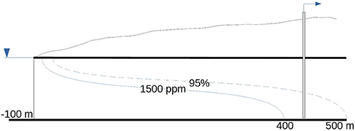
Figure 7. This borehole has roughly 30%chance of yielding water of unsuitable quality within the 90% confidence interval of the 1,500 ppm TDS line.
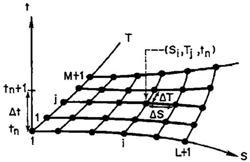
Figure 8. Principal directions co-ordinates and space-time computational grid. Reprinted from Syriopoulou and Koussis (1991).
It should be noted that a careful estimation of the parameter values of the distributions is important. For example, the values of the triangular distribution parameters regarding the hydraulic conductivity should take into account the possible variations dictated by the hydrogeological reconnaissance. The parameter values regarding the hydraulic stress should reflect the short- and long-term hydrologic fluctuations. Ideally, the latter would require a hydrological model to allow the propagation of the uncertainty of the main driver, the precipitation, to the aquifer stresses. In any case, the use of MC simulations to obtain confidence intervals suffers much less from subjectivity compared to any naive interval definition with only two runs, one for the lowest and one for the highest parameter value.
MADPD-SWI can be applied to any type of aquifer. However, Glover's solution can be applied only in homogeneous, isotropic, and confined aquifers of infinite depth to obtain the flow net. Van der Veer's solution can be used in case of unconfined, homogeneous, isotropic, and infinite-depth aquifers. A numerical method could be used to obtain the flow net in the case of an arbitrary aquifer, though in this case the computational complexity would increase, but still remain low compared to a complete VDF model.
In this study we have presented an efficient method for simulating SWI with mixing. This method has been motivated by the need for fast execution to facilitate carrying out multiple runs in Monte Carlo simulations or for identifying optimal management strategies. The method is based on two concepts. The first concept relates to the use of uncoupled SWI equations in the through-flow region of the aquifer (Mazi and Koussis, 2021), instead of the coupled VDF equations in the whole flow domain, combined with analytical calculation of the flow via the solution of Glover (1959). The second concept concerns the use of the principal directions of transport as coordinates on which the computational grid is also defined and as basis for directional splitting of the transport calculations, and the use of the matched artificial dispersivity method (Syriopoulou and Koussis, 1991) to efficiently simulate the longitudinal advection-dispersion processes. Embedding these concepts in the 2D-MADPD-SWI model enabled an at least hundred-fold faster solution than the VDF model. 2D-MADPD-SWI was tested on hypothetical aquifers, the characteristics of which were selected to represent a wide range of real-world situations. The results of the 2D-MADPD-SWI model are comparable to the ones obtained from solving the uncoupled equations with the FEFLOW model. The results of those applications indicate that the worst-case performance of 2D-MADPD-SWI is within what is considered as “acceptable accuracy” in terms of heuristic analysis (Garey and Johnson, 1979).
The CPU time required for a single 2D-MADPD-SWI run on a common modern-day PC was 0.2 s, whereas the time required with FEFLOW for the uncoupled solution was reported to be 1s and for the VDF solution 193 s. The 2D-MADPD-SWI time also includes the automatic generation of the discretization grid along the principal directions of transport. This feature is important, since the grid generation for the finite element method is a demanding process requiring proper care for accuracy and stability.
The low CPU times of 2D-MADPD-SWI allow realizing applications demanding multiple runs. Monte Carlo simulations were applied in one of the hypothetical aquifers to derive the confidence intervals of the 1,500 ppm TDS line (maximum tolerable salinity for irrigation). That example demonstrated the impact of the uncertainty of the hydraulic conductivity and the freshwater flow rate on the advance of the 1,500 ppm TDS line. The management of the coastal aquifers via stochastic simulations is important for two reasons: (1) it provides the means to treat the inherent uncertainty of the properties and conditions controlling the natural processes, and (2) the scientists conducting the study can communicate this inherent uncertainty quantitatively to the responsible decision-making authorities.
Publicly available datasets were analyzed in this study. This data can be found at: https://sites.google.com/view/hydronoa/home/software.
AK: conceptualization. ER: model development. ER and AK: manuscript writing. KM: simulations. All authors contributed to the article and approved the submitted version.
This work has been supported by the Action titled National Network on Climate Change and its Impacts (CLIMPACT) which is implemented under the sub-project 3 of the project Infrastructure of national research networks in the fields of Precision Medicine, Quantum Technology and Climate Change, funded by the Public Investment Program of Greece, General Secretary of Research and Technology/Ministry of Development and Investments.
The authors declare that the research was conducted in the absence of any commercial or financial relationships that could be construed as a potential conflict of interest.
All claims expressed in this article are solely those of the authors and do not necessarily represent those of their affiliated organizations, or those of the publisher, the editors and the reviewers. Any product that may be evaluated in this article, or claim that may be made by its manufacturer, is not guaranteed or endorsed by the publisher.
BOD, biochemical oxygen demand; MAD, matched artificial dispersivity; PD, principal directions; PR, performance ratio; SIF, sharp-interface flow; SWI, seawater intrusion; TDS, total dissolved solids; VDF, variable-density flow.
Aquastat (2016). Water Withdrawal by Sector, Around 2006. Aquastat. Available online at: http://www.fao.org/nr/Water/aquastat/tables/WorldData-Withdrawal_eng.pdf
Bakker, M. (2014). Exact versus Dupuit interface flow in anisotropic coastal aquifers. Water Resour. Res. 50, 7973–7983. doi: 10.1002/2014WR016096
Balakrishnan, A., Magnanti, T. L., and Mirchandani, P. (1994). Modeling and heuristic worst-case performance analysis of the two-level network design problem. Manage. Sci. 40, 846–867. doi: 10.1287/mnsc.40.7.846
Bowen, J. D., Koussis, A. D., and Zimmer, D. T. (1989). Storm drain design: diffusive flood routing for PCs. J. Hydraul. Eng. 115, 1135–1150. doi: 10.1061/(ASCE)0733-9429(1989)115:8(1135)
Christelis, V., and Mantoglou, A. (2016). Coastal aquifer management based on the joint use of density-dependent and sharp interface models. Water Resour. Manage. 30, 861–876. doi: 10.1007/s11269-015-1195-4
Cunge, J. (1969). On the subject of a flood propagation computation method (Muskingum method). J. Hydraul. Res. 7, 205–230. doi: 10.1080/00221686909500264
Custodio, E. (2010). Coastal aquifers of Europe: an overview. Hydrogeol. J. 18, 269–280. doi: 10.1007/s10040-009-0496-1
Dentz, M., Tartakovsky, D., Abarca, E., Guadagnini, A., Sánchez-Vila, X., and Carrera, J. (2006). Variable-density flow in porous media. J. Fluid Mech. 561:209. doi: 10.1017/S0022112006000668
Diersch, H. (2006a). FEFLOW Finite Element Subsurface Flow and Transport Simulation System Reference Manual. Berlin: WASY GmbH Institute for Water Resources Planning and Systems Research.
Diersch, H. (2006b). FEFLOW Finite Element Subsurface Flow and Transport Simulation System User's Manual. Berlin: WASY GmbH Institute for Water Resources Planning and Systems Research.
Diersch, H., and Kolditz, O. (2002). Variable-density flow and transport in porous media: approaches and challenges. Adv. Water Resour. 25, 899–944. doi: 10.1016/S0309-1708(02)00063-5
Frind, E. O., and Germain, D. (1986). Simulation of contaminant plumes with large dispersive contrast: evaluation of alternating direction Galerkin models. Water Resour. Res. 22, 1857–1873. doi: 10.1029/WR022i013p01857
García-Delgado, R. A., and Koussis, A. D. (1997). Ground-water solute transport with hydrogeochemical reactions. Groundwater 35, 243–249. doi: 10.1111/j.1745-6584.1997.tb00081.x
Garey, M., and Johnson, D. (1979). Computers and Intractability: A Guide to the Theory of NP-Completeness. New York, NY: W.H. Freeman.
Ghyben, W., and Drabbe, J. (1889). Nota in Verband met de Voorgenomen Putboring nabij Amsterdam. The Hague: Koninkl. Inst. Ing. Tijdschr.
Glover, R. E. (1959). The pattern of fresh-water flow in a coastal aquifer. J. Geophys. Res. 64, 457–459. doi: 10.1029/JZ064i004p00457
Henry, H. R. (1959). Salt intrusion into fresh-water aquifers. J. Geophys. Res. 64, 1911–1919. doi: 10.1029/JZ064i011p01911
Henry, H. R. (1964). “Effects of dispersion on salt encroachment in coastal aquifers,” in Sea Water in Coastal Aquifers, eds H. H. Cooper, F. A. Kohout, H. R. Henry, and R. E. Glover (US Geological Survey Water-Supply).
Herzberg, A. (1901). Die Wasserversorgung einiger Nordseebaeder, Muenchen. Z. Gasbeleuch. Wasservers. 44, 815–819, 842–844.
Kinzelbach, W. K. H., and Frind, E. O. (1986). “Accuracy criteria for advection-dispersion models,” in Proceedings, Sixth International Conference on Finite Elements in Water Resources (New York, NY: Springer-Verlag), 489–501.
Kourakos, G., and Mantoglou, A. (2009). Pumping optimization of coastal aquifers based on evolutionary algorithms and surrogate modular neural network models. Adv. Water Resour. 32, 507–521. doi: 10.1016/j.advwatres.2009.01.001
Koussis, A. D. (2009). Assessment and review of the hydraulics of storage flood routing 70 years after the presentation of the Muskingum method. Hydrol. Sci. J. 54, 43–61. doi: 10.1623/hysj.54.1.43
Koussis, A. D., Kokitkar, P., and Mehta, A. (1990). Modeling DO conditions in streams with dispersion. J. Environ. Eng. 116, 601–614. doi: 10.1061/(ASCE)0733-9372(1990)116:3(601)
Koussis, A. D., and Mazi, K. (2018). Corrected interface flow model for seawater intrusion in confined aquifers: relations to the dimensionless parameters of variable-density flow. Hydrogeol. J. 26, 2547–2559. doi: 10.1007/s10040-018-1817-z
Koussis, A. D., Mazi, K., Riou, F., and Destouni, G. (2015). A correction for Dupuit-Forchheimer interface flow models of seawater intrusion in unconfined coastal aquifers. J. Hydrol. 525, 277–285. doi: 10.1016/j.jhydrol.2015.03.047
Koussis, A. D., Pesmajoglou, S., and Syriopoulou, D. (2003). Modelling biodegradation of hydrocarbons in aquifers: when is the use of the instantaneous reaction approximation justified? J. Contam. Hydrol. 60, 287–305. doi: 10.1016/S0169-7722(02)00083-9
Kozeny, J., (ed.). (1953). “Das wasser im boden grundwasserbewegung,” in Hydraulik (Vienna: Springer Verlag), 380–445. doi: 10.1007/978-3-7091-7592-7_10
Masters, G. M. (1991). Introduction to Environmental Engineering and Science. Prentice Hall, NJ: Englewood Clifts.
Mazi, K., and Koussis, A. D. (2021). Beyond pseudo-coupling: Computing seawater intrusion in coastal aquifers with decoupled flow and transport equations. J. Hydrol. 593:125794. doi: 10.1016/j.jhydrol.2020.125794
Pool, M., and Carrera, J. (2011). A correction factor to account for mixing in Ghyben-Herzberg and critical pumping rate approximations of seawater intrusion in coastal aquifers. Water Resour. Res. 47:W05506. doi: 10.1029/2010WR010256
Rozos, E., Dimitriadis, P., Mazi, K., Lykoudis, S., and Koussis, A. (2020). On the uncertainty of the image velocimetry method parameters. Hydrology 7:65. doi: 10.3390/hydrology7030065
Rozos, E., and Koutsoyiannis, D. (2010). Error analysis of a multi-cell groundwater model. J. Hydrol. 392, 22–30. doi: 10.1016/j.jhydrol.2010.07.036
Segol, G. (1994). Classic Groundwater Simulations: Proving and Improving Numerical Models. Prentice Hall, NJ: Englewood Clifts.
Simpson, M., and Clement, T. (2003). Theoretical analysis of the worthiness of Henry and Elder problems as benchmarks of density-dependent groundwater flow models. Adv. Water Resour. 26, 17–31. doi: 10.1016/S0309-1708(02)00085-4
Sprow, F. B. (1967). Evaluation of research expenditures using triangular distribution functions and Monte Carlo methods. Indus. Eng. Chem. 59, 35–38. doi: 10.1021/ie50691a009
Syriopoulou, D., and Koussis, A. (1987). Two-dimensional modeling of advection-dominated solute transport in groundwater. Hydrosoft 1, 63–70.
Syriopoulou, D., and Koussis, A. D. (1991). Two-dimensional modeling of advection-dominated solute transport in groundwater by the matched artificial dispersivity method. Water Resour. Res. 27, 865–872. doi: 10.1029/91WR00312
United Nations (2021). Percentage of Total Population Living in Coastal Areas. United Nations. Available online at: https://www.un.org/esa/sustdev/natlinfo/indicators/methodology_sheets/oceans_seas_coasts/pop_coastal_areas.pdf
Van der Veer, P. (1977). Analytical solution for steady interface flow in a coastal aquifer involving a phreatic surface with precipitation. J. Hydrol. 34, 1–11. doi: 10.1016/0022-1694(77)90058-0
Wada, Y., Van Beek, L. P., Van Kempen, C. M., Reckman, J. W., Vasak, S., and Bierkens, M. F. (2010). Global depletion of groundwater resources. Geophys. Res. Lett. 37:L20402. doi: 10.1029/2010GL044571
Watterson, S. (2021). An Expansion of the Genetic Algorithm Package for Gnu Octave that Supports Parallelisation and Bounds. Available online at: https://github.com/stevenwatterson/GA
Werner, A. D., Bakker, M., Post, V. E., Vandenbohede, A., Lu, C., Ataie-Ashtiani, B., et al. (2013). Seawater intrusion processes, investigation and management: recent advances and future challenges. Adv. Water Resour. 51, 3–26. doi: 10.1016/j.advwatres.2012.03.004
Yanenko, N. (1971). “General definitions,” in The Method of Fractional Steps, ed M. Holt (Berlin: Springer), 117–131. doi: 10.1007/978-3-642-65108-3_9
Principal directions of transport have been proven advantageous for numerical simulation in certain kind of problems. For example Frind and Germain (1986), Kinzelbach and Frind (1986), and Syriopoulou and Koussis (1991) have used principal directions (the cross-sectional flow net) to efficiently simulate tracer transport. Natural coordinates, such as streamlines and their orthogonals, are similarly advantageous in the solutions of groundwater flow problems (Rozos and Koutsoyiannis, 2010).
Tracer transport in steady groundwater flow, without internal sources or sinks, is modeled by the advection-dispersion (A–D) equation on the orthogonal Principal Directions of transport (S, T) (streamlines and equipotentials in isotropic aquifers), Figure A1 (Syriopoulou and Koussis, 1991):
where c is the concentration of a conservative solute, u the linear pore velocity along S, and t time; dispersion coefficients are , with αi the dispersivity in the i-direction (S or T), and the molecular diffusion coefficient. Advantages of the PD formulation are a single advective flux term, (q/np)c = uc, with np the porosity, and only two dispersive-flux terms, −DL∂c/∂S and −DT∂c/∂T (diagonal dispersion tensor). At each time step Δt, Equation (1) is split locally in two 1-D equations (Yanenko, 1971), an A–D equation along streamlines S and a dispersion equation in the direction T transverse to the flow:
Derivatives are approximated as finite differences (FDs) ratios on irregular PD grids. Coincident natural co-ordinates and curvilinear gridlines avoid numerical (i.e., artificial) transverse diffusion “essential if dispersive contrast is high (Frind and Germain, 1986)” and help eliminate spurious reactions in reactive-species transport (Garćıa-Delgado and Koussis, 1997; Koussis et al., 2003). c* is computed by solving Equation (2) with the method of Matched Artificial Dispersion (MAD) (Syriopoulou and Koussis, 1991) for one ΔS along each streamline and becomes initial condition for Equation (3). Equation (3) is discretized in the transverse T-direction by centered FDs, centered- or backward-in-time; the resulting tridiagonal system of equations is solved with the Thomas algorithm. This completes integrating Equation (1) for one Δt over the first strip of elements ΔS, ΔT. Repeating the procedure advances the solution to a user-defined edge of the plume (c ≤ ctolerance) and initializes the field for the next time step. The FORTRAN source code (without the Crank-Nicolson option) is listed in Syriopoulou and Koussis (1987).
The MAD numerics solve the wiggles vs smearing dilemma posed by steep fronts in advection domination on the premise that the advection equation approximates the A–D Equation (2) to first order. The dispersion term is truncated and the remaining advection equation is discretized over a grid cell as follows (Cunge, 1969): , with Δc*/Δt = ((c*)n+1−(c*)n)/Δt; ∂c*/∂S≈0.5[(Δc*/ΔS)n+(Δc*/ΔS)n+1], with Δc*/ΔS = ((c*)i+1−(c*)i)/ΔS; i, n mark discrete space and time and θ is a spatial weighting factor. The resulting explicit scheme is
Expanding the grid functions in Taylor series about (Si, tn) to second order and converting second derivatives to second spatial derivatives via the advection equation yield . The right-hand side is the second-order truncation error with numerical diffusion coefficient DN = (0.5−θ)uΔS. Matching DN = DS, via , models longitudinal dispersion; Equation (4) is unconditionally stable for θ < 0.5 (DN = DS>0) and ensures c*≥0 for and ai≥0, or (Cunge, 1969; Bowen et al., 1989; Koussis, 2009); for pure advection θ = 0.5 and . Variable flow is accommodated by averaging velocities over each ΔS. The MAD scheme can be expanded to account for a solute undergoing first-order decay reaction, e.g., BOD (Koussis et al., 1990).
The grid density is defined by the number of equipotential and streamlines of the flow net, respectively, and must be selected carefully, because it not only influences the resolution of the method, but also the MAD scheme's behavior (Appendix A). The potential on each equipotential line is (2δQx/K)0.5, where x [L] the distance of the equipotential line at the aquifer top from the shoreline and Q the freshwater flow rate per unit shoreline-length. The equipotential lines are equidistant. The streamlines are calculated at equal streamfunction intervals, obtained by dividing the maximum streamfunction value, Q/K, by the number of streamlines. The coordinates of the intersections of the equipotentials and the streamlines (the nodes of the PD grid) are calculated by Glover's complex Equation (1). The specific discharge at the intersections is calculated analytically by Darcy's law and Equation (2) of Glover. Also required is the freshwater flow rate Q. If instead the hydraulic head at the inflow section is provided (the outflow section is at the sea boundary), Q is computed from Equation (9) for Δzs = 0. Finally, the buoyancy factor δ is corrected according to Koussis and Mazi (2018), to account for the effects of transverse dispersion.
Keywords: seawater intrusion, mixing zone, Monte Carlo simulations, fast modeling, principal direction, matched artificial dispersivity
Citation: Rozos E, Mazi K and Koussis AD (2021) Efficient Stochastic Simulation of Seawater Intrusion, With Mixing, in Confined Coastal Aquifers. Front. Water 3:720557. doi: 10.3389/frwa.2021.720557
Received: 04 June 2021; Accepted: 26 July 2021;
Published: 19 August 2021.
Edited by:
Xuejing Wang, Southern University of Science and Technology, ChinaReviewed by:
Rong Mao, The University of Hong Kong, Hong KongCopyright © 2021 Rozos, Mazi and Koussis. This is an open-access article distributed under the terms of the Creative Commons Attribution License (CC BY). The use, distribution or reproduction in other forums is permitted, provided the original author(s) and the copyright owner(s) are credited and that the original publication in this journal is cited, in accordance with accepted academic practice. No use, distribution or reproduction is permitted which does not comply with these terms.
*Correspondence: Evangelos Rozos, ZXJvem9zQG5vYS5ncg==
Disclaimer: All claims expressed in this article are solely those of the authors and do not necessarily represent those of their affiliated organizations, or those of the publisher, the editors and the reviewers. Any product that may be evaluated in this article or claim that may be made by its manufacturer is not guaranteed or endorsed by the publisher.
Research integrity at Frontiers
Learn more about the work of our research integrity team to safeguard the quality of each article we publish.