 Martin J. Jolley
 Andrew J. Russell1
 Matthew T. Perks
- 1School of Geography, Politics and Sociology, Newcastle University, Newcastle upon Tyne, United Kingdom
- 2School of Engineering, Newcastle University, Newcastle upon Tyne, United Kingdom
Large-scale image velocimetry is a novel approach for non-contact remote sensing of flow in rivers. Research within this topic has largely focussed on developing specific aspects of the image velocimetry work-flow, or alternatively, testing specific tools or software using case studies. This has resulted in the development of a multitude of techniques, with varying practice being employed between groups, and authorities. As such, for those new to image velocimetry, it may be hard to decipher which methods are suited for particular challenges. This research collates, synthesises, and presents current understanding related to the application of particle image velocimetry (PIV) and particle tracking velocimetry (PTV) approaches in a fluvial setting. The image velocimetry work-flow is compartmentalised into sub-systems of: capture optimisation, pre-processing, processing, and post-processing. The focus of each section is to provide examples from the wider literature for best practice, or where this is not possible, to provide an overview of the theoretical basis and provide examples to use as precedence and inform decision making. We present literature from a range of sources from across the hydrology and remote sensing literature to suggest circumstances in which specific approaches are best applied. For most sub-systems, there is clear research or precedence indicating how to best perform analysis. However, there are some stages in the process that are not conclusive with one set method and require user intuition or further research. For example, the role of external environmental conditions on the performance of image velocimetry being a key aspect that is currently lacking research. Further understanding in areas that are lacking, such as environmental challenges, is vital if image velocimetry is to be used as a method for the extraction of river flow information across the range of hydro-geomorphic conditions.
1. Introduction
Advances in understanding of hydrological processes and the characterisation of river flows have been driven by development of novel sensing instruments, data acquisition platforms, and new analytical techniques (e.g., Chen et al., 2007; Assem et al., 2017; Mishra et al., 2019). Of the recent advances in sensing river flows, arguably the most pronounced is the widespread adoption of acoustic Doppler current profiler (aDcp) technologies (Kostaschuk et al., 2005). This has led to advances in the ability to reliably collect data over large areas, most importantly, entire water columns (Neill and Hashemi, 2018). Whilst this technology offers some advantages over traditional gauging techniques (e.g., ultrasonic sensors, electromagnetic current meters), they fail to overcome a critical limitation in that they require contact with the water-body, which may not be viable during high-flow conditions or where physical access to the channel is not possible.
In recognition of these challenges, the development of non-contact sensors for velocity measurements (e.g., surface velocity radar), and non-intrusive approaches for acquiring bathymetric data (e.g., bathymetric LiDAR, radar, photogrammetry) is now facilitating the non-contact and autonomous monitoring of fluvial flows (Costa et al., 2006; Flener et al., 2013; Javernick et al., 2014; Alimenti et al., 2020). These methods have been shown to provide data as reliable as conventional methods (Costa et al., 2006; Alimenti et al., 2020), but they may be costly to deploy, therefore limiting their widespread adoption of use. They are also subject to their own operational limitations. For example, surface velocity radar is highly dependent on the surface roughness of the river and may be influenced by environmental noise (Fulton, 2020).
An exciting, alternative approach which may be used to determine fluvial flows (when coupled with bathymetric data), is that of large-scale image velocimetry. Research into large-scale image velocimtery has been increasing year-on-year the past two decades, with more of an increasing emphasis on the application of software suites (Figure 1). This technique shares many principles to that of the lab-based image velocimetry method (Lindken et al., 2009), which was initially developed to conduct hydraulic analysis in controlled, laboratory settings. The fundamental principles of the lab-based approach include the seeding of the flow with neutrally buoyant particles, which are then illuminated with laser light and their movement recorded by camera before the particle displacements are determined using either Particle Tracking Velocimetry (PTV) or Particle Image Velocimetry (PIV) (Willert et al., 1996). Whilst large-scale image velocimetry often utilises these same tracking procedures in uncontrolled outdoor environments, certain elements are changed out of necessity and for optimisation of the outputs. Lab-based image velocimetry has been widely adopted with standardised procedures published (e.g., Gollin et al., 2017; Cerqueira et al., 2018). However, the flexible nature of large-scale image velocimetry has meant that techniques and approaches may vary based on the hydrological setting, environmental conditions, and platform of acquisition; this has ultimately made standardisation a more complex activity (Perks, 2020).
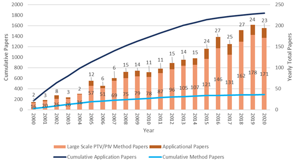
Figure 1. An insight into the number of publications over the past two decades into the research of large scale PIV and PTV, compared with those focused on the application of PIV and PTV on rivers. Data found via www.webofscience.com. The following refinements were applied to the search: Total papers, topic “Surface velocimetry PIV” OR topic “Surface velocimetry PTV” AND all fields “rivers.” Application papers, topic “Surface velocimetry PIV application” OR topic “Surface velocimetry PTV application” AND all fields “Rivers”.
The aim of this review is to present and discuss the key challenges and considerations when seeking to acquire image velocimetry data within a fluvial setting (i.e., large-scale image velocimetry). The key stages in large-scale image velocimetry work-flows can be characterised as (i) capture optimisation (section 2.1); (ii) pre-processing (section 2.2); (iii) image processing (section 2.3); and (iv) post-processing steps (section 2.4), as outlined in Figure 2. Capture optimisation steps involve the appropriate selection of, and preparation of, equipment and its parameters for reliable image sequence capture (e.g., maximising tracer visibility, minimising environmental noise, and ensuring optimal ground sampling distance). Pre-processing steps may be described as those which ensure stable footage with a common spatial reference, with image properties being altered to minimise noise (e.g., removal of visible river bed), and to maximise the signal (e.g., visibility of surface tracers). Processing involves the application of 1D or 2D analysis of feature displacements across a defined field of view. Post-processing steps seek to validate the generated data and remove spurious results. The filtered dataset may then be used to generate secondary products (e.g., discharge) when combined with surrogate information (e.g., cross-section measurements).
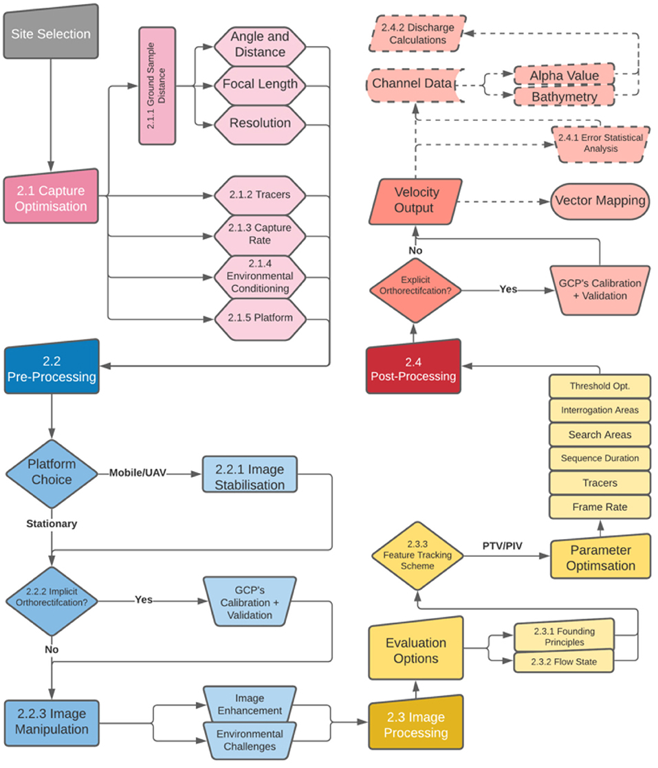
Figure 2. A generalised system of the required processes for analysing river flow using image velocimetry methods. Pink sections are the steps required for capture optimisation (section 2.1), blue represents pre-processing stages (section 2.2), yellow the processing stages (section 2.3), and red shows post-processing stages (section 2.4) (Harpold et al., 2006; Koutalakis et al., 2019; Perks, 2020).
2. Image Velocimetry Processes
2.1. Capture Optimisation
2.1.1. Ground Sampling Distance
The ground sampling distance (GSD) of imagery is the distance between the centroid of two adjacent pixels (Figure 3). The GSD of the imagery used in large-scale image velocimetry analysis is a critical consideration with features smaller than the GSD being poorly resolved. For example, imagery with a GSD of 1 cm/px may include features of 0.008 m length, but these would not be depicted as being any less than 0.01 m length in the imagery. Critically, if the GSD is significantly larger that the individual features present on the water surface, these features may not be visible in the imagery, and these features would therefore be unsuitable for image velocimetry purposes. Although there is no clear guidance on specific values relating to the point at which tracers are no longer visible, generally, a tracer would have to be significantly brighter than the background to dominate the overall contrast of the pixel. As a result of these factors, it is important that the image GSD (cm/px) for the proposed image acquisition settings is known in advance. This will ensure that features visible on the free-surface will be adequately resolved by the camera system. In a scenario where the footage is acquired at nadir, this is governed by the focal length (F; mm), sensor width (SW; mm) and image width (IwP; pixels). Using these characteristics of the camera sensor, and user knowledge of the desired GSD, the required height of image acquisition can be calculated (Equation 1; Pix4d, 2019), see Figure 4.
The image sensor is the apparatus in the camera that converts optical imagery into an electric signal using a matrix of small potential wells (pixels) (Edmund Optics, 2021). The size of image sensor relates to the amount of light a camera can capture, and typical security/IP type cameras use a range between 1/4” (6.35 mm) to a 2/3” (16.9 mm) sensor (Caputo, 2010). Without a large enough image sensor, detail is lost due to a lack of capability to add detail through pixel colour/tone, or due to a high signal:noise ratio seen with smaller sensors (Morrow, 2021).
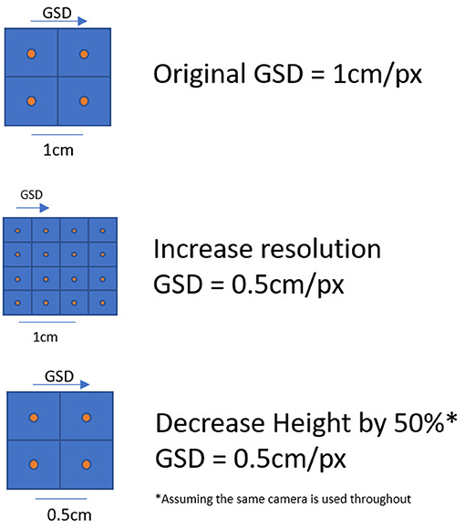
Figure 3. How GSD is described and can be altered using either an increase in resolution, or decreasing the distance between the subject and the camera.
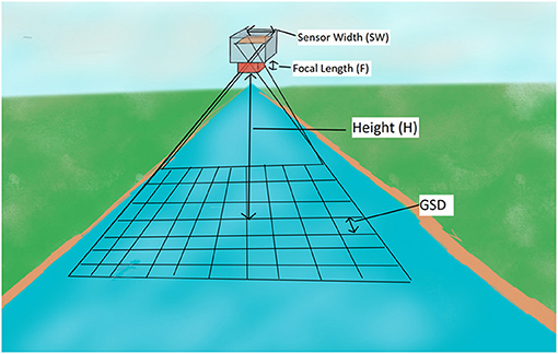
Figure 4. Schematics of GSD of Nadir angle.
Subsequently, the GSD may be affected by the camera angle and the camera distance from the source. Introducing a non-nadir angle to the camera increases the length between the camera and the background of the image, in addition to increasing the width of the coverage. Effectively, with a shift in the pitch of the camera, it will create a trapezoidal shaped image grid, where the background is scaled proportionally to the angle and distance from source. This results in the GSD being variable across the field of view (FOV), and the image background being relatively poorly resolved. For this reason, the sensing of environments using oblique camera angles, particularly over long distances, may result in image acquisition where features on the water surface in the background cannot be easily detected. In instances of oblique image capture, the GSD (cm/px) can be determined using Equation (2), where L is a given length both horizontally (Lh;m) and vertically (Lv;m), IwP is the image width (px) (Equations 3–4), αv is the angle of tilt seen in the roll axis (Equation 3), αh is the angle of tilt seen in the pitch axis (Equation 4). Θ° is the angle of capture (Equation 5), calculated by using the Sensor Width (SW) and the Focal Length (F). These equations are implemented within GSDCalc (Jolley, 2021), Figure 5.
When discussing camera angles, it is important to note the type of camera station in use. Camera stations are typically described as being either fixed or mobile platforms, these are discussed in section 2.1.5. Due to the flexible nature of large-scale image velocimetry, a wide variety of camera angles are adopted. The fixed camera deployments described in Perks et al. (2020) includes camera angles up to 57 degrees from nadir. Alternatively, for mobile cameras, Eltner et al. (2020) suggests that a tilt angle more than 10° from nadir should be avoided where possible. Generally, for both fixed and mobile platforms, the closer that the camera sensor is to nadir the better, providing that the region-of-interest is visible throughout, along with ground control points, and static features to enable stabilisation (when required). Finally, when installing fixed camera stations, a critical consideration is the effect of stage variation of the camera's FOV. As stage increases, the distance between the water surface and camera decreases, which can result in a reduction in the area sensed.

Figure 5. Schematics of GSD at an oblique angle.
Camera focal length (usually given in mm), is the distance between the image sensor and the camera lens when the subject area is in focus. The smaller the focal length, the larger the area captured, but at a smaller apparent size. Subsequently, the larger the focal length, the smaller the area captured, but in higher detail. Generally, cameras have either prime (non-adjustable) or zoom (adjustable) lenses. It has been recommended that independent of the lens used, the internal parameters of the camera should be established (Detert, 2021), and used to removal lens distortion effects prior to the the extrinsic calibration stage (i.e., orthorectification; section 2.2.2).
Finally, the GSD is greatly affected by the image resolution (i.e., number of pixels present within an image). Whilst it may seem intuitive to seek to minimise the GSD by using the highest resolution of imagery available, this approach comes at a time/power cost when undertaking image velocimetry analysis, with the benefits reaching an asymptote once the surface patterns and features in the image can be adequately resolved. This has been demonstrated in lab-based studies. For example, Prasad et al. (1992) observed that when image resolution was reduced by a factor of two, this was accompanied with only a small loss in the ability to detect tracers (equivalent to a loss of 0.3% of “good” features). However, processing speed increased fourfold. Similar findings have also been observed within field settings. Analysis of low resolution imagery (144p, 256 × 144), produced deviations in longitudinal velocity of only 5% relative to full resolution imagery (1,080p) (Le Boursicaud et al., 2016), and negligible changes to velocity results between 1,280 × 720 and 256 × 144 (Leitão et al., 2018). Similarly, Tosi et al. (2020) observed that reducing the resolution of full HD images to 25%, resulted in mean velocity outputs differing by less than 0.05 m/s (<10%), with a reduction in computation time of roughly 23%. Further to this research, it is also demonstrated that reducing the resolution from full (1,430 × 1,080 px) to half (715 × 540 px) reduces power consumption enough to increase the number of cycles that can be performed on a single charge by 30% when using a 5,000 mA/h battery on a single charge (Livoroi et al., 2021). However, a formal analysis and evaluation of the influence of image resolution on resultant accuracy across spatial scales is generally lacking. The lack of consensus regarding the optimal resolution for image acquisition has led to researchers adopting intuition to define appropriate configurations (e.g., Dal Sasso et al., 2018). Ultra-HD and 4K videos could be used to enhance tracer visibility (e.g., when sensing over long distances, or oblique angles), and to enable the sensing of smaller tracers (section 2.1.2). However, the processing power required to analyse higher definition videos is a constraint. In instances where imagery has been acquired at very high resolution (e.g., Ultra-HD and 4K), it may be beneficial to sub-sample the imagery to a lower resolution to improve processing speeds providing tracers are still visible.
2.1.2. Tracers
Tracers are thermally, or optically, distinct features present on the water surface that are advected by the current of the flow. Where hydrological conditions permit (e.g., fast-flowing, turbulent streams), sufficient naturally occurring features (e.g., foam, turbulent structures) may be present for successful image velocimetry analysis (see Figure 6). However, the spatial and temporal distribution of tracers can have a significant bearing on the performance of image velocimetry deployments with Meselhe et al. (2004) recommending that 10–30% of the surface should be traceable throughout the process. More recent work has strongly suggested that the density, dispersion index, and spatial variance of tracers are critical controls on the suitability and performance of image velocimetry approaches (Dal Sasso et al., 2020). Recent research into Seeding Density Indexing (SDI) shows that, by selecting frames to analyse based on optimum tracer characteristics (e.g., dispersion, density), then a reduction in surface velocity error of between 16.1 and 39% can be achieved using either PIV or PTV methods (Pizarro et al., 2020b; Dal Sasso et al., 2021). Consequently, by optimising frame selection based on SDI, discharge errors can be reduced to 0.12–0.4% of the total error seen when not optimising frame selection using PIV methods (Pizarro et al., 2020a). The most recent research into SDI has produced a threshold parameter (τ). τ sets a benchmark for frames and their subsequent SDI values, disregarding data that does not exceed the threshold SDI (Dal Sasso et al., 2021).
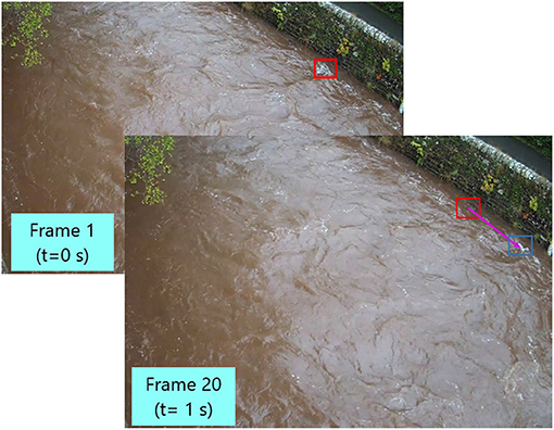
Figure 6. Examples of usable tracers highlighted from a study using a fixed camera with frames exactly 1 s apart.
In instances where the spatial distribution of naturally occurring tracers is sub-optimal, with naturally occurring features that are either inhomogeneous in space and discontinuous in time, artificial tracers may be adopted. This is usually achieved by deploying an environmentally friendly substance such as bark or a decomposing polymer. They should be passive to flow, easily distinguishable, and have no effect on water quality (Detert and Weitbrecht, 2015). The size and the shape of the tracers is also important. As a minimum, tracers should be larger than 1px, which is a function of the ground sampling distance (see section 2.1.1; Dal Sasso et al., 2020), and their size/shape should be stable over time (Tsubaki et al., 2011; Tauro et al., 2017). Wu Tang et al. (2008) experimented with seeding sizes and shapes and determined that for artificially placed tracers, ellipsoidal particles of 2–5 pixels in size perform well. These are not large enough to be greatly affected by internal forces, and are less likely to form agglomerates compared to spherical tracers.
2.1.3. Capture Frame Rates
Commercially available cameras generally have default frame rates that are typically more than sufficient for capturing image sequences required for image velocimetry purposes (i.e., > 5 Hz). Given that the acquisition frame rate is not usually a constraint, the most important aspect is to ensure that the frame rate is consistent throughout the duration of acquisition (Perks, 2020; Detert, 2021), and that it matches the value present within the video metadata. This can be determined through analysis of the time stamps embedded within the on-screen display (Detert, 2021). This is generally configurable to be visible on footage acquired by Internet Protocol (IP) camera systems.
IP cameras are digital cameras which use networked connections to transfer data and can allow the user to access live imagery remotely (Safesite, 2021). Often, these types of cameras are connected to a data logger which can receive, store, and send the imagery. The limitation with some data loggers can be their processing power. For instance, frames can be lost from sequences if using a logger and there is insufficient CPU power. This impacts the time consistency of frames, something that is vital to accurately using image velocimetry.
Complications with these methods can also arise from a lack of bandwidth. Increasing the frame rate has been shown to proportionally increase bandwidth usage (1 fps = 0.179 Mb/s, 10 FPS = 4x more than 1FPS, 30 FPS = 7x more than 1FPS) (IPVM Team, 2021). The relationship between frame rate and bandwidth is not linear due to the way that IP cameras capture frames. IP cameras captures either an I-frame (initial/full frame or a P-frame (predictive frame). I-frames capture the entirety of the FOV and are used as a reference frame, whereas P-frames will only capture changes in an image in relation to the I-frame (Ace, 2013). The report by Ace (2013) also suggests that increasing the I-frame rate from 1 per second does not necessarily greatly improve image quality, but increasing the time between I-frames can significantly reduce image quality.
2.1.4. Managing External Environmental Conditions
The performance of image velocimetry analysis may be influenced by external environmental factors that cannot be easily controlled. These factors include the presence of wind, rain, varied lighting, fog, falling snow, and glare. The impacts of wind are most acutely seen during times of low flow when wind shear may produce a surface expression that is independent of flow velocity (Le Coz et al., 2010). A recent development on the impact of wind demonstrated that, on average, surface velocity deviates by 3% and can reach a maximum of 8%, most typically when wind opposes flow direction and when its magnitude is significant relative to the flow (Peña-haro et al., 2020). The impacts of precipitation are not fully understood but have been reported to blur imagery, ultimately interrupting the processing of data (Fujita et al., 2007). Inhomogeneous lighting and glare on the river surface generates the false impression of colour gradients across the area of interest. This variation in brightness may cause blind spots and the loss of tracer visibility (Hauet et al., 2008; Zhang et al., 2013). Fog impacts velocity results by severely increasing the noise on the surface of the river as it hinders the traceability of surface patterns; acquiring imagery during foggy conditions is generally to be avoided where possible (Zhang et al., 2013). Finally, for falling snow, there is little research in the true impact that it has on velocity results, however, in instances where large scale PIV has been used with falling snow present, authors tend to disregard data due to the scatter that it creates in results (Daigle et al., 2013).
The relative impact that these external environmental conditions have on the quality of image velocimetry results is currently unpredictable, and the overall impacts are currently unknown. Where there are instances of noticeable snow or fog, currently due to the lack of evidence saying otherwise, data should be disregarded. Secondly, the exposure of a monitoring location to variations in wind, precipitation, and glare should be minimised where possible through adjustments in the acquisition methods adopted. For example, in instances with high levels of glare the use of a polarising filter may be beneficial. Alternatively, near infrared (NIR) cameras may act to reduce the severity in brightness difference and may visualise the tracers more prominently. However, it should be noted that application of NIR sensors in some environments may lead to the loss of visible tracers due to attenuation of the NIR signal by the water (Zhang et al., 2013). Whilst future work will seek to provide correction factors for observable external environmental conditions (e.g., wind shear), these relations have yet to be established so their effects should be minimised where possible.
2.1.5. Choice of Platform
Fixed stations allow a specific area of river to be analysed, providing a time-series of images that can be used to determine surface velocities. Usually, fixed stations are commissioned in order to monitor river flows, and to develop and extend discharge rating curves (e.g., Hauet et al., 2008). There are several ways that fixed stations can operate in regards to the capture and processing of data. The study of Tosi et al. (2020) evaluates methods of capturing and processing data in situ to reduce the amount of data that is required to be sent via external networks. This can be useful where stations are in remote locations and affordable networks (e.g., mobile networks), are scarce. Alternatively, as seen in the case studies of Perks (2020), networked cameras (as discussed in section 2.1.3) can be used to stream imagery across a network to be processed either near real-time or at a later date.
Regardless of the proposed fixed station processing method, limitations include the inability to alter the field-of-view without recalculation of the coefficients for converting pixel space to real world distances (see section 2.2.2). Resultantly, there is the potential for the site configurations being optimal under certain flow conditions, but unsuitable during others (e.g., during bypass flows, out-of-bank flows, etc.) Additionally, supplementary information is required in order to properly scale the imagery as a result of fluctuating water levels. This is typically in the form of river stage measurements which enable the distance between the water surface and the camera to be accounted for.
Alternatively, mobile platforms may be used to acquire footage for image velocimetry purposes. An example of this is the use of Uncrewed Aerial Vehicles/Systems (UAVs/UASs), or helicopters in fluvial environments that are hard to reach, dangerous to the operator, or where the inundated extent is greater than the field-of-view of the fixed monitoring station. These approaches have been particularly beneficial for understanding turbulent flows in rivers for sediment transport (e.g., Thumser et al., 2017), capturing flow data at ungauged sites (e.g., Kim et al., 2008), and determining river velocities during periods of high-flow (e.g., Perks et al., 2016). Additionally, this has opened up the possibility of large spatial extents being observed rapidly (e.g., Perks, 2020). Generally, using a mobile platform involves similar processes to those of fixed stations, but requires some extra stages in the pre-processing stage such as image stabilisation (see section 2.2.1). A key advantage of using mobile platforms for image capture over fixed stations is that many of the optimisations listed in section 2.1 could be met (e.g., camera angle being nadir, flexible fields of view, and spatially consistent GSD).
Although UASs are currently the main focus of mobile methods, it is important to note that there are other methods of mobile image velocimetry. Prior to UAS being reasonably attainable, mobile methods could be conducted using telescopic poles, as demonstrated in Le Coz et al. (2010) and Dramais et al. (2011). Secondly, an important revelation of mobile image velocimetry is the use of software on mobile phones (Hain et al., 2016; Caldwell et al., 2019). Lab based studies on the use of mobile discharge apps (e.g., DischargeApp) show that the methods can reproduce discharges without the need of illumination within a 15% error 87% of the time (hand-held), and 100% of the time using a tripod (Carrel et al., 2019).
A more recent and promising advancement is the use of satellite imagery as a capture method, but is still in its infancy of development. There are limitations to using satellite data, such as the limitation of the GSD that is achievable by satellite imagery and whether it is capable of detecting and tracking features on a river surface. For reference on image quality, Kääb et al. (2019) uses satellite imagery to track river-ice and water velocities, and does so with a resolution of 3m using PlanetScope satellite imagery (Planet Labs Inc., 2021), capturing each frame at 90 s intervals. Satellite data stores (such as PlanetScope), are capable supplying high-resolution image sequences (as seen with Kääb et al., 2019), and videos of less than or around 1m resolution (typically nadir). Video footage is usually only captured in the panchromatic band of the central detector and at a frame rate of between 30 and 120 FPS. It is still yet to be seen how well these datasets can provide river flow gauging, and much more research is required into the feasibility of satellites before it can become a recommended method of remote sensing using image velocimetry.
2.2. Pre-processing
2.2.1. Stabilisation
Image stabilisation is required due to the inevitable movement of mobile platforms (e.g., Perks et al., 2016; Bolognesi et al., 2017), and random movements of fixed cameras from vibrations due to influences such as wind or traffic (when fixed on a bridge) (Perks, 2020). Figure 7 demonstrates how images are impacted by stabilisation. Borders of the full initial image are cropped out by the algorithm in each frame (shown as the black boxes around the edges of the image) to only show the sections that are constant (shown in the green overlapping of imagery). Here we can see transformations in both shift and scale due to platform movement. Modern methods of stabilisation may use GPS locations of the camera and/or stable features in the region of interest to create a stable frame of reference for subsequent analysis (Ljubičić et al., 2021).
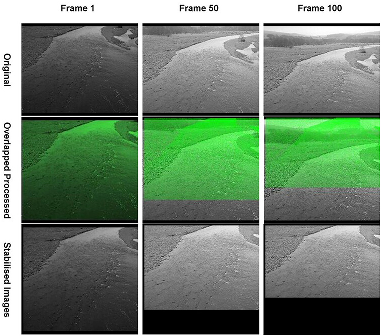
Figure 7. Drone movement shown by overlapping stabilised frames onto original frames. The green mask seen on the processed row highlights where the stable image is within frame, with the final stabilised images cropping all unstable edges.
Stabilisation takes into account the effect of image translation, rotation, and scaling. Translation of the scene is a movement in the image within the xy plane (parallel to the ground). Rotation is a movement that causes a tilt in any direction of the camera (yaw, pitch, and roll). Scaling is impacted by change in platform elevation (z-direction) resulting in changes to the representation of pixel sizes in real world units. When running feature detection algorithms, static points are used and are either detected corner points or clearly distinguishable stationary objects. For a full projective transformation, a minimum of four pairs (eight features), are required (Szeliski, 2006) to match the degrees of freedom (three pairs are required for affine transformations). Stabilised frames are often referenced to either the initial frame, or a subsequently stabilised frame (every nth frame of a series). This may be achieved using a 3D stabilisation technique (e.g., structure-from-motion; SfM), or more commonly a 2D motion estimation technique e.g., single-step discrete Fourier transform algorithm (Guizar-Sicairos et al., 2008), whereby it is assumed that the moving camera is perpendicular to the region of interest and undergoes only changes in the horizontal plane (movements in translation and yaw), and hence, planar transformations are sufficient (Rodriguez-Padilla et al., 2019).
Stabilisation techniques can be manual or automatic. Manual methods rely on a selection of static reference points which are then automatically processed to determine displacement between frames (Rodriguez-Padilla et al., 2019), while automatic methods select features and then track displacements using binary feature matching techniques (e.g., Harris Corner Detection and FAST) (Liu and Cheng, 2008; Muja and Lowe, 2012; Mingkhwan and Khawsuk, 2017). A general process for stabilisation techniques is: breaking down videos into sequential frames, selecting of static features manually or automatically (i.e., feature detection), feature matching and outlier rejection, derivation of transformation function, and image reconstruction and stitching (Tareen and Saleem, 2018). The coordinate grid can either be fixed or be updated throughout the process. Whilst fixed coordinate grids are typically used, the grid may need to be updated over time if there is excessive movement (e.g., translation of the platform). Grids may be altered through the use of similarity, affine, or projective transformations. Accurate transformation depends on the number of point pairs available in the image. Similarity transformations require shifts in the plane parallel to the ground and can result in translational, rotational, and scaling transformations. For these, a minimum of two point pairs are required. Affine transformation includes the same shift changes as similarity with the addition of shear transformations. This requires three point pairs. Finally, for a full projective transformation which includes all of the above as well as perspective deformation, four point pairs are required (Ljubičić et al., 2021).
For fixed cameras, stabilisation is not necessarily required, unless the camera experience movement (e.g., oscillations generated by vibrations, or wind). Detert and Weitbrecht (2015) observed that residual motion of 1 px/s caused by camera shake produced an apparent ground velocity of at least 0.02–0.03 m/s. More recently, Detert (2021) observed that the lack of stabilisation of image sequences acquired using a telescopic pole produced a shift in both image axes by upto ±4 pixels per time step (equivalent to 2 cm in this instance). This unaccounted for movement may substantially impact velocity outputs, especially under flow velocity conditions, relative to the amount of movement seen in frame. When using mobile platforms to acquire footage for image velocimetry purposes, unstabilised image sequences may be a major contributor toward error. An example of this is presented in Detert (2021), where a re-analysis of previously published studies demonstrated that accounting for residual movement reduced errors by 20–30%.
2.2.2. Orthorectification
Following stabilisation of the image sequence (when required), orthorectification needs to be carried out, unless the image is being captured at nadir and image distortion has been removed. This seeks to remove perspective distortion and manipulate the image to represent accurate real-world distances. Orthorectification manipulates an image such that all pixels are of equal real world length, such that when using a camera at an oblique angle, a pixel in the foreground is equivalent to a pixel in the background.
Orthorectification relies on Ground Control Points (GCPs) to calibrate known coordinate points in the field of view (Tauro et al., 2014). GCPs that have known real-world coordinates are established in the frame of view and these are paired with the pixel location of these GCPs. 2D transformations can be made when the GCPs are located on a similar plane to the surface of the river. 2D transformations have an 8-parameter plan-to-plan perspective projection, which requires at least four GCPs at the river free-surface elevation (Fujita et al., 1998; Detert and Weitbrecht, 2015; Detert et al., 2017; Detert, 2021). 3D transformations are made where there are large variations of elevation seen between GCPs and the river surface. If this is the case then the orthorectification matrix will have 11 unknowns and therefore can only be solved with six or more GCPs (Jodeau et al., 2008). It has been suggested that a minimum of 4 GCPs should be used in or immediately around the region of interest to best orthorectify 2D imagery captured orthogonally to the river surface (Detert and Weitbrecht, 2015; Detert et al., 2017; Detert, 2021), however, reliability of orthorectification can only increase with the number of accurate GCPs used. An increase in GCPs used increases the redundancy of the orthorectified system improving the reliability of the results.
The process of orthorectification can either be explicit or implicit i.e., transformations can either be applied to the raw footage (explicit), or to the vector fields (implicit). Higham and Brevis (2019) suggested that orthorectification of the velocity vector field, rather than the imagery, is more effective in most cases, more specifically with PIV examples. The smoothing of data is a process where the extremities of results are normalised and brought closer to the average. When footage undergoes PIV analysis, vectors are created using an average of the interrogation area surrounding it. This process of using the average values for vectors inherently smooths data, reducing the impact that spurious/outlier tracer velocities has on the overall results. If orthorectification is applied after PIV analysis, then any spurious vectors which have been smoothed due to the averaging of the area will have less of an impact on error associated with converting pixel size to real world lengths and consequently velocities. Alternatively, if this is done explicitly, then applying transformations to erroneous velocity values can exaggerate them, reducing accuracy. Conversely, explicit orthorectification has the advantage of ensuring each pixel has the same real-world dimensions prior to processing (Perks, 2020). An example of explicit orthorectification can be seen in Figure 8.
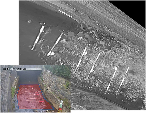
Figure 8. Example of a river surface acquired at Todmorden, UK (bottom left). The red region indicates the region of interest selected by the user. The greyscale image is the orthorectified product produced using KLT-IV.
2.2.3. Image Manipulation
Image manipulation is the process of altering the properties of the acquired images with the aim of reducing interference (e.g., glare, visibility of the river bed, environmental impacts such as wind and rain), and enhancing the visibility of tracers. The first step in the image manipulation process is the conversion of multi-band imagery into single-band imagery (e.g Fujita et al., 2007; Dobson et al., 2014). However, this is not required when footage is captured using a —scale camera (e.g., Patalano et al., 2017), or thermal camera (e.g., Kinzel and Legleiter, 2019). The conversion of multi-band imagery to grey-scale is achieved by eliminating saturation levels and hue, keeping only levels of luminance (Perks, 2020). Subsequent image manipulation is optional but may be beneficial.
Frequently used image enhancement techniques include: intensity normalisation, histogram equalisation, contrast limited histogram equalisation, and binarisation, which are all further explained below (Thielicke and Stamhuis, 2014; The Mathworks Inc., 2020). One of the most important processes for most image velocimetry techniques is to enhance imagery through contrast enhancement steps (Dellenback et al., 2000). Improving the contrast of images helps tracers stand out more in comparison to their environment, making tracking more effective and increasing displacement peak detectability, ultimately improving velocity fields (Deen et al., 2010). Figure 9 highlights the process of typical image processing carried out in PIV and PTV methods. Some of these methods were used in the examples seen in Figure 10.
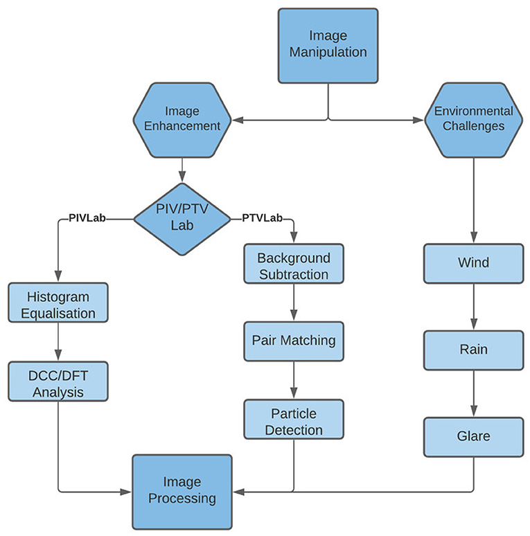
Figure 9. A remodel of the Patalano et al. (2017) study, showing a flowchart for typical image processing sub-sequences with either PIVlab or PTVlab.
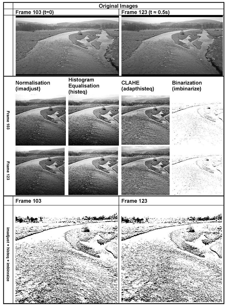
Figure 10. A series of image manipulation processes performed in Matlab using frames from the same video file. Note the amount of information in the binarized images if normalisation and histogram equalisation is performed prior. This shows that there are cases where more than one method of pre processing can improve the amount of data that is traceable by programmes.
Intensity normalisation spreads out the contrast histogram of an image such that a user defined percent of the image is saturated in the high and low intensities. For footage where tracers are barely distinguishable, normalisation may improve the contrast of the colours across the image. Histogram equalisation is the process of enhancing contrast by averaging out the brightness variation across the band. It increases the range and standard deviation of colour histograms and introduces a larger statistical range (Jyoti Bora, 2017). This has been shown to be effective in situations where a colour band shows a cluster of contrast level (Fujita and Aya, 2004). Image binarisation typically uses threshold algorithms to split histograms into two, sometimes using several sub-processes such as background detection and edge detection (Malepati, 2010) to ensure foreground textures stand out as much as possible against their backgrounds (Tensmeyer and Martinez, 2020). This can be especially useful when, despite all previous efforts, tracers are still not prevalent to their background and surroundings. To improve the impact of all image manipulation processes, it would be recommended that footage limits the amount of unnecessary image in frame, and focuses on the area of interest to ensure that the stretch of the normalisation is altering tracers and the water surface, as opposed to surrounding vegetation.
Should the background of the image or river bed be too prevalent in imagery and there is a bias error toward zero displacement, then it is advised that it is removed. To do this, it is possible to use the double-frame background removal process (Honkanen and Nobach, 2005; Patalano et al., 2017). Subsequent frames are analysed and anything that remains stationary between the two frames is defined as background and noise, and therefore can be removed from the image. This will leave only the tracers that have been displaced. Detert and Weitbrecht (2015) makes a point of applying numerous methods of manipulation to achieve the clearest possible tracers. The study uses grey-scaling but also uses a Gaussian filter to remove noise in the background (which helps sharpen edges), then it sets the intensity of pixels below a certain limit to zero and finally performs CLAHE.
To summarise these findings, there is a clear generalisation of processes for image manipulation and pre-processing of videos for image velocimetry. As a minimum, images should be converted to a single-band image (e.g., grey-scaled) and cropped to the area of interest to reduce unnecessary data processing and noise where possible. If tracers are not clearly distinguishable from the surface throughout the video, imagery should be normalised to highlight areas of most intense light and dark, and equalised to further distinguish the average levels of brightness seen across the image. Should this not be enough and the background or bed of the river is still overwhelming the tracking features, Gaussian filters can be applied to decrease image noise and sharpen edges or background removal can be used to remove the background altogether, followed by a binarisation of the image in an attempt to isolate the tracers.
2.3. Image Processing
2.3.1. Founding Principles
The founding principles upon which image velocimetry algorithms are based, stem from either Eulerian or Lagrangian techniques, which are used to describe inter-dimensional flows (Hirt et al., 1974). These techniques are then applied to image velocimetry methodology. Lagrangian is the basis of PTV methods, and Eulerian is the foundation of PIV methods (Amelinckx, 1971; Euler, 2008). These principles alter the way that we perceive and record velocimetry data such that, if we were to record an identical point at the same instant using both methods, similar results are not guaranteed (Durst et al., 1984). With Lagrangian/PTV motion, the particle's velocity vector can be described at any given point in space-time. It provides a complete assessment of the dynamics of a fluid particle, knowing where the particle is in any given moment and what velocity it possess, making it a function of time in respect to an initial position (Price, 2006). Conversely, the Eulerian/PIV approach is the movement of a fluid past a control volume of known coordinates, making the velocity a function of a fixed space and time.
Problems can occur with Lagrangian/PTV motion when using natural tracers, as natural tracers are not entirely stable in structure and are capable of deformation, breaking-up, agglomerating, and interacting with one-another. Deformation of tracers also impacts upon the tracking of a centre of mass which, if a tracer deforms, can change position and ultimately impact the assessment of the tracers dynamics. For Eulerian/PIV, cross-correlation methods are used to determine patterns on the river surface and does allow for some transformations in tracers, so long as the 2D patterns are broadly consistent between the interrogation and search areas (Keane and Adrian, 1992).
2.3.2. Flow State
Steady flow is used to describe fluid properties that remain constant with time, while unsteady flow does not. In the case of open channels where velocity is the property in question, we must look at the rate of change of velocity in respect to time, also known as acceleration. For steady flow, we require that , whereas for unsteady flows . One of the core assumptions of Eulers equation of motion is that of steady flow (Euler, 2008). Eulerian motion and PIV focuses on set of known locations of flow and represents an average of a body of fluid through a known location at a specific time (Durst et al., 1984). Although this average can potentially represent useful analysis of a body of fluid regarding an average of flow velocity for use in discharge estimation, challenges arise when sections experience multi-dimensional acceleration, as a variation of velocity as the steady state assumption is not met. Lagrangian and PTV does not encounter similar issues regarding flow steadiness because its foundations are built around calculating the particles position at any given moment in time (Durst et al., 1984). These conditions are typically assumed as reasonable for many applications of PIV as the technique tends to analyse two consecutive images with only a minor time-step.
2.3.3. Feature Detection and Tracking Schemes
PIV and PTV adopt differing principles for the determination of flow velocities. PIV uses an Eulerian understanding of flow motion, using dimensions of length along the river as search areas, utilising tracers or visible patterns that pass through or along these sections to calculate instantaneous velocity vectors for each area. Conversely, PTV uses the Lagrangian approach to calculate flow velocity, focusing on individual particles of flow visible on the surface and tracking their movement through space.
PIV utilises search and interrogation areas within an image to obtain particle displacements (Figure 11). Small window interrogation areas are tracked within larger search areas, and the centres of the interrogation areas are measured regarding distance and divided by the time between frames to produce an average velocity over that search area (Muste et al., 2008). This approach has been shown to be capable of producing highly accurate results (e.g., Creutin et al., 2003; Muste et al., 2008). Given that a collection of individual tracers (surface patterns) are used to infer displacement, this approach is less sensitive to the transformation of individual features. However, inhomogeneity and discontinuity of tracers are critical issues that may negatively affect the quality of PIV analysis. In these instances, PTV techniques may perform better over PIV techniques (Tauro et al., 2016).
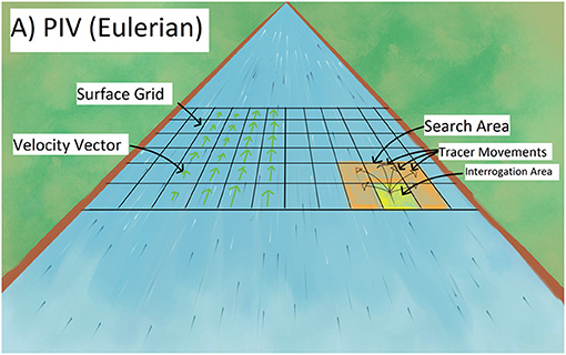
Figure 11. Schematics of general PIV (A) mechanics.
PTV-based approaches (Figure 12), rely on tracking individual particles along a long-profile. This technique has been shown to perform well under low seeding density conditions (Lloyd et al., 1995; Tauro et al., 2017). However, analysis may be adversely affected in instances where tracers change shape, size and from time-to-time disappear from frame. The greater number of tracers that are successfully tracked, the higher the probability of producing an accurate representation of the surface velocity. However, as the number of tracers increases, the required processing time/power also increases. The presence of very high tracer densities may also increase the ambiguity of the individual tracer detection and tracking process (Zhang et al., 1997). There are a range of particle detection and tracking algorithms available for PTV. For feature detection, Good Features to Track (GFTT) (Shi and Tomasi, 1994), FAST (Rosten and Drummond, 2006), and SIFT (Lowe, 1999). For tracking algorithms, cross-correlation can be used, but there are also others such as Kanade-Lucas-Tomasi (KLT) (Tomasi, 1991; Perks, 2020), and variations of the Nearest-Neighbour algorithm (e.g., Tauro et al., 2019).
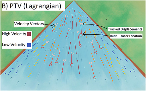
Figure 12. Schematics of general PTV (B) mechanics.
Studies into the optimisation of processing using synthetic models have been highly successful in recent years in highlighting potential areas that are prone to causing errors in velocity results. The importance of the synthetic studies is to aid in selecting appropriate optimisations for differing scenarios (e.g., video length and frame rate). Both Pumo et al. (2021) for LSPIV and Dal Sasso et al. (2018) for PTV methods concur with the Pizarro et al. (2020a) study in that the concentration of particles are a crucial variable in relation to relative error. They also agree that, where seeding density is below-optimal, longer durations of imagery are required and that the contour region around the border of frames should not be included within analysis. These current pieces of synthetic research, however, acknowledge the studies are not exhaustive in variables considered, and more is required to cover more areas of associative error.
Table 1 summarises software suites that are available for users that wish to perform PIV or PTV analysis. Each software will have its own feature detection and tracking scheme, along with varying methods of preparing and presenting data. Each software suite comes with a user-friendly GUI to load in imagery and perform several pieces of analysis on. The suites listed in this table are open-source or freely available to use.
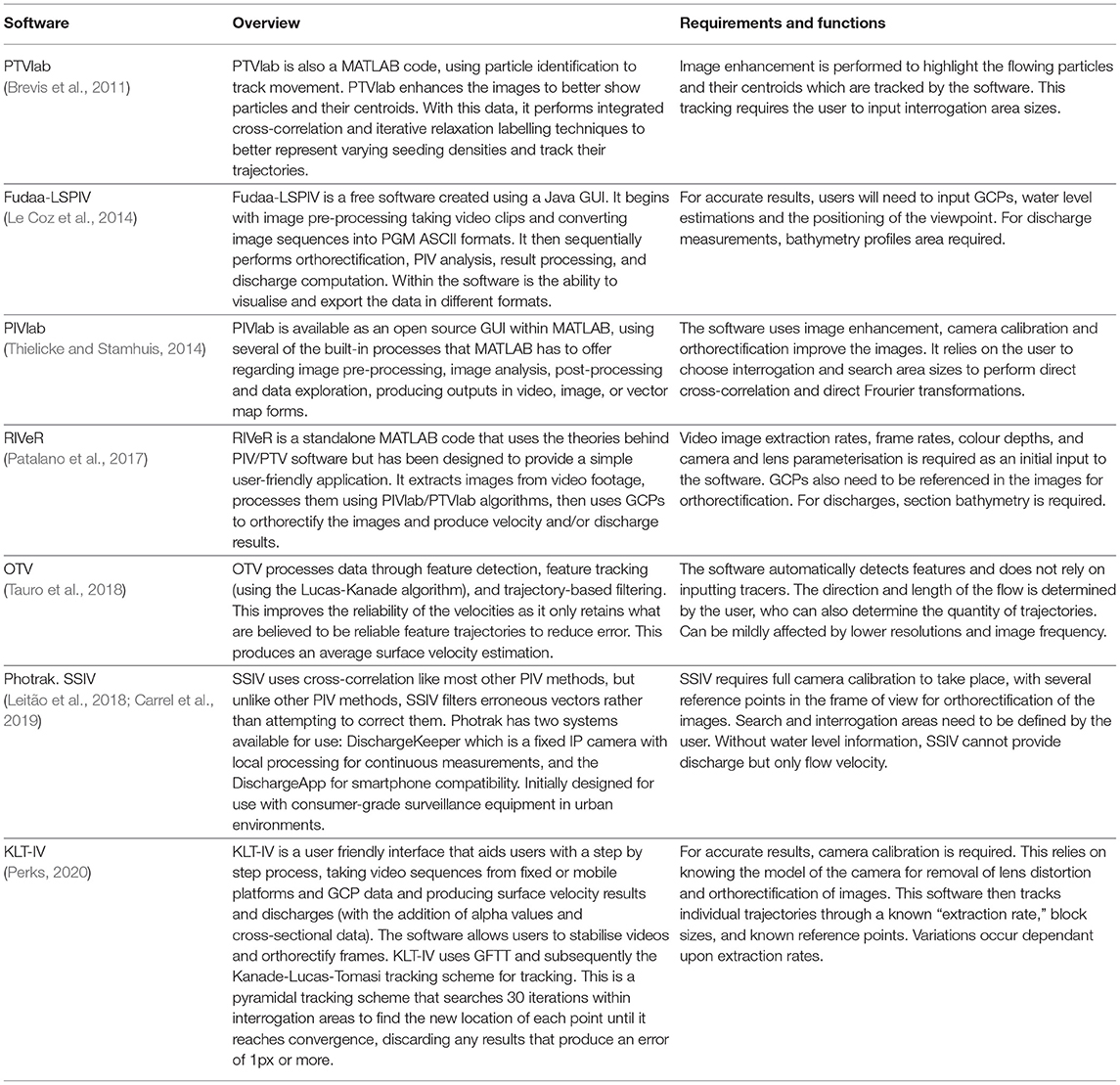
Table 1. A non-exhaustive, generalised, overview of software suites that are currently available with some of their requirements and functions listed.
2.4. Post-processing
Post-processing has two main elements; error reduction (e.g., vector correction, section 2.4.1), and velocimetry application (section 2.4.2). Error reduction is the process of highlighting and filtering possible erroneous datasets and velocity fields, while progressive calculations can use the velocity data and apply it to secondary datasets, such as when using the surface velocities to calculate discharge (through the incorporation of alpha values and bathymetry information).
2.4.1. Vector Correction
Post-processing may reduce errors through the application of statistical methodologies to highlight and filter erroneous outputs. For PIV, details of vector validation can be found in the study of Raffel et al. (2018), which implements several statistical methods of achieving data validation. Statistical validation methods perform similar techniques to distinguish outliers in PIV data, and do so typically by comparing vectors to its surrounding neighbours (Hart, 2000; Masullo and Theunissen, 2016). Alternatively, there is a bootstrapping technique available that does not generate statistics from its nearest neighbours, but instead, a statistic is generated for each component (Pun et al., 2007). Typically, the difference between each method is the type of statistical calculation applied to determine outliers. The basic statistical methods include, but are not limited to, vector difference tests, median tests (Westerweel, 1994), and normalised median tests (Westerweel and Scarano, 2005). Masullo and Theunissen (2016) suggests that overall, the most common detection techniques used in practice are the universal outlier detection scheme (adaptation of median test but normalises the median residual with respect to an estimate of local variation) (Westerweel and Scarano, 2005), and the distance-weighted universal outlier detection scheme for unstructured data (a generalisation of the universal outlier detection method, but with a variance in the definition and weighting to neighbouring vectors) (Duncan et al., 2010). These should be used in all studies where spurious vectors are evident (especially with evident turbulence) (Westerweel, 1994), or results of velocimetry are being used for further applications (e.g., discharge).
Typically, corrective methods for spurious vector will perform statistical analysis as seen above to detect outliers and determine if it falls under a set threshold as to whether or not it is likely a false reading or likely to be reliable. If it is determined to be erroneous, the vector should be removed and replaced using most commonly, a 2D interpolation, or alternatively linear or polynomial interpolation (Stamhuis, 2006). Some common PIV statistical corrective methods are: Penalised Least-Squares Method (Tang et al., 2017), Kriging Regression (De Baar et al., 2014), and Proper Orthogonal Decomposition Outlier Detection (POD-OC) (Wang et al., 2015). Replacing these vectors is important to ensure the results produce statistically meaningful velocities, and without it, can limit the accuracy, resolution, and usefulness of PIV (Hart, 2000).
For PTV data, detecting erroneous vectors is slightly more challenging due to its unstructured features (i.e., does not conform to a gridded system when processing, like seen with PIV methods). Many common PTV algorithms stem from techniques used by PIV regarding the way that it associates vectors with its nearest neighbours, but are altered to deal with the issue of identifying neighbouring vectors in PTV, and not being equally spaced. For PTV validation and correction, should there be more than 15% of outliers, automated programmes could potentially fail to highlight them due to algorithms using neighbouring velocities to determine what classifies as an outlier and should there be a high percentage of outliers, determining what is correct, and what is not, is challenging (Duncan et al., 2010).
Techniques for PTV error correction typically involve a smoothing of displacement fields to use as a baseline to outliers (e.g., Akhmetbekov et al., 1996; Young et al., 2004). Duncan et al. (2010) constructed the Universal Outlier Detection Scheme (which can be used for both PIV and PTV), but it is a development of the algorithm from the Westerweel and Scarano (2005) study for PIV correctional algorithms. An alternative to these methods, is a model based technique (e.g., Young et al., 2004), which has been shown to validate upto 25% of outliers. In this study, the model is described as a 5-stage process. The first stage is initialisation, which involves displacement normalisation, the building of constraints, and then a regularised version of the displacement field is calculated. Secondly is relaxation, this stage produces a displacement field where invalid estimates are replaced with statistically more likely vectors. Third is point removal which uses several statistical methods to determine validation scores (based on user defined thresholds and a T value determined in the relaxation stage). The next stage is attraction designed to iterate landmarks toward their associated termination landmarks. Finally, displacement interpolation which can be used to estimate the displacement at any position in the image field.
2.4.2. Velocimetry Applications
The most common application for image velocimetry datasets is attempting to calculate discharge. Discharge can be calculated with the introduction of known, measured, transects of the river within the camera field of view. These transects can be part of the geo-referencing local coordinate system and measured at the same time as the GCPs. For the discharge calculations to be as accurate as possible, when using PTV methods especially, the river surface needs to have a good spread of tracers, and where this is not the case, it is possible to interpolate or extrapolate measurements using polynomial, cubic, or the constant Froude method (Perks, 2020). Typically, discharge can be estimated using a velocity-area method, introducing typical fluid mechanics parameters [e.g., depth-average velocities, influenced by α (Le Coz et al., 2010)]. When calculating α values, vertical velocity profiles can be found using an aDcp, but Creutin et al. (2003) finds that using 0.85 is a reasonable assumption where this is not possible. Combining α with the calculated velocity, along with bathymetry can give reasonable discharge calculations as found with many studies on river discharge (e.g., Kim et al., 2008; Le Coz et al., 2010; Perks, 2020).
An issue to consider when studying river discharge via velocimetry is the variation of river channel cross-sectional area due to rising stage scour and waning stage fill, or due to passage of sediment waves and bed forms even in more steady flows. It is suggested that after peaks of high flow that river bathymetry is remeasured to ensure that cross-sections are as accurate as possible.
More recently, as an alternative to using estimated alpha values, mobile image velocimetry techniques have been used to derive Gauckler-Manning-Strickler coefficient (K), for cross-sectional roughness in rivers (Bandini et al., 2021). The method simultaneously solves for K and discharge using both linear equations of Manning's and the mean-section method for computing discharge from depth-average vertical velocity. The uncertainty at the 95% confidence level resulted in most of the observations to be near ±10% of the in situ discharge measurements. This method can be used to counter issues with streams that are non-ideal (e.g., highly meandering, non-uniform in slope, etc.).
For users who are looking to apply image velcoimetry to analyse data for the first time, it can be difficult to understand which method (PIV or PTV), to use. The research presented throughout this study should provide some indication on what is the best method for the particular datasets. For further information to help aid decision making regarding methodology choices and how to best apply PIV or PTV, see Table 2. These papers have been studied and briefly summarised regarding the background of the site, the hardware that the method uses, and the results that are discussed by the author. This also includes the challenges that the author faced, as well as the possible causes for such challenges. These papers have been selected as they provide similar but different methodologies using PIV or PTV (e.g., fixed platforms, mobile platforms, thermal cameras).
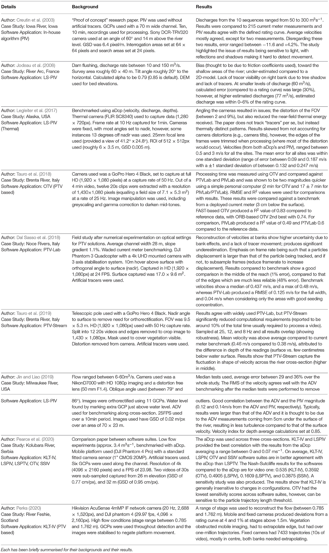
Table 2. A selection of application papers chosen due to their variation of hardware and software suites.
3. Conclusion
Over the last two decades researchers have created numerous techniques for both PIV and PTV methods. Algorithms have been shown to be capable of estimating surface velocity accurately (compared to that of aDcp's), however, the onus is on the user to decipher the ideal methodology. The aim of this research was to present and discuss instances of best practice for image velocimetry processes based on existing papers and case studies, summarised by Figure 2. Where this study has stated it was not viable to suggest an optimal setting due to the lack of information surrounding the topic, example case studies were provided in an attempt to suggest precedence as an alternative.
Research was categorised into four main topics: capture optimisation, pre-processing, processing, and post processing. For capture optimisation, GSD should be as small as possible without having to rely on high resolutions. Adding an angle to the camera can skew GSD in the background of images and this should be accounted for where the region of interest overlaps foregrounds and backgrounds. Tracers are a critical part of image velocimetry techniques and it is important that they remain stable and cover at least 10-30% of the region of interest consistently. It is important that frame rates remain constant throughout the process and this can be checked against time stamps provided by most video cameras. The choice of platform used to capture data depends on the event that is to be captured. For capturing single events or for short term studies, UAS can be used but needs additional steps such as stabilisation. For longer studies such as monitoring river flows and developing discharge rating curves, fixed stations can be used to provide a time-series of images.
For mobile stations, stabilisation is a critical component to the process, sometimes the same is true for fixed cameras that witness oscillations or vibrations due to external influences. For the best results, it is suggested that at least four pairs are used for a full projective transformation to be available and can be selected either manually or automatically. It is also possible to use GPS tracking to detect movement of the camera. The best features to use are static points such as corners of structures. Orthorectification is also required where the camera angle is not nadir. An absolute minimum of six GCPs is required, however, it is the case of the more the better. At least four GCPs should be in the immediate area of the region of interest. If tracers are not prevalent throughout the imagery, it is suggested that imagery is manipulated using contrast enhancement steps. After enhancement, should tracers still not be defined against the background, further image enhancement steps can be applied such as binarisations. As a minimum, images need to be greyscaled and cropped where possible.
Lagrangian and Eulerian algorithms are the basis for PTV and PIV respectively. Each mechanic of motion has its own assumptions and limitations, but also their own advantages. Where tracers are dense and interact with one another consistently or deform and break up, Lagrangian motion is difficult to define. Conversely, for Eulerian, a steady state of flow and tracer availability is required for reliable results. Steadiness of flow is not as much of an issue for Lagrangian techniques as it defines the particles energy and location at any moment of time. PIV methods can be used with more confidence if there are a steady amount of tracers throughout the whole time of processing, providing an output of average velocity across a gridded system on the surface of the river. PTV methods are more detailed, in that they trace an individual particles movement along the longitude of the river surface and can work well where seeding is more scarce.
After calculating surface velocities, general practice should include the detection of outliers and either the removal or the replacement of said outliers. There are numerous statistical algorithms available to the user to aid in achieving corrected velocity vectors, mostly using a statistical means (e.g., median tests), and the nearest neighbouring vector; errors are then replaced using interpolation methods. This is achievable for both PIV and PTV data, however, more research has been done into PIV corrective techniques because of its results being gridded and structured, making the nearest neighbours easier to identify computationally. From this research it is suggested that any datasets being used in further calculations or designs (e.g., discharge), should undergo statistical validations and corrections. Discharge calculations rely on an alpha value being used (typically around 0.85), which estimates the average depth velocity. The alpha value coupled with the bathymetry of a known transect of the river can be used in an area-velocity method of calculating discharge. Where surface velocity is not constant (due to lack of tracers or anything else), velocity can be interpolated or extrapolated using the data readily available from the rest of the river. This can then be used in calculating discharges.
Image velocimetry is a process upon which each stage is ultimately dependant on the previous. Without adequate consideration in prior steps, subsequent stages cannot be relied upon to accurately convey flow data. This research has depicted many of the aspects that require careful planning regarding the best practice for PIV and PTV methods. There are many studies currently available, cited in this research, that allow a user to deduce how to optimally capture and process imagery, either through experimental evidence or through applied precedence. Some stages are less evidenced than others, and require the users intuition to best determine methodology; one of the most important of these, arguably, is GSD. GSD is a complex balance between detail and resources, it is a mix of physical characteristics such as distances and angles, coupled with resolutions and hardware (sensors and lenses). Without optimising GSD to be small enough for a specific site, detail is lost and can hinder the processing capability of PIV/PTV through the lack of ability to detect and track good features. Alternatively, too small of a GSD could critically increase the processing power, storage, and bandwidth requirements to a point that they are unjustifiable. With that being said, it is also vital that stabilisation is competently applied. Stabilisation, where platform movement is detected, can be just as critical as GSD, as research shows that large positional errors can be removed with a good, accurate stabilisation being applied to the imagery. Decisively, however, as previously stated, PIV and PTV are processes with each stage as important as its predecessor and that one of the main limitations with the ideal settings suggested throughout this research, is that it conforms to a generalised process. This means that, despite there being sufficient evidence for the optimal practices suggested, there is always a need for discretion from the user to best meet the requirements for their brief; such as challenging terrains or budget limitations.
To conclude, image velocimetry is a well researched field. The algorithms that are currently available to users tend to prove effective for remote sensing of river surface velocities. As there are currently many software suites available for processing of imagery (e.g., PIVlab, PTVlab, KLT-IV, etc.), a shift of emphasis should be made from focusing on the use of a single algorithm and stating its error bounds, to optimising the methodology of a study to suggest best practice and choice of algorithm and its corresponding variables. With that said, areas such as environmental conditions and the errors associated with them require further study to determine the overall impact that they can have on results, and if possible, quantifying so that further optimisation to the processing system can be suggested, depending on the conditions of time of image capture.
Author Contributions
MJ, MP, and AR contributed to conception and design of the study. This paper was researched and written by MJ. All figures were created by MJ. All authors contributed to editing and reviewing of the manuscript.
Conflict of Interest
The authors declare that the research was conducted in the absence of any commercial or financial relationships that could be construed as a potential conflict of interest.
Publisher's Note
All claims expressed in this article are solely those of the authors and do not necessarily represent those of their affiliated organizations, or those of the publisher, the editors and the reviewers. Any product that may be evaluated in this article, or claim that may be made by its manufacturer, is not guaranteed or endorsed by the publisher.
Acknowledgments
MJ is in receipt of an EPSRC PhD studentship awarded to Newcastle University (EP/R51309X/1).
References
Akhmetbekov, Y. K., Markovich, D. M., and Tokarev, M. P. (1996). A Novel Correction Algorithm for PTV. 3–4. Available online at: http://tokarevmp.narod.ru/site/articles/myarticles/piv07.pdf
Alimenti, F., Bonafoni, S., Gallo, E., Palazzi, V., Vincenti Gatti, R., Mezzanotte, P., et al. (2020). Noncontact measurement of river surface velocity and discharge estimation with a low-cost Doppler Radar sensor. IEEE Trans. Geosci. Remote Sens. 58, 5195–5207. doi: 10.1109/TGRS.2020.2974185
Amelinckx, S. (1971). Classical dynamics of particles and systems. Phys. Bull. 22:157–8. doi: 10.1088/0031-9112/22/3/020
Assem, H., Ghariba, S., Makrai, G., Johnston, P., Gill, L., and Pilla, F. (2017). “Urban water flow and water level prediction based on deep learning,” in Lecture Notes in Computer Science. ed LNCS (Springer), 317–329. doi: 10.1007/978-3-319-71273-4_26
Bandini, F., Lüthi, B., Peña-Haro, S., Borst, C., Liu, J., Karagkiolidou, S., et al. (2021). A Drone-Borne method to jointly estimate discharge and manning's roughness of natural streams. Water Resour. Res. 57. doi: 10.1029/2020WR028266
Bolognesi, M., Farina, G., Alvisi, S., Franchini, M., Pellegrinelli, A., and Russo, P. (2017). Measurement of surface velocity in open channels using a lightweight remotely piloted aircraft system. Geomat Nat Hazards Risk 8, 73–86. doi: 10.1080/19475705.2016.1184717
Brevis, W., Nino, Y., and Jirka, G. H. (2011). Integrating cross-correlation and relaxation algorithms for particle tracking velocimetry. Exp. Fluids. 50, 135–147. doi: 10.1007/s00348-010-0907-z
Caldwell, L., Armijo, D., Mukherjee, S., Minichiello, A., Truscott, T., and Kulyukin, V. (2019). “Work in progress: mobile instructional particle image velocimetry for stem outreach and undergraduate fluid mechanics education,” in ASEE Annual Conference and Exposition, Conference Proceedings (Tampa, Florida).
Caputo, A. C. (2010). “Digital video hardware,” in Digital Video Surveillance and Security, ed Anthony C. Caputo (Elsevier), 39–88. doi: 10.1016/B978-1-85617-747-4.00003-2
Carrel, M., Detert, M., Pena-Haro, S., and Luethi, B. (2019). “Evaluation of the DischargeApp: a smartphone application for discharge measurements,” in HydroSenSoft, International Symposium and Exhibition on Hydro-Environment Sensors and Software (Madrid).
Cerqueira, R. F., Paladino, E. E., Ynumaru, B. K., and Maliska, C. R. (2018). Image processing techniques for the measurement of two-phase bubbly pipe flows using particle image and tracking velocimetry (PIV/PTV). Chem. Eng. Sci. 189, 1–23. doi: 10.1016/j.ces.2018.05.029
Chen, Q., Zhang, Y., and Hallikainen, M. (2007). Water quality monitoring using remote sensing in support of the EU water framework directive (WFD): a case study in the Gulf of Finland. Environ. Monitor. Assess. 124, 157–166. doi: 10.1007/s10661-006-9215-8
Costa, J. E., Cheng, R. T., Haeni, F. P., Melcher, N., Spicer, K. R., Hayes, E., et al. (2006). Use of radars to monitor stream discharge by noncontact methods. Water Resour. Res. 42. doi: 10.1029/2005WR004430
Creutin, J. D., Muste, M., Bradley, A. A., Kim, S. C., and Kruger, A. (2003). River gauging using PIV techniques: a proof of concept experiment on the Iowa River. J. Hydrol. 277, 182–194. doi: 10.1016/S0022-1694(03)00081-7
Daigle, A., Bérubé, F., Bergeron, N., and Matte, P. (2013). A methodology based on particle image velocimetry for river ice velocity measurement. Cold Regions Sci. Technol. 89, 36–47. doi: 10.1016/j.coldregions.2013.01.006
Dal Sasso, S. F., Pizarro, A., and Manfreda, S. (2020). Metrics for the quantification of seeding characteristics to enhance image velocimetry performance in rivers. Remote Sensing. 12. doi: 10.5194/egusphere-egu21-9229
Dal Sasso, S. F., Pizarro, A., Pearce, S., Maddock, I., and Manfreda, S. (2021). Increasing LSPIV performances by exploiting the seeding distribution index at different spatial scales. J. Hydrol. 598. doi: 10.1016/j.jhydrol.2021.126438
Dal Sasso, S. F., Pizarro, A., Samela, C., Mita, L., and Manfreda, S. (2018). Exploring the optimal experimental setup for surface flow velocity measurements using PTV. Environ. Monitor. Assess. 190:460. doi: 10.1007/s10661-018-6848-3
De Baar, J. H., Percin, M., Dwight, R. P., Van Oudheusden, B. W., and Bijl, H. (2014). Kriging regression of PIV data using a local error estimate. Exp. Fluids. 55. doi: 10.1007/s00348-013-1650-z
Deen, N. G., Willems, P., Sint Annaland, M. V., Kuipers, J. A., Lammertink, R. G., Kemperman, A. J., et al. (2010). On image pre-processing for PIV of single-and two-phase flows over reflecting objects. Exp. Fluids. 49, 525–530. doi: 10.1007/s00348-010-0827-y
Dellenback, P. A., Macharivilakathu, J., and Pierce, S. R. (2000). Contrast-enhancement techniques for particle-image velocimetry. Appl. Optics 39:5978. doi: 10.1364/AO.39.005978
Detert, M. (2021). How to avoid and correct biased riverine surface image velocimetry. Water Resour. Res. 57. doi: 10.1029/2020WR027833
Detert, M., Johnson, E. D., and Weitbrecht, V. (2017). Proof-of-concept for low-cost and non-contact synoptic airborne river flow measurements. Int. J. Remote Sens. 38, 2780–2807. doi: 10.1080/01431161.2017.1294782
Detert, M., and Weitbrecht, V. (2015). A low-cost airborne velocimetry system: proof of concept. J. Hydraul. Res. 23, 532–539. doi: 10.1080/00221686.2015.1054322
Dobson, D. W., Todd Holland, K., and Calantoni, J. (2014). Fast, large-scale, particle image velocimetry-based estimations of river surface velocity. Comput. Geosci. 70, 35–43. doi: 10.1016/j.cageo.2014.05.007
Dramais, G., Le Coz, J., Camenen, B., and Hauet, A. (2011). Advantages of a mobile LSPIV method for measuring flood discharges and improving stage-discharge curves. J. Hydroenviron. Res. 5, 301–312. doi: 10.1016/j.jher.2010.12.005
Duncan, J., Dabiri, D., Hove, J., and Gharib, M. (2010). Universal outlier detection for particle image velocimetry (PIV) and particle tracking velocimetry (PTV) data. Measure. Sci. Technol. 21. doi: 10.1088/0957-0233/21/5/057002
Durst, F., Miloievic, D., and Schönung, B. (1984). Eulerian and Lagrangian predictions of particulate two-phase flows: a numerical study. Appl. Math. Modell. 8, 101–115. doi: 10.1016/0307-904X(84)90062-3
Edmund Optics (2021). Imaging Electronics 101: Understanding Camera Sensors for Machine Vision Applications.
Eltner, A., Sardemann, H., and Grundmann, J. (2020). Technical Note: flow velocity and discharge measurement in rivers using terrestrial and unmanned-aerial-vehicle imagery. Hydrol. Earth Syst. Sci. 24, 1429–1445. doi: 10.5194/hess-24-1429-2020
Euler, L. (2008). Principles of the motion of fluids. Phys. D Nonlinear Phenomena. 237, 1840–1854. doi: 10.1016/j.physd.2008.04.019
Flener, C., Vaaja, M., Jaakkola, A., Krooks, A., Kaartinen, H., Kukko, A., et al. (2013). Seamless mapping of river channels at high resolution using mobile liDAR and UAV-photography. Remote Sensing. 5, 6382–6407. doi: 10.3390/rs5126382
Fujita, I., and Aya, S. (2004). “Refinement of LSPIV technique for monitoring river surface flows,” in Joint Conference on Water Resource Engineering and Water Resources Planning and Management 2000: Building Partnerships. (Reston, VA). doi: 10.1061/40517(2000)312
Fujita, I., Muste, M., and Kruger, A. (1998). Large-scale particle image velocimetry for flow analysis in hydraulic engineering applications. J. Hydraul. Res. doi: 10.1080/00221689809498626
Fujita, I., Watanabe, H., and Tsubaki, R. (2007). Development of a non-intrusive and efficient flow monitoring technique: the space-time image velocimetry (STIV). Int. J. River Basin Manage. 5, 105–114. doi: 10.1080/15715124.2007.9635310
Fulton, J. W. (2020). Guidelines for Siting and Operating Surface-Water Velocity Radars. Technical report, USGS.
Gollin, D., Brevis, W., Bowman, E. T., and Shepley, P. (2017). Performance of PIV and PTV for granular flow measurements. Granular Matter. 19. doi: 10.1007/s10035-017-0730-9
Guizar-Sicairos, M., Thurman, S. T., and Fienup, J. R. (2008). Efficient subpixel image registration algorithms. Opt. Lett. 33:156. doi: 10.1364/OL.33.000156
Hain, R., Buchmann, N. A., and Cierpka, C. (2016). “On the possibility of using mobile phone cameras for quantitative flow visualization,” in 18th International Symposium on Applications of Laser Techniques to Fluid Mechanics (Lisbon).
Harpold, A. A., Mostaghimi, S., Vlachos, P. P., Brannan, K., and Dillaha, T. (2006). Stream discharge measurement using a large-scale particle image velocimetry (LSPIV) prototype. Trans. ASABE. 49, 1791–1805. doi: 10.13031/2013.22300
Hart, D. P. (2000). “PIV error correction,” in Laser Techniques Applied to Fluid Mechanics (Berlin; Heidelberg: Springer), 19–35. doi: 10.1007/978-3-642-56963-0_2
Hauet, A., Kruger, A., Krajewski, W. F., Bradley, A., Muste, M., Creutin, J. D., et al. (2008). Experimental system for real-time discharge estimation using an image-based method. J. Hydrol. Eng. 13, 105–110. doi: 10.1061/(ASCE)1084-0699(2008)13:2(105)
Higham, J. E., and Brevis, W. (2019). When, what and how image transformation techniques should be used to reduce error in Particle Image Velocimetry data? Flow Meas. Instrument. 66, 79–85. doi: 10.1016/j.flowmeasinst.2019.02.005
Hirt, C. W., Amsden, A. A., and Cook, J. L. (1974). An arbitrary Lagrangian-Eulerian computing method for all flow speeds. J. Comput. Phys. doi: 10.1016/0021-9991(74)90051-5
Honkanen, M., and Nobach, H. (2005). Background extraction from double-frame PIV images. Exp. Fluids. 38, 348–362. doi: 10.1007/s00348-004-0916-x
Javernick, L., Brasington, J., and Caruso, B. (2014). Modeling the topography of shallow braided rivers using Structure-from-Motion photogrammetry. Geomorphology. 213, 166–182. doi: 10.1016/j.geomorph.2014.01.006
Jin, T., and Liao, Q. (2019). Application of large scale PIV in river surface turbulence measurements and water depth estimation. Flow Meas. Instrument. 67, 142–152. doi: 10.1016/j.flowmeasinst.2019.03.001
Jodeau, M., Hauet, A., Paquier, A., Le Coz, J., and Dramais, G. (2008). Application and evaluation of LS-PIV technique for the monitoring of river surface velocities in high flow conditions. Flow Meas. Instrument. doi: 10.1016/j.flowmeasinst.2007.11.004
Jolley, M. (2021). GSD camangle EST. Available online at: https://github.com/MJolley1/GSDCalc
Jyoti Bora, D. (2017). Importance of image enhancement techniques in color image segmentation: a comprehensive and comparative study. Indian J. Sci. Res. 15, 115–131. doi: 10.6084/m9.figshare.5280799
Kääb, A., Altena, B., and Mascaro, J. (2019). River-ice and water velocities using the Planet optical cubesat constellation. Hydrol. Earth Syst. Sci. 23, 4233–4247. doi: 10.5194/hess-23-4233-2019
Keane, R. D., and Adrian, R. J. (1992). Theory of cross-correlation analysis of PIV images. Appl. Sci. Res. 49, 191–215. doi: 10.1007/BF00384623
Kim, Y., Muste, M., Hauet, A., Krajewski, W. F., Kruger, A., and Bradley, A. (2008). Stream discharge using mobile large-scale particle image velocimetry: a proof of concept. Water Resour. Res. 44. doi: 10.1029/2006WR005441
Kinzel, P. J., and Legleiter, C. J. (2019). sUAS-based remote sensing of river discharge using thermal particle image velocimetry and bathymetric lidar. Remote Sensing. 11. doi: 10.3390/rs11192317
Kostaschuk, R., Best, J., Villard, P., Peakall, J., and Franklin, M. (2005). Measuring flow velocity and sediment transport with an acoustic Doppler current profiler. Geomorphology 68, 25–37. doi: 10.1016/j.geomorph.2004.07.012
Koutalakis, P., Tzoraki, O., and Zaimes, G. (2019). Uavs for hydrologic scopes: application of a low-cost UAV to estimate surface water velocity by using three different image-based methods. Drones. 3:14. doi: 10.3390/drones3010014
Le Boursicaud, R., Pénard, L., Hauet, A., Thollet, F., and Le Coz, J. (2016). Gauging extreme floods on YouTube: application of LSPIV to home movies for the post-event determination of stream discharges. Hydrol. Process. 30, 90–105. doi: 10.1002/hyp.10532
Le Coz, J., Hauet, A., Pierrefeu, G., Dramais, G., and Camenen, B. (2010). Performance of image-based velocimetry (LSPIV) applied to flash-flood discharge measurements in Mediterranean rivers. J. Hydrol. 394, 42–52. doi: 10.1016/j.jhydrol.2010.05.049
Le Coz, J., Jodeau, M., Hauet, A., Marchand, B., and Le Boursicaud, R. (2014). “Image-based velocity and discharge measurements in field and laboratory river engineering studies using the free FUDAA-LSPIV software,” in Proceedings of the International Conference on Fluvial Hydraulics, River Flow 2014 (Lausanne). doi: 10.1201/b17133-262
Legleiter, C. J., Kinzel, P. J., and Nelson, J. M. (2017). Remote measurement of river discharge using thermal particle image velocimetry (PIV) and various sources of bathymetric information. J. Hydrol. 554, 490–506. doi: 10.1016/j.jhydrol.2017.09.004
Leitão, J. P., Peña-Haro, S., Lüthi, B., Scheidegger, A., and Moy de Vitry, M. (2018). Urban overland runoff velocity measurement with consumer-grade surveillance cameras and surface structure image velocimetry. J. Hydrol. 565, 791–804. doi: 10.1016/j.jhydrol.2018.09.001
Lindken, R., Rossi, M., Große, S., and Westerweel, J. (2009). Micro-Particle Image Velocimetry (PIV): Recent developments, applications, and guidelines. Lab Chip 9, 2551–2567. doi: 10.1039/b906558j
Liu, D., and Cheng, S. (2008). “A brief introduction of feature matching,” in 2008 IEEE Region 5 Conference (Kansas City, MO), 1–4. doi: 10.1109/TPSD.2008.4562728
Livoroi, A.-H., Conti, A., Foianesi, L., Tosi, F., Aleotti, F., Poggi, M., et al. (2021). On the deployment of out-of-the-box embedded devices for self-powered river surface flow velocity monitoring at the edge. Appl. Sci. 11:7027. doi: 10.3390/app11157027
Ljubičić, R., Strelnikova, D., Perks, M. T., Eltner, A., Pena Haro, S., Pizarro, A., et al. (2021). A comparison of tools and techniques for stabilising uas imagery for surface flow observations. Hydrol. Earth Syst. Sci. Discuss. 2021, 1–42. doi: 10.5194/hess-2021-112
Lloyd, P. M., Stansby, P. K., and Ball, D. J. (1995). Unsteady surface-velocity field measurement using particle tracking velocimetry. J. Hydraul. Res. 33, 519–534. doi: 10.1080/00221689509498658
Lowe, D. G. (1999). “Object recognition from local scale-invariant features,” in Proceedings of the Seventh IEEE International Conference on Computer Vision (Kerkyra). doi: 10.1109/ICCV.1999.790410
Malepati, H. (2010). “Image processing tools,” in Digital Media Processing. (Elsevier), 509–552. doi: 10.1016/B978-1-85617-678-1.00010-7
Masullo, A., and Theunissen, R. (2016). Adaptive vector validation in image velocimetry to minimise the influence of outlier clusters. Experiments in Fluids. doi: 10.1007/s00348-015-2110-8
Meselhe, E. A., Peeva, T., and Muste, M. (2004). Large scale particle image velocimetry for low velocity and shallow water flows. J. Hydraul. Eng. 130, 937–940. doi: 10.1061/(ASCE)0733-9429(2004)130:9(937)
Mingkhwan, E., and Khawsuk, W. (2017). “Digital image stabilization technique for fixed camera on small size drone,” in 2017 Third Asian Conference on Defence Technology (ACDT) (Phuket). doi: 10.1109/ACDT.2017.7886149
Mishra, M., Dugesar, V., Prudhviraju, K. N., Patel, S. B., and Mohan, K. (2019). Precision mapping of boundaries of flood plain river basins using high-resolution satellite imagery: a case study of the Varuna river basin in Uttar Pradesh, India. J. Earth Syst. Sci. 128:105. doi: 10.1007/s12040-019-1146-1
Morrow, D. (2021). “Camera sensor size & image quality-photography guide,” in Dave Morrow Photography LLC. Available online at: https://www.davemorrowphotography.com/camera-sensor-size-guide (accessed Mar 12, 2021).
Muja, M., and Lowe, D. G. (2012). “Fast matching of binary features,” in 2012 Ninth Conference on Computer and Robot Vision (Toronto, ON). doi: 10.1109/CRV.2012.60
Muste, M., Fujita, I., and Hauet, A. (2008). Large-scale particle image velocimetry for measurements in riverine environments. Water Resour. Res. doi: 10.1029/2008WR006950
Neill, S. P., and Hashemi, M. R. (2018). “In situ and remote methods for resource characterization,” in Fundamentals of Ocean Renewable Energy (Elsevier), 157–191. doi: 10.1016/B978-0-12-810448-4.00007-0
Patalano, A., García, C. M., and Rodríguez, A. (2017). Rectification of Image Velocity Results (RIVeR): a simple and user-friendly toolbox for large scale water surface Particle Image Velocimetry (PIV) and Particle Tracking Velocimetry (PTV). Comput. Geosci. 107, 323–330. doi: 10.1016/j.cageo.2017.07.009
Pearce, S., Ljubičić, R., Peña-Haro, S., Perks, M., Tauro, F., Pizarro, A., et al. (2020). An evaluation of image velocimetry techniques under low flow conditions and high seeding densities using unmanned aerial systems. Remote Sensing 12:232. doi: 10.3390/rs12020232
Peña-haro, S., Lüthi, B., Lukes, R., and Carrel, M. (2020). Wind Effect on Image-Based River Surface Velocity Measurements. Technical report, EGU General Assembly 2020. doi: 10.5194/egusphere-egu2020-9943
Perks, M. T. (2020). KLT-IV v1.0: image velocimetry software for use with fixed and mobile platforms. Geosci. Model Dev. Discuss. 13, 6111–6130. doi: 10.5194/gmd-2020-187
Perks, M. T., Dal Sasso, S. F., Hauet, A., Jamieson, E., Le Coz, J., Pearce, S., et al. (2020). Towards harmonisation of image velocimetry techniques for river surface velocity observations. Earth Syst. Sci. Data 12, 1545–1559. doi: 10.5194/essd-12-1545-2020
Perks, M. T., Russell, A. J., and Large, A. R. (2016). Technical note: advances in flash flood monitoring using unmanned aerial vehicles (UAVs). Hydrol. Earth Syst. Sci. 20, 4005–4015. doi: 10.5194/hess-20-4005-2016
Pizarro, A., Dal Sasso, S. F., and Manfreda, S. (2020a). Refining image-velocimetry performances for streamflow monitoring: seeding metrics to errors minimization. Hydrol. Process. 34, 5167–5175. doi: 10.1002/hyp.13919
Pizarro, A., Dal Sasso, S. F., Perks, M. T., and Manfreda, S. (2020b). Identifying the optimal spatial distribution of tracers for optical sensing of stream surface flow. Hydrol. Earth Syst. Sci. 24, 5173–5185. doi: 10.5194/hess-2020-188
Planet Labs Inc. (2021). “Planet satellite data,” in Global Monitoring, Daily Insight. Available online at: https://www.planet.com/products/planet-imagery/ (accessed April 1, 2021).
Prasad, A. K., Adrian, R. J., Landreth, C. C., and Offutt, P. W. (1992). Effect of resolution on the speed and accuracy of particle image velocimetry interrogation. Experiments in Fluids. doi: 10.1007/BF00218156
Price, J. F. (2006). “Lagrangian and Eulerian representations of fluid flow: kinematics and the equations of motion,” in Online Publication, Fluid Dynamics (Falmouth, MA: Woods Hole Oceanographic Institution). Available online at: http://www.whoi.edu/science/PO/people/jprice
Pumo, D., Alongi, F., Ciraolo, G., and Noto, L. V. (2021). Optical methods for river monitoring: a simulation-based approach to explore optimal experimental setup for LSPIV. Water. 13:247. doi: 10.3390/w13030247
Pun, C. S., Susanto, A., and Dabiri, D. (2007). Mode-ratio bootstrapping method for PIV outlier correction. Meas. Sci. Technol. 18, 3511–3522. doi: 10.1088/0957-0233/18/11/035
Raffel, M., Willert, C. E., Scarano, F., Kähler, C. J., Wereley, S. T., and Kompenhans, J. (2018). Particle Image Velocimetry: A Practical Guide. (Springer). doi: 10.1007/978-3-319-68852-7
Rodriguez-Padilla, I., Castelle, B., Marieu, V., and Morichon, D. (2019). A simple and efficient image stabilization method for coastal monitoring video systems. Remote Sensing 12:70. doi: 10.3390/rs12010070
Rosten, E., and Drummond, T. (2006). Machine learning for high-speed corner detection,” in Computer Vision–ECCV 2006, eds A. Leonardis, H. Bischof, and A. Pinz (Berlin; Heidelberg: Springer) 430–443. doi: 10.1007/11744023_34
Shi, J., and Tomasi, C. (1994). “Good features to track,” in Proceedings of the IEEE Computer Society Conference on Computer Vision and Pattern Recognition. (Seattle, WA).
Stamhuis, E. J. (2006). Basics and principles of particle image velocimetry (PIV) for mapping biogenic and biologically relevant flows. Aquat. Ecol. 40, 463–479. doi: 10.1007/s10452-005-6567-z
Szeliski, R. (2006). Image alignment and stitching: a tutorial. Found. Trends. Comput. Graph. Vis. 2, 1–104. doi: 10.1561/0600000009
Tang, C., Sun, W., He, H., Li, H., and Li, E. (2017). Spurious PIV vector detection and correction using a penalized least-squares method with adaptive order differentials. Exp. Fluids. 58:81. doi: 10.1007/s00348-017-2350-x
Tareen, S. A. K., and Saleem, Z. (2018). “A comparative analysis of SIFT, SURF, KAZE, AKAZE, ORB, and BRISK,” in 2018 International Conference on Computing, Mathematics and Engineering Technologies (iCoMET) (Sukkur), 1–10. doi: 10.1109/ICOMET.2018.8346440
Tauro, F., Petroselli, A., Porfiri, M., Giandomenico, L., Bernardi, G., Mele, F., et al. (2016). A novel permanent gauge-cam station for surface-flow observations on the Tiber River. Geosci. Instrument. Methods Data Syst. 30, 1114–1130. doi: 10.5194/gi-5-241-2016
Tauro, F., Piscopia, R., and Grimaldi, S. (2017). Streamflow observations from cameras: large-scale particle image velocimetry or particle tracking velocimetry? Water Resour. Res. 53, 10374–10394. doi: 10.1002/2017WR020848
Tauro, F., Piscopia, R., and Grimaldi, S. (2019). PTV-Stream: a simplified particle tracking velocimetry framework for stream surface flow monitoring. Catena. 172, 378–386. doi: 10.1016/j.catena.2018.09.009
Tauro, F., Porfiri, M., and Grimaldi, S. (2014). Orienting the camera and firing lasers to enhance large scale particle image velocimetry for streamflow monitoring. Water Resour. Res. 50, 7470–7483. doi: 10.1002/2014WR015952
Tauro, F., Tosi, F., Mattoccia, S., Toth, E., Piscopia, R., and Grimaldi, S. (2018). Optical tracking velocimetry (OTV): Leveraging optical flow and trajectory-based filtering for surface streamflow observations. Remote Sensing. 49, 199–206. doi: 10.3390/rs10122010
Tensmeyer, C., and Martinez, T. (2020). Historical document image binarization: a review. SN Comput. Sci. 1:173. doi: 10.1007/s42979-020-00176-1
Thielicke, W., and Stamhuis, E. J. (2014). PIVlab–towards user-friendly, affordable and accurate digital particle image velocimetry in MATLAB. J. Open Res. Softw. 2. doi: 10.5334/jors.bl
Thumser, P., Haas, C., Tuhtan, J. A., Fuentes-Pérez, J. F., and Toming, G. (2017). RAPTOR-UAV: real-time particle tracking in rivers using an unmanned aerial vehicle. Earth Surface Proc. Landforms 42, 2439–2446. doi: 10.1002/esp.4199
Tomasi, C. (1991). Detection and Tracking of Point Features. School of Computer Science, Carnegie Mellon University.
Tosi, F., Rocca, M., Aleotti, F., Poggi, M., Mattoccia, S., Tauro, F., et al. (2020). Enabling image-based streamflow monitoring at the edge. Remote Sensing. 12:2047. doi: 10.3390/rs12122047
Tsubaki, R., Fujita, I., and Tsutsumi, S. (2011). Measurement of the flood discharge of a small-sized river using an existing digital video recording system. J. Hydroenviron. Res. 5, 313–321. doi: 10.1016/j.jher.2010.12.004
Wang, H. P., Gao, Q., Feng, L. H., Wei, R. J., and Wang, J. J. (2015). Proper orthogonal decomposition based outlier correction for PIV data. Exp. Fluids. doi: 10.1007/s00348-015-1894-x
Westerweel, J. (1994). Efficient detection of spurious vectors in particle image velocimetry data. Exp. Fluids 16, 236–247. doi: 10.1007/BF00206543
Westerweel, J., and Scarano, F. (2005). Universal outlier detection for PIV data. Exp. Fluids. 39, 1096–1100. doi: 10.1007/s00348-005-0016-6
Willert, C., Raffel, M., Kompenhans, J., Stasicki, B., and Kähler, C. (1996). Recent applications of particle image velocimetry in aerodynamic research. Flow Meas. Instrument. 7, 247–256. doi: 10.1016/S0955-5986(97)00012-5
Wu Tang, H., Chen, C., Chen, H., and tong Huang, J. (2008). An improved PTV system for large-scale physical river model. J. Hydrodyn. 20, 669–678. doi: 10.1016/S1001-6058(09)60001-9
Young, C. N., Johnson, D. A., and Weckman, E. J. (2004). A model-based validation framework for PIV and PTV. Exp. Fluids 36, 23–35. doi: 10.1007/s00348-003-0602-4
Zhang, X., Cox, C. S., and Wang, X. (1997). “Further evaluation of feature correlation for PIV and PTV,” in Optical Technology in Fluid, Thermal, and Combustion Flow III (San Diego, CA), 411–419. doi: 10.1117/12.279750
Keywords: review, PIV, river discharge, remote sensing, image velocimetry, surface velocity, river gauging, PTV
Citation: Jolley MJ, Russell AJ, Quinn PF and Perks MT (2021) Considerations When Applying Large-Scale PIV and PTV for Determining River Flow Velocity. Front. Water 3:709269. doi: 10.3389/frwa.2021.709269
Received: 13 May 2021; Accepted: 20 October 2021;
Published: 02 December 2021.
Edited by:
Giacomo Bertoldi, Eurac Research, ItalyReviewed by:
Alonso Pizarro, Diego Portales University, ChileSalvador Peña-Haro, Independent Researcher, Zurich, Switzerland
Copyright © 2021 Jolley, Russell, Quinn and Perks. This is an open-access article distributed under the terms of the Creative Commons Attribution License (CC BY). The use, distribution or reproduction in other forums is permitted, provided the original author(s) and the copyright owner(s) are credited and that the original publication in this journal is cited, in accordance with accepted academic practice. No use, distribution or reproduction is permitted which does not comply with these terms.
*Correspondence: Martin J. Jolley, bS5qb2xsZXkxQG5ld2Nhc3RsZS5hYy51aw==