 Ryota Tsubaki
 Runye Zhu
- Department of Civil and Environmental Engineering, Nagoya University, Nagoya, Japan
Image-based stream flow observation consists of three components: (i) image acquisition, (ii) ortho-rectification, and (iii) an image-based velocity estimation. Ortho-rectification is a type of coordinate transformation. When ortho-rectifying a raster image, pixel interpolation is needed and causes the degradation of image resolution, especially in areas located far from the camera and in the direction parallel to the viewing angle. When measuring the water surface flow of rivers with a wide channel width, reduced and distorted image resolution limits the applicability of image-based flow observations using terrestrial image acquisition. Here, we propose a new approach for ortho-rectification using an optical system. We employed an optical system embedded in an ultra-short throw projector. In the proposed approach, ortho-rectified images were obtained during the image acquisition phase, and the image resolution of recorded images was almost uniform in terms of physical coordinates. By conducting field measurements, characteristics of the proposed approach were validated and compared to a conventional approach.
Key Points
• Conventional ortho-rectification manipulates a raster image using coordinate transform equations.
• Raster image manipulation requires pixel interpolation that degrades image resolution.
• We propose a new approach for ortho-rectification based on an optical system.
• The proposed approach provides an ortho-rectified image without pixel interpolation.
Introduction
Image-based stream flow observation is an active research topic within the water resources community (e.g., Fujita et al., 1998, 2007; Kantoush et al., 2011; Tauro et al., 2018; Perks, 2020; Perks et al., 2020) not only as a basic research topic but also as a practical application for quantifying flow, sometimes in remote areas and in regions with limited human and economic resources (e.g., Le Coz et al., 2010; Tsubaki et al., 2011). Image-based stream flow observation consists of three components (e.g., Muste et al., 2008; Tsubaki, 2020): (i) image acquisition (see Figures 1, 2A), (ii) ortho-rectification (Figure 2C), and (iii) an image-based velocity estimation. Ortho-rectification is a type of coordinate transformation. When ortho-rectifying a raster image, pixel interpolation is needed and causes the degradation of image resolution, especially in areas located far from the camera and in the direction parallel to the viewing angle. Figure 2 provides examples of ortho-rectification. Image distortion is confirmed in Figure 2C. When determining the surface velocity measurement of rivers with wide channel widths, reduced and distorted image resolution [the image processing artifacts mentioned in Perks (2020)] limits the applicability of image-based flow observations of terrestrial image acquisition when the image-based velocity estimation is applied to ortho-rectified images (the PIV-later approach).
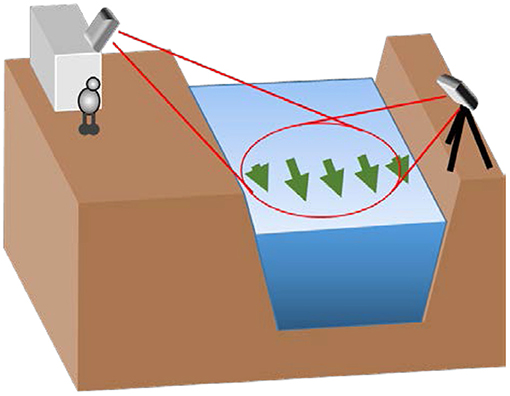
Figure 1. Schema of stream flow observations while acquiring images on river banks. The left side of the figure illustrates a camera fixed for continuous measurement and the right side shows a temporally located camera for event measurement.
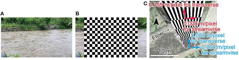
Figure 2. Examples of (A) an image taken at a side bank (853 by 480 pixels), (B) a 32 by 32 pixel grid overlaid on the image, and (C) an ortho-rectified 32 by 32 pixel grid. Quantities depicted using red and blue vectors indicate local resolution for the streamwise and transverse directions near the opposite side bank and the near side bank, respectively.
Here, we propose an approach of ortho-rectification that is free of limitations stemming from the degradation and distortion of image resolution. Overcoming this problem was a fundamental idea behind the methodological design of Space-Time Velocimetry (Fujita et al., 2007). Our study proposes an alternate approach for managing this problem by utilizing optical-system-based ortho-rectification. In System description, the proposed approach and system are explained. We employed an optical system embedded in an ultra-short throw projector. The proposed approach provides an ortho-rectified image during the image acquisition phase. Image resolution of the optically ortho-rectified image is almost uniform, in contrast to the highly inhomogeneous image resolution obtained from an ortho-rectified image using the conventional approach (see Figure 2C). In Field measurement, characteristics of the proposed approach used for field applications are validated and compared to those of the conventional approach. A summary and conclusions are provided in Summary and conclusions.
System Description
The optical system of a consumer-use image projector (produced for a mass market and publicly available with an affordable price relative to instruments produced for limited purposes) was used to optically ortho-rectify images. To record images using the optical system, the image display element, the source for the bright image pattern projected to the target surface, used in the projector was replaced with a complementary metal-oxide-semiconductor (CMOS) image sensor. The system is described in this section.
Optical System
For this study, the optical system of an ultra-short throw image projector, model LSPX-P1 (Sony Corporation, Japan), was utilized. Ultra-short throw image projectors project an image onto the plane orthogonal to the direction of the objective lens (see the left-bottom projector and the thin solid lines in Figure 3), whereas normal image projectors project an image almost directly in front of the objective lens (see the top projector and the dashed lines shown in Figure 3). The optical system used in this study was designed to cover 17 to 57 degrees of the depression angle. The left panel in Figure 4 shows the lens system extracted from the image projector. To obtain optically ortho-rectified images on the target plane, the 0.37-inch image display element was replaced with a CMOS image sensor (0.4-inch, MC500, Sanato, China). This particular sensor was used in this proof-of-concept study due to availability and cost. For future work, higher resolution sensors may also be employed. The right image of Figure 4 shows the captured image of a regular grid placed in front of the proposed system. Due to the unique characteristics of the optical system, the regular grid is highly distorted when the grid is placed in front of the objective lens of the device.
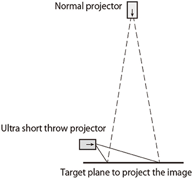
Figure 3. The optical paths of a standard projector (the dashed lines) and an ultra-short throw projector (the thin solid lines). For this study, an image of the target plane was received instead of the projector projecting (throwing) the image onto the target plane.
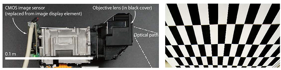
Figure 4. The optical system used in this study (left) and the image of the regular grid located in front of the camera (right).
Grid Pattern Test
For visualizing the characteristics of optical ortho-rectification, a grid pattern is placed on the floor. Figure 5 illustrates the spatial configuration of the grid pattern test. Figure 6A provides an image captured by the proposed system. Unlike images obtained from an oblique angle using a regular image capture system (see Figure 2 as an example), the grid pattern consists of 20 points with 0.25 m spacing, indicating almost regular and even spacing in the image as captured, without post-processing ortho-rectification. For obtaining a physical length for the image, scaling of the image should be determined.
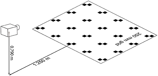
Figure 5. A schema of the image capturing configuration for the grid pattern test.
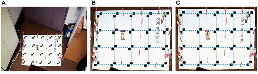
Figure 6. An example of grid pattern capture and calibration. (A) Image captured by the optical system. (B) Close-up of a grid in sub-figure (A). (C) Distortion and scaling corrected.
Figure 6B is an example of manual scaling based on the grid spacing provided. Manual scaling means that the exact regular grid (shown with blue lines) is overlain on the captured image to make it easy to visually confirm distortion within the grid of the captured image. Due to an imperfect optical setting, some skew in the image is observed, and grid points within the image do not completely match the regular and exact grid shown by the dashed blue lines in Figure 6B. In the region depicted in Figure 6B, the length error is roughly 1%. Length error and image skew are due to a misalignment of the camera orientation, causing image and coordinate distortion. Two approaches exist for correcting the scaling factor and camera orientation misalignment. The first approach involves using points in which the physical coordinates are known (ground control points, GCPs) in captured images, identifying parameters using general coordinate transform equations (introduced below), and correlating a pixel coordinate to the physical coordinate. The second approach involves specifying the coordinate transform equations using the camera's internal and external orientation parameters based on the relationship of the camera's physical coordinates and the target plane. The second approach can also be used with GCPs. For field measurements, the first approach is likely to be employed since the exact camera orientation and position are difficult to determine and are fixed. Therefore, a coordinate transform, a part of post-process methodology once an image has been captured using GCPs, is generally more flexible; and, by using an excess number of GCPs, the uncertainty of a coordinate transformation can be estimated. Figure 6C illustrates how distortion and scaling are corrected using the physical relationship of 20 grid points. The following general coordinate transform equations are used for the distortion and scaling correction (Tsubaki and Fujita, 2005):
here, x and y are the screen coordinates and are defined as (0, 0) at the screen center; X, Y and Z are the physical coordinates; a11 to a42 are the external camera parameters; and c and D are the internal camera parameters. The correction shown in Figure 6C is not perfect (e.g., estimates for the physical width of the domain shown in Figure 6C is 1.2 m and displacements of the left-bottom and the right-bottom grids in Figure 6C are 0.014 m for both the horizontal and vertical directions, thus the relative positional error can be estimated as 0.014 m/1.2 m = 1.2%). The error may be due to (1) imperfect setting of the optical system and (2) limitation using the general coordinate transform equations.
Field Measurement
Site Description
Video sequences were obtained using the proposed system during flushing discharge from a dam. The river section surveyed in our study is a side channel within the downstream reach of the Satsunai River, a tributary of the Tokachi River (Japan) system (Figure 7, Tsubaki et al., 2020; Zhu and Tsubaki, 2020). The Satsunai River Dam, a multipurpose dam (Figure 7B), discharged water. The event was surveyed during a flushing flow conducted on 24 June 2020. Figure 8 provides a hydrograph of discharge from the dam and the time-series change of water level recorded for the survey section (the location of the water level gauge is depicted as W.L. in Figure 7C). The discharge hydrograph consists of a 5.5 h rising phase and a 15 h falling phase. Peak discharge was approximately 110 m3/s. The video sequences discussed were obtained at 16:50, almost peak water level for the analyzed river section (Figure 8B). Water level was 1.75 m below the camera elevation at that time.
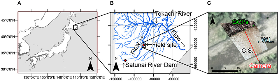
Figure 7. Location of the survey section. In the right panel, a distortion and scaling corrected image has been overlaid on an ortho-photo taken during 2019. GCPs correspond to ground control points. C.S. indicates the cross-section for the discharge calculation. W.L. indicates the location of water depth gauge settlement. (A) Location of the site. (B) Close-up around the site. (C) Ortho-photos of the site.
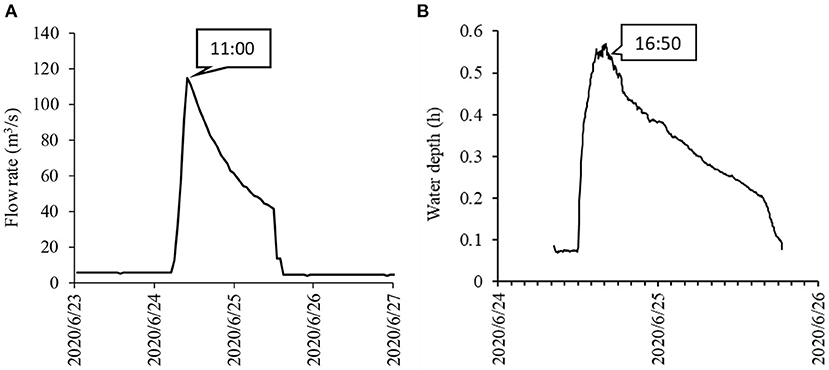
Figure 8. Flow rate and water depth hydrographs for the flushing flow event. (A) Discharging flow rate at the dam outlet. (B) Water depth at the survey section.
Video Sequences
The left photos in Figure 9 show snapshots of video sequences obtained during the survey. Figure 9A provides an image, with a resolution of 640 by 480 pixels and 30 frames per second, captured by the proposed optical system (left); and the image replaced by a 32 by 32 pixel grid (right). Figure 9B shows distortion and scaling for the corrected grid overlaid on the ortho-photo (right). The distorted grid in Figure 9B corresponds to how the original, evenly-spaced image resolution was distorted by the scaling and distortion correction described in Grid pattern test. If the system is installed in a specific geometry, the distortion in Figure 9B can be removed. For the field survey, due to changes in site geometry, placing the system in an exact geometry was difficult as a result of limited control for device orientation and limits to field measurement applicability. Therefore, assuming a distortion and scaling correction for images captured by the proposed system was reasonable for the field survey.
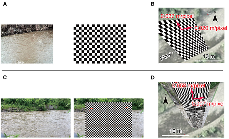
Figure 9. Captured snapshots (left), a 32 by 32 pixel grid overlay (middle), and images projected on the physical coordinate (right). Distorted grids in the right column indicate how local resolution of the original image (left) was deformed. Quantities depicted with red vectors in the right column indicate local resolution near the opposite side bank for the streamwise and transverse directions. (A) Image captured by the proposed system (640 by 480 pixel) (B) Distortion and scaling corrected image by the proposed system. (C) Conventional image (1920 by 1080 pixel). (D) Ortho-rectified image bythe conventional system.
While obtaining a video using the proposed system, another video sequence was obtained using a smartphone, a Sony Xperia XZ5. The image in the video obtained from the smartphone consisted of 1,920 by 1,080 pixels, with 29.97 frames per second. Image resolution obtained via the smartphone was finer than the image captured by the proposed system. To standardized image resolution to match the resolution obtained by the proposed optical system (640 by 480 pixels), a resolution-reduced image (853 by 480 pixels) set was made using the area average method. The obtained example is shown in Figure 2. Figure 9C displays the image set together with the original high-resolution image, and Figure 9D shows the ortho-rectified image of the high-resolution image.
When comparing images in the right column of each row in Figures 2, 9, the grid of the proposed system (Figure 9B) has less distortion as compared to the other data sets. Image resolution (physical length in meters per pixel for the captured image) for the streamwise and transverse directions was 0.020 m/pixel and 0.037 m/pixel, respectively (indicated with red vectors in Figure 9B). Local resolution for the streamwise and transverse directions depicted in Figures 2, 9 was calculated using the coordinate conversion equations [equations (1) to (5)]. The streamwise and transverse directions described here were exactly horizontal and vertical in image coordinates prior to ortho-rectification. Streamwise resolution for the conventional image with a reduced resolution (Figure 2C) was 0.020 m/pixel and was identical to those of the proposed system. However, resolution for the transverse direction was 0.155 m/pixel and was approximately four times coarser than that of the proposed system. Resolution for the streamwise direction of the image with an original image resolution (Figure 9D, 0.007 m/pixel) was approximately one-third of the value of the proposed system, owing to high resolution for the utilized image. Resolution of the transverse direction was, on the other hand, roughly two-fold of the proposed system, despite a high resolution for the image used. Reduced image resolution for the transverse direction occurs for ortho-rectification when an image is obtained from a small depression angle. By comparing image resolutions in Figures 2, 9, we can confirm that such a resolution reduction for the transverse direction was well-mitigated by the proposed system.
Particle Image Velocimetry
PIV Applied for Images Prior to Ortho-Rectification (PIV-First)
Particle image velocity (PIV) was used for estimating the water surface velocity distribution. An interrogation window size of 30 by 30 pixels was used for the low resolution image set (Figures 2, 9A); and 60 by 60 pixels was used for the high resolution image set (Figure 9C). Thirty-two frames were used and the peak location of the cross-correlation function amongst the pair of interrogation windows was calculated using a quadric fitting function for sub-pixel velocity estimation. First, an instantaneous velocity field for the captured image coordinates (prior to ortho-rectifying image coordinates) was calculated, and the mean velocity and standard deviation of the velocity fluctuation were calculated at each point aligned to a 32 pixel interval for the x and y directions in image coordinates. Velocity and velocity standard deviation vectors were then coordinate-transformed to physical coordinates (Tsubaki et al., 2018).
The velocity distribution in physical coordinates is plotted in Figure 10, using red arrows for the mean velocity and purple diamonds for the standard deviation. Noticeable from Figure 10 is that the density of the velocity vector near the opposite side bank is quite sparse for conventional approaches (Figures 10B,C). In contrast, the proposed approach provides an almost uniform velocity density and a high-resolution velocity distribution cover even near the opposite side bank (Figure 10A). For the proposed system (Figure 10A), the representative velocity magnitude was 2.39 m/s and the representative velocity standard deviation was 0.30 m/s. The representative velocity standard deviation corresponds to 12% of the velocity magnitude and is almost uniform in the domain. As confirmed by Figures 10B,C, velocity standard deviations for the velocity fields obtained from conventional procedures were more prominent in magnitude and more anisotropic for the spatial distribution. The mean velocity standard deviation was 0.43 m/s (18% with respect to 2.47 m/s) for the low resolution image set (Figure 10B), and 0.47 m/s (19% with respect to 2.41 m/s) for the high resolution image set (Figure 10C). Larger standard deviations for velocity obtained using conventional procedures result from reduced precision for instantaneous velocity estimations, due to a skewed water surface image. The standard deviation calculated from the measured velocity contains both measurement uncertainty and velocity fluctuation due to turbulence. The magnitude of water surface velocity fluctuations and/or the spatial scale of velocity fluctuations can be used, for example, for water depth and velocity index estimations (Johnson and Cowen, 2016). For such an analysis, precision for the instantaneous velocity distribution is required. A relatively small velocity standard deviation for the proposed system implies that the output of the proposed system contains less measurement uncertainty. Therefore, the proposed system provides a more precise velocity fluctuation as compared to the conventional procedure.
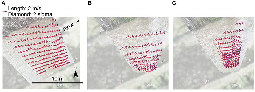
Figure 10. Distributions of the mean velocity (red arrows) and the standard deviation of the velocity (purple diamonds). The density of vectors for the conventional approaches were thinned during plotting to avoid overlying vectors. (A) Proposed system. (B) Conventional (low resolution). (C) Conventional (high resolution).
Undulation of the velocity distribution was observed at the channel center and near the opposite side bank. This type of undulation is caused by a standing-wave-like water surface undulation in elevation triggered by a three-dimensional flow structure. The apparent velocity undulation caused by irregularity of the water surface elevation is not a physical flow feature but, rather, a systematic measurement error. For managing this type of error, the shape of the water surface must be specified, and (1) a stereo imaging approach or (2) a separate measurement of water surface undulation is required. If an image is obtained perpendicular to the streamwise direction, as in this study, such a velocity error due to water surface three-dimensionality only appears for the transverse direction and does not affect the discharge estimation. As an alternative to the two approaches described above for managing the apparent velocity undulation problem, the multi-camera approach (Tsubaki, 2020) can also be used since, in the multi-camera approach, the erroneous transverse velocity component of each camera view is not used for reconstructing the velocity field.
PIV Applied for Ortho-Rectified Images (PIV-Later)
The proposed system records images with limited image distortion. The conventional system captures images with substantial coordinate distortion, and while using this approach, the normal protocol first includes ortho-rectifying images and then applying an image-based velocity estimation (Fujita et al., 1998, Perks, 2020). The advantage of this protocol is that the physical scale is easy to account for in the image based velocity estimation phase for highly coordinate-distorted cases. Such an advantage is not beneficial for the proposed system but may reduce substantial image resolution due to image interpolation. The upper sub-figures in Figure 11 compare the coordinate corrected images for the proposed and conventional systems. Resolution of the coordinate corrected (ortho-rectified) images were set to 0.02 m/pixel based on the representative pixel resolution of the captured images (Figure 9). To clarify the correspondence of pixels in captured and corrected images, here, no pixel interpolation was applied but the nearest neighbor algorithm was used when making these images. Vegetation on the bank was skewed in both the proposed and conventional cases due to vegetation's three-dimensionality, which was not well-treated in the simple coordinate transport model. The stepwise change of pixel color for the transverse direction is prominent in the image of the conventional system, whereas such an artifact was not confirmed in the image obtained from the proposed system. A stepwise change in pixel color was visually mitigated when pixel interpolation was used. However, a substantial resolution of information due to an image coordinate transformation could not, in essence, be mitigated.
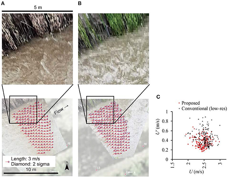
Figure 11. Distributions of the mean velocity (red arrows) and the standard deviation of the velocity (purple diamonds) obtained by ortho-rectified images. The close-ups of ortho-rectified images are depicted in the upper row. (A) Proposed system. (B) Conventional (low resolution). (C) Distributions of velocity magnitude and velocity standard deviation.
Lower plots shown in Figure 11 compare the distribution of mean velocity and standard deviation. The PIV setting was identical to that used in PIV applied for images prior to ortho-rectification (PIV-first). The representative velocity magnitude mean velocities were 2.43 m/s for the proposed system and 2.51 m/s for the conventional system. The mean velocity standard deviation magnitudes were 0.35 m/s and 0.44 m/s for the proposed and conventional systems, respectively. The mean velocity deviation magnitudes of the PIV-first were 0.30 m/s and 0.43 m/s for the proposed and conventional systems, respectively. When applying PIV-later, the velocity standard deviation increased by ~17% for the proposed system but was almost constant for the conventional method. For the proposed system, substantial image resolution may be reduced as a result of pixel manipulation among similar image resolutions, so the error in velocity estimation may be increased. Whereas, for the conventional method, the standard deviation was not changed because the pixel had been magnified so substantial image resolution had not deteriorated (nor improved) for such pixel upscaling processes. Figure 11C compares the plot of velocity magnitude and velocity standard deviation of each vector plotted in Figures 11A,B. The proposed system shows small scatter in both the standard deviation and velocity magnitude. This result implies the proposed system provides a more stable and uniform velocity distribution for both space and time than the conventional system.
The velocity profile showed undulation for both cases but was relatively evident in output obtained for the area close to the camera when using the conventional procedure. Results obtained using the proposed system were close for the opposite side bank. The former may be due to a larger uncertainty in the velocity estimation for the conventional procedure, while the latter could result because the velocity profile for the conventional procedure was affected by the peak locking effect.
Cross-Sectional Velocity Distribution and Discharge
Figure 12 shows the cross-sectional streamwise velocity distribution depicted in Figure 10 as well as the water depth distribution. Based on the two-dimensional, two-component velocity distribution, the velocity distribution perpendicular to the cross section was consolidated to the cross section (depicted as C.S. in Figure 7C). The cross section was divided into a one-meter interval, the mean water surface velocity component for each segment was then calculated and summed, and then a velocity index of 0.85 (e.g., Tsubaki et al., 2011) was multiplied to obtain the total discharge of a section. One sub-section closest to the near bank did not yield velocity data for the proposed and low-resolution conventional data, so velocity was interpolated using a neighboring velocity. When interpolating the velocity, assuming Manning's velocity equation, a ratio of 2/3 for the mean water depth power was employed. The obtained total discharge was 17.2 m3/s for the proposed optical system, 17.9 m3/s for the conventional procedure with a low resolution image set, and 17.5 m3/s for the conventional procedure with a high resolution image set. Differences amongst the three outputs was within 4%. Enormous velocity undulations and the velocity standard deviation did not significantly impact the discharge calculation.
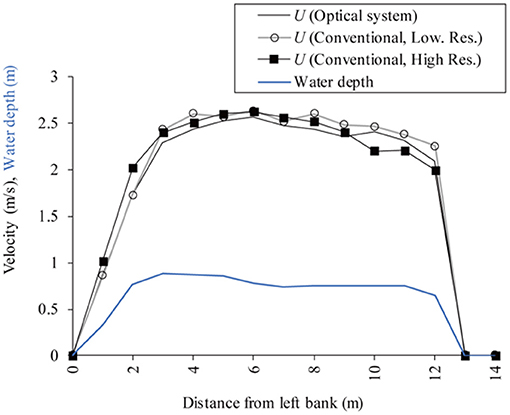
Figure 12. A cross-sectional distribution of streamwise velocity (the black lines) and local water depth (the blue line).
Summary and Conclusions
In the study, we proposed a new approach for managing the problem that arises from ortho-rectification and raster image manipulation. The proposed approach utilized an optical system for correlating the image coordinate to the physical coordinate. In System description, using the proposed system in the lab, the image obtained by the system without ortho-rectification during the post process had, roughly, a 1% length error. Coordinate distortion caused by the misalignment of camera orientations was not negligible, and coordinate transformation using the general coordinate transform equation and GCPs were applied. The proposed system was used for the field measurements provided in Field measurement. The two-dimensional, two-component velocity field of a channel was estimated using the proposed system and the conventional approach. The standard deviation of the local velocity time-series was reduced to 0.30 m/s, from 0.43 m/s, in output obtained from the conventional procedure, implying finer precision for the proposed system. The proposed system provided a more detailed two-dimensional, two-component velocity field as compared to conventional approaches due to a higher precision for the instantaneous velocity measurement with a higher substantial resolution in the area far from the camera. Local errors in instantaneous (random) and systematic (remains after averaging) velocity were not greatly impacted in the total discharge estimation.
Characteristics of the proposed approach were validated and compared to those of the conventional approach. However, data presented from this study is limited. Additional work will be undertaken for: (i) estimating exact and absolute errors in measurements, including the impact of water surface undulation on the obtained velocity field and the velocity standard deviation, (ii) more quantitatively understanding performance for the proposed approach, (iii) improving velocity measurement quality, and (iv) using coordinate transform equations for the scaling and misalignment correction, based on configurations of the optical system, including the necessity of a lens distortion model specific for the system.
Data Availability Statement
The raw data supporting the conclusions of this article will be made available by the authors, without undue reservation.
Author Contributions
RT contributed to conceptualization, methodological development, software development, and writing and revising the manuscript. RZ contributed to surveying, data collection, and data validation. All authors proofread the manuscript.
Funding
This study was supported by a research and development grant by the Foundation of River & Basin Integrated Communications (FRICS), Japan, and JSPS KAKENHI Grant Numbers 20H02257 and 21H01432.
Conflict of Interest
The authors declare that the research was conducted in the absence of any commercial or financial relationships that could be construed as a potential conflict of interest.
Publisher's Note
All claims expressed in this article are solely those of the authors and do not necessarily represent those of their affiliated organizations, or those of the publisher, the editors and the reviewers. Any product that may be evaluated in this article, or claim that may be made by its manufacturer, is not guaranteed or endorsed by the publisher.
References
Fujita, I., Muste, M., and Kruger, A. (1998). Large-scale particle image velocimetry for flow analysis in hydraulic engineering applications. J. Hydraulic Res. 36, 397–414. doi: 10.1080/00221689809498626
Fujita, I., Watanabe, H., and Tsubaki, R. (2007). Development of a non-intrusive and efficient flow monitoring technique: the space-time image Velocimetry (STIV). Int. J. River Basin Manage. 5, 105–114. doi: 10.1080/15715124.2007.9635310
Johnson, E. D., and Cowen, E. A. (2016). Remote monitoring of volumetric discharge employing bathymetry determined from surface turbulence metrics. Water Resour. Res. 52, 2178–2193. doi: 10.1002/2015WR017736
Kantoush, S. A., Schleiss, A. J., Sumi, T., and Murasaki, M. (2011). LSPIV implementation for environmental flow in various laboratory and field cases. J. Hydro-Environ. Res. 5, 263–276. doi: 10.1016/j.jher.2011.07.002
Le Coz, J., Hauet, A., Pierrefeu, G., Dramais, G., and Camenen, B. (2010). Performance of image-based velocimetry (LSPIV) applied to flash-flood discharge measurements in Mediterranean rivers. J. Hydrol. 394, 42–52. doi: 10.1016/j.jhydrol.2010.05.049
Muste, M., Fujita, I., and Hauet, A. (2008). Large-scale particle image velocimetry for measurements in riverine environments. Water Res. Res. 44:W00D19. doi: 10.1029/2008WR006950
Perks, M. (2020). KLT-IV v1.0: image velocimetry software for use with fixed and mobile platforms. Geosci. Model Dev. 13, 6111–6130. doi: 10.5194/gmd-13-6111-2020
Perks, M. T., Sasso, S. F. D., Hauet, A., Jamieson, E., Coz, J. L., Pearce, S., et al. (2020). Towards harmonisation of image velocimetry techniques for river surface velocity observations. Earth Syst. Sci. Data 12, 1545–1559. doi: 10.5194/essd-12-1545-2020
Tauro, F., Selker, J., Van De Giesen, N., Abrate, T., Uijlenhoet, R., Porfiri, M., et al. (2018). Measurements and observations in the XXI century (MOXXI): innovation and multi-disciplinarity to sense the hydrological cycle. Hydrol. Sci. J. 63, 169–196. doi: 10.1080/02626667.2017.1420191
Tsubaki, R. (2020). Multi-camera large-scale particle image velocimetry. Meas. Sci. Technol. 31:084004. doi: 10.1088/1361-6501/ab85d5
Tsubaki, R., Baranya, S., Muste, M., and Toda, Y. (2018). Spatio-temporal patterns of sediment particle movement on 2D and 3D bedforms. Exp. Fluids 59, 93_1–93_14. doi: 10.1007/s00348-018-2551-y
Tsubaki, R., Fuentes-Pérez, J. F., Kawamura, S., Tuhtan, J. A., and Sumitomo, K. (2020). Bedload Transport Measurement in a Japanese Gravel River Using Synchronized Hydrodynamic and Hydroacoustic Pressure Sensing, River Flow 2020. Boca Raton, FL: CRC Press.
Tsubaki, R., and Fujita, I. (2005). Stereoscopic measurement of a fluctuating free surface with discontinuities. Meas. Sci. Technol. 16:1894. doi: 10.1088/0957-0233/16/10/003
Tsubaki, R., Fujita, I., and Tsutsumi, S. (2011). Measurement of the flood discharge of a small-sized river using an existing digital video recording system. J. Hydro-Environ. Res. 5, 313–321. doi: 10.1016/j.jher.2010.12.004
Keywords: ortho-rectification, space-time image velocimetry, large-scale particle image velocimetry, optical system, ultra-short-throw projector
Citation: Tsubaki R and Zhu R (2021) Optical Ortho-Rectification for Image-Based Stream Surface Flow Observations Using a Ground Camera. Front. Water 3:700946. doi: 10.3389/frwa.2021.700946
Received: 27 April 2021; Accepted: 09 August 2021;
Published: 07 September 2021.
Edited by:
Matthew Perks, Newcastle University, United KingdomReviewed by:
Hojun You, IIHR-Hydroscience and Engineering, The University of Iowa, United States (Marian Muste, IIHR-Hydroscience and Engineering, The University of Iowa, United States, in collaboration with reviewer HY)Seth Schweitzer, Cornell University, United States
Guillaume Bodart, INRAE Clermont-Auvergne-Rhône-Alpes, France
Copyright © 2021 Tsubaki and Zhu. This is an open-access article distributed under the terms of the Creative Commons Attribution License (CC BY). The use, distribution or reproduction in other forums is permitted, provided the original author(s) and the copyright owner(s) are credited and that the original publication in this journal is cited, in accordance with accepted academic practice. No use, distribution or reproduction is permitted which does not comply with these terms.
*Correspondence: Ryota Tsubaki, cnRzdWJha2lAY2l2aWwubmFnb3lhLXUuYWMuanA=