Unprecedented Retention Capabilities of Extensive Green Roofs—New Design Approaches and an Open-Source Model

Green roofs are a proven measure to increase evapotranspiration at the expense of runoff, thus complementing contemporary stormwater management efforts to minimize pluvial flooding in cities. This effect has been quantified by numerous studies, ranging from experimental field campaigns to modeling experiments and even combinations of both. However, up until now, most green roof studies consider standard types of green roof dimensions, thus neglecting varying flow length in the substrate. For the first time, we present a comprehensive investigation of green roofs that involves artificial rainfall experiments under laboratory conditions (42 experiments in total). We consider varying flow length and slope. The novelty lies especially in the consideration of flow lengths beyond 5 m and non-declined roofs. This experimental part is complemented by numerical modeling, employing the open-source Catchment Modeling Framework (CMF). This is set-up for Darcy and Richards flow in the green roof and calibrated utilizing a multi-objective approach, considering both runoff and hydraulic head. The results demonstrate that through maximizing flow length and minimizing slope, the runoff coefficient (i.e., percentage of rainfall that becomes runoff) for a 100 years design rainfall is significantly decreased: from ~30% to values below 10%. These findings are confirmed through numerical modeling, which proves its value in terms of achieved model skill (Kling-Gupta Efficiency ranging from 0.5 to 0.95 with a median of 0.78). Both the experimental data and the numerical model are published as open data and open-source software, respectively. Thus, this study provides new insights into green roof design with high practical relevance, whilst being reproducible.

Introduction

Green roofs as a measure of green infrastructure play a key role in contemporary concepts to mitigate flooding in urban environments (van Hattum et al., 2016; Cascone, 2019). Concepts like water sensitive cities, sponge cities, low impact development (LID), and water sensitive urban design aim to mimic features of the natural water cycle, even in highly urbanized districts (Fletcher et al., 2015). For instance, green roofs reduce runoff and hence urban flooding due to their storage capacity. Evapotranspiration is also increased at the expense of runoff (Iffland et al., 2021), which better matches the characteristics of the natural water cycle. Moreover, green infrastructure (GI) in general, and green roofs in particular, provide important ecosystem services (Bolliger and Silbernagel, 2020), which demonstrates their value beyond storm water management. Through the linkage of evapotranspiration to the flux of latent heat, GI also play a key role in mitigating urban heat islands (Collier, 2016; van Hattum et al., 2016; Cirkel et al., 2018; Heusinger et al., 2018). Mitigating both urban flooding and urban heat islands is an important topic, since recent climate change suggests an intensification of short-term rainfall events that lead to urban flooding and longer heat waves. This in turn requires adequate climate change adaptation strategies (European Environment Agency, 2016). For instance, the past decades have seen an intensification of sub-daily rainfall events, which occur on time scales of minutes to a few hours (Förster and Thiele, 2020) and a further intensification is expected (Westra et al., 2014; Ban et al., 2015; Prein et al., 2017).

In the past decades, several experimental studies addressed the efficiency of green roofs in terms of runoff reduction, either as a response of artificial rainfall or actual rainfall. Hereby the former is done in the framework of indoor laboratory experiments, under idealized conditions, and the latter represents outdoor green roof installations, considering the long-term water balance. In Germany, runoff measurements with defined (artificial) design rainfall were carried out by Kolb (1987a,b, 1995, 1999, 2000), Liesecke (1988) and Liesecke and Lösken (1991), among others (Mendel, 1985; Liesecke, 1989; Schade, 2000, 2002). These results and scientific discussion were taken into account when the method for determining the runoff coefficient C (i.e., rainfall volume dived by runoff volume) was first specified in the FLL¹ Green Roof Guidelines (FLL, 2002). On the contrary, the peak discharge runoff coefficient C_s is used for the measuring of pipe diameters and the number of drains in roof drainage. To ensure comparability of results at different measurement sites, the guideline specified the area to be tested as 5 m long, 1 m wide with a 2% slope. At that time, this flow length corresponded to many common drainage lengths on roofs. Since the runoff coefficient C_s becomes smaller for longer flow lengths, the measurement design is safe even for longer flow lengths, since it tends to be oversized. In contrast, the measurements of annual water retention of natural precipitation are taken over a period of at least 4 years (Iffland et al., 2021). The tests for this purpose are carried out on test plots of 2 m × 2 m with a 2% slope, located outdoors and exposed to natural weather conditions. Schärer et al. (2020) compare peak discharge runoff coefficients measured in the laboratory with real runoff, from four roofs at different locations in Norway. In their research they deviate from the FLL Green Roof Guidelines (FLL, 2008, 2018) and instead irrigate the 2 m × 2 m experimental plots with a 2% slope in the laboratory, according to the method for determining the peak discharge runoff coefficient C_s, with a precipitation total of 27 mm over 15 min. Due to the short flow length, the peak discharge runoff coefficients are higher than if the measurements had been carried out according to the FLL Green Roof Guidelines. However, even though the effect of varying flow length has not been quantified in detail, the previous studies clearly demonstrate the retention capability of green roofs.

Consequently, green infrastructure in general and modeling the hydrology of green roofs in particular, increasingly gained attention in the past two decades (Li and Babcock, 2014). One well-known example is the Storm water Management Model (SWMM) which has been developed by the US Environmental Protection Agency (EPA) and is used worldwide (Rossman, 2010). SWMM is a conceptual rainfall-runoff model with hydrodynamic flow routing in sewer networks, designed for urban hydrology, which was complemented by GI/LID modeling capabilities. Several studies addressed the model component to model GI and more specifically green roofs (Burszta-Adamiak and Mrowiec, 2013; Cipolla et al., 2016; Krebs et al., 2016; Carson et al., 2017; Niazi et al., 2017; Peng and Stovin, 2017; Leimgruber et al., 2018; Limos et al., 2018; Liu and Chui, 2019; Iffland et al., 2021). For single green roofs, detailed physically-based models have been set up, utilizing models of the Hydrus family with different dimensions, ranging from 1D vertical modeling of the unsaturated zone (Hilten et al., 2008; Palla et al., 2008; Qin et al., 2016; Palermo et al., 2019; Mobilia and Longobardi, 2020) and two-dimensional cross-sections (Li and Babcock, 2015) up to three-dimensional representations of the green roof (Brunetti et al., 2016). Some authors even suggest to combine storm water modeling at the catchment scale using SWMM with Hydrus, in order to improve the representation of green roofs (Baek et al., 2020). Still, representing green roofs in models remains challenging in urban drainage modeling (Rosenzweig et al., 2021). Even though numerous studies successfully applied models to predict the hydrological response of green roof test plots, a major concern pertains to the transferability of parameters from one green roof configuration to another (Johannessen et al., 2019). Hence, parameters found through model calibration for a green roof test site equipped with measurement devices (which enable model calibration) might not be suitable to model similar green roof configurations without observations (Johannessen et al., 2019).

For this very reason, this study presents comprehensive artificial rainfall experiments, consisting of various green roof configurations with different combinations of maximum flow length and slope, for which a numerical model has been set up, with a unique parameterization valid for each configuration. The numerical model presented in this study also considers the explicit flow path to the outlet of green roofs, including saturated and unsaturated flow in the substrate as well as surface runoff, which is formed by ponding through rainfall excess at the surface. This feature is only rarely addressed up until now, given that most of the modeling studies in the literature utilize conceptual models or 1D vertical representations of flow processes in green roofs. Other models, like e.g., Hydrus, do not account for surface runoff. The availability of the model as free open-source software facilitates its applications in studies beyond the green roof scale.

Materials and Methods

Artificial Rainfall Experiments

Experimental Setup

The methodology for the artificial rainfall experiment was newly developed and is based on the experience gained from conducting experiments to determine the peak discharge runoff coefficient (C_s), according to the procedure specified in the FLL Green Roof Guidelines 2008 (new version 2018). For several variations, the experiments deviate from the established flow length of 5 m, the slope of 2% and the artificial design rainfall of 27 mm over 15 min (1.8 mm min⁻¹ or 300 l s⁻¹ ha⁻¹), in order to investigate the impact of flow length and slope. This artificial rainfall corresponds to a 100 years design storm in terms of intensity for the rainfall duration of 15 min (example for Hanover, Germany). This way, the experiments are designed to analyze the hydrological response of green roofs under extreme rainfall conditions.

The experiments were carried out in a greenhouse on the grounds of the Leibniz University Hannover (Germany), located at the Herrenhausen campus, on a 20 m runoff measuring track. The track consists of an assembly of four test plots, each 5 m in length, which are otherwise used for a number of other measurements, such as the determination of the runoff coefficient according to the FLL Green Roof Guidelines (2008, 2018). The connected plots allow for the studying of flow along a track 20 m in length and 1 m in width (see Figure 1). With four lifting devices, the 20 m track can be adjusted to different inclinations and thus also be without slope.

FIGURE 1

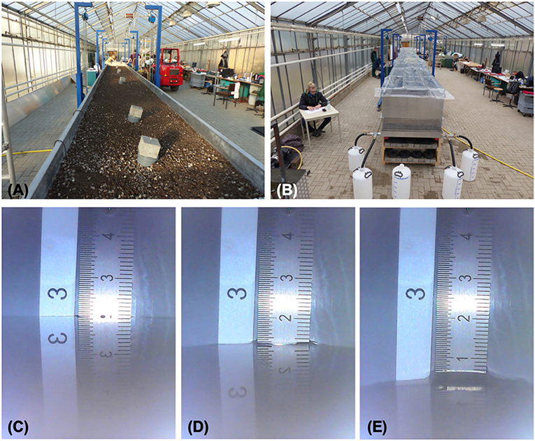
Figure 1. (A) Built-in layer setup with camera measuring points. (B) Enclosed test facility during artificial rainfall experiments. (C–E) Water levels recorded with endoscope cameras.

A protective fleece of 300 g/m² is installed as the bottom layer, which corresponds to the construction standard for extensive green roofs in Germany. On top of this, a single-layer substrate with a layer thickness of 8 or 10 cm is mounted, which in terms of water capacity and water permeability meets the requirements of the FLL Green Roof Guidelines (2008, 2018) for substrates for single-layer extensive green roofs. The investigations are carried out without vegetation on the surface. For the measurement of the water level (hydraulic head), the measurement track is instrumented with up to nine endoscope cameras, installed at different distances from the outflow. These cameras allow for continuous recording of the water level (see Figure 1). In order to show the influence of the individual layers of a green roof setup, additional artificial rainfall experiments with protective fleece and drainage mats are considered as well.

In each experiment, the measurement track is covered overnight to minimize evaporative loss (Figure 1). Due to its length, the entire test facility is located in a greenhouse with partial shading through paint, to reduce ambient temperatures in summer. The temperature was measured in the greenhouse as additional information. The endoscope recordings are started at the beginning of the experiments. In case of a 0% slope setup, an initial water level along the measurement sections is generally observed. This initial water table is the result of previous experiments, due to the low drainage rates along the measurement track. Declined experiments, with a slope of 2%, do not show this initial water table, since the drainage is more efficient in this case.

During the experiments, when the maximum scale of the endoscope recordings is reached, the water levels at the endoscope camera locations are also determined manually, at time intervals, using a millimeter scale. The design rainfall is applied utilizing a sprinkler system and the runoff is manually recorded at regular time intervals in collection tanks. Artificial rainfall with the sprinkler system is controlled by a calibrated water meter, checked every 30 s, and corrected if necessary. Sprinkling is done after pre-running built-up saturating sprinkling and 24-h dripping, at different intensities and flow lengths.

Description of Artificial Rainfall Experiments

In 2015, 2019, and 2020, a total of 99 sprinkler applications (artificial rainfall experiments) are carried out with different setups. In the following, only those experiments are considered that represent typical green roof structures (42 in total). The materials used are installed in accordance with the FLL Green Roof Guidelines (2008, 2018). The material properties, as well as the substrate characteristics, can be taken from the supplement (Supplementary Tables 2–6). The pore volume of the substrate (substrate 1: 60.5 Vol.-%; substrate 2: 53.5 Vol.-%), the maximum water capacity (substrate 1: 24.0 Vol.-%, substrate 2: 23.9 Vol.-%) as well as the permeability (substrate 1: 171.0 mm min⁻¹; substrate 2: 100.5 mm min⁻¹) are important for the simulations. Table 1 shows the setups investigated in the greenhouse, while Tables 2–4 (Results) compile the artificial rainfall experiments carried out in 2015, 2019, and 2020, respectively. The runoff behavior of extensive green roofs with 0% slopes was investigated in 2015, with the aim to quantify the problem of water retention in such green roofs (FBB, 2015).

TABLE 1

Table 1. Types of setups considered in the artificial rainfall experiments.

TABLE 2

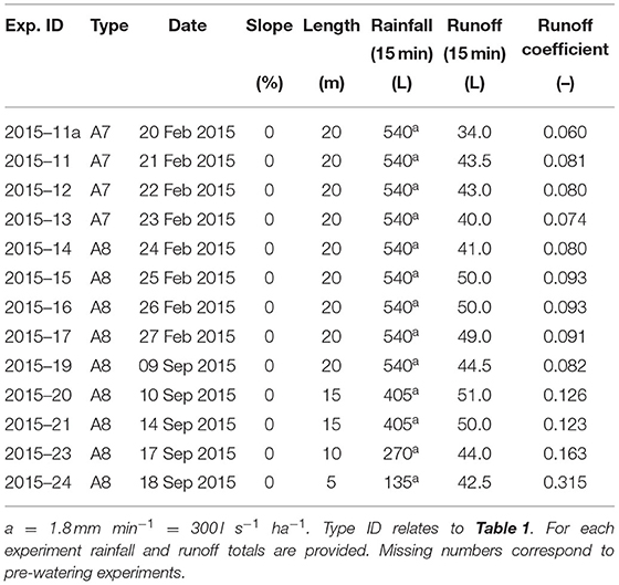
Table 2. Artificial rainfall experiments carried out in 2015 with 0% slope.

“Sprinkling the setup until uniform runoff is maintained over 10 min as a consequence of saturation” is a prerequisite (FLL, 2018, p. 130). However, a modified approach is considered here, in order to measure the runoff of a completely dry substrate setup and of a substrate setup forced with a design rainfall of a 100-year return period in Hannover Herrenhausen (27 mm within 15 min corresponding to 1.8 mm min⁻¹ or 300 l s⁻¹ ha⁻¹), after a time period of 24 h. The respective artificial rainfall experiments are then continued accordingly, after each 24 h, until three repetitions match approximately, in terms of runoff response (some specific deviations will later be explained separately). For the 3-fold repetitions, it is then possible to assume the same moisture situation in the substrate for the simulations. This is generally achieved after two artificial rainfall experiments. The artificial rainfall experiments after prolonged drought could assume extensive drying of the experimental setup. If there is a weekend between experiments, a 1-day pre-watering is deemed sufficient. The hydrological response for each artificial rainfall (sprinkler) experiment is compiled in Supplementary Figure 1. Pictures of the measuring track are shown in Supplementary Figures 2–6.

Limitations

The experiments were not originally designed to be addressed in modeling studies and hence adjustments have been introduced for this purpose, during the 2019 and 2020 implementation. Some test data from 2015 are therefore subject to limitations. For example, the water pressure and volume accuracy of the local pipe network were not sufficient for the experiments. Water was piped from a tank with a pump, through a water meter with a downstream stop valve and flow meter, so that flow could be manually increased or decreased. For extensive green roofs, the resulting inaccuracies do not affect the determination of the runoff coefficient according to the FLL Green Roof Guidelines, since the time series of the artificial rainfall corresponded well to the rainfall rate of the block rain, suggesting a constant rainfall intensity of time. For simulations, this can nevertheless be important, which is why simulations were carried out with the real artificial rainfall series and fluctuations resulted from readjustment during irrigation. This effect is particularly evident in the test sprinkling of the empty experimental system (Figure 2).

FIGURE 2

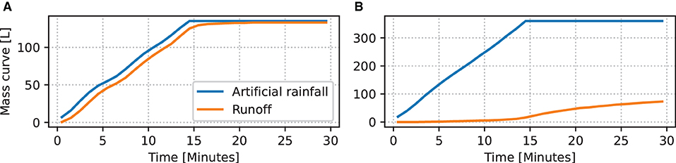
Figure 2. Mass curves of artificial rainfall and runoff for experiments (A) “empty test track” (no substrate) and (B) 2019–47 (substrate), respectively.

Numerical Model

Model Design

The numerical model is a fully connected two-dimensional representation of water flow through a longitudinal section in the substrate (Richards equation), and runoff at the substrate surface, with a diffusive wave approximation of the St. Venant equation. The partial differential flow equation of the water content continuum is discretized with a finite volume method, into a system of ordinary differential equations (ODE). The model is built using the Catchment Modeling Framework (CMF) by Kraft et al. (2011), in a setup comparable to the isotope transport hillslope model by Windhorst et al. (2014). The ODE—system representing the surface-subsurface flow continuum is integrated using a variable order multistep method with a banded Newton-Krylov preconditioner CVODE solver from the SUNDIALS 3.0 package (Hindmarsh et al., 2005). The model is composed using a Python script (Förster and Kraft, 2021) that utilizes the numerical framework of CMF. The mass balance for individual storages (nodes) is given by Equation 1:

$\begin{array}{ll}\frac{d{V}_i}{dt}={\displaystyle \sum _{j=1}^{N_i}}\left(-q_{i,j}\left(V_i,V_j,t\right)\right)& (1)\end{array}$

V is the volume of stored water in the control volume, i the current control volume, N the number of connected storages to i, q_i,j the flux in m³/day from i to j. The flux q is calculated for subsurface connections using the Darcy equation and the Richards equation, respectively, for variable saturated porous media:

$\begin{array}{ll}{q}_{i,j}=\frac{\Psi \left({\text{V}}_i\right)-\Psi \left({\text{V}}_j\right)}{d}·K\left(\theta \right)·A& (2)\end{array}$

With Ψ (V) as the function to calculate the pressure head and matric potential from the stored volume, d is the distance between the storage centers, K(θ) is the geometric mean hydraulic conductivity as a function of volumetric soil moisture θ between the storages, and A is the cross-section of the flux. For infiltration, Ψ (V) of the surface storage becomes the water level height.

The surface runoff is calculated using a diffusive wave with Manning friction:

$\begin{array}{ll}{q}_{i,j}=d{(V_1,V_2)}^{5/3}\sqrt{\frac{h(V_1)-h(V_2)}{d}}·n^{-1}& (3)\end{array}$

With d(V₁, V₂) the mean flow depth between V₁ and V₂, h the water level at the storage centers, d the distance between the storages and n the Manning roughness of the surface.

The rectangular grid for the construction of the finite volumes has a regular horizontal spacing of 0.2 m and vertical resolution of 0.02 m (Figure 3), and a not confined surface water storage at the top.

FIGURE 3

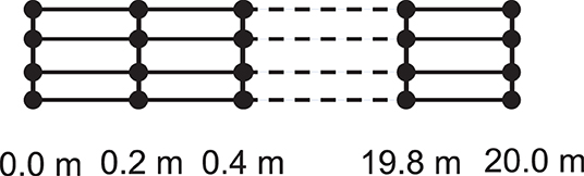
Figure 3. Numerical grid for green roofs realized in CMF.

A pore volume of 50% was assumed throughout the experiments, acknowledging that constructing the green roofs is always subject to substrate compaction. The water retention curve (i.e., the relation between volumetric water content and matric potential) is described using the Brooks-Corey retention curve. Surface flow on the roof top is modeled with a diffusive wave approximation setting the Manning's roughness coefficient to 0.08 (Maidment, 1993). Saturated conductivity and the curve-shape parameter b of the Brooks-Corey retention curve are calibrated parameters, as explained in the next section. The initial potential for the 0% slope experiments is set to −0.1 m (pF = 0.99) and −0.3 m (pF = 1.47) for the 2% experiments, respectively, to account for more complete drainage in the presence of a slope. Boundary conditions of the model are rainfall at the top, no flow condition at the right side and bottom and air potential at the left side.

Model Application

The model is applied to 42 of the 99 experiments, as described in Tables 2–4, if they meet the following properties: realistic initial water content, a substrate layer of at least 0.08 m thickness (other experiments also consider empty tracks, which are not considered here). The experiments 2015–19, 2019–28, 2019–43, and 2019–47 have been selected for model calibration, to estimate global optimal values for conductivity and the retention curve shape parameter, which are then applied to each experiment. These experiments represent the range of green roof configurations and rainfall intensities. The remaining 38 experiments are used to validate the model. This way, a split basin test is applied (Klemes, 1986).

A multi-objective calibration scheme is applied here, considering both runoff and hydraulic head. The objective functions to be maximized are

• Kling-Gupta Efficiency KGE (Gupta et al., 2009) for runoff and

• RMSE to Standard deviation ratio RSR (Moriasi et al., 2007) for hydraulic head.

An average value is computed out of both objective functions, whereby the negative values of RSR are used to compute the average values out of both values. The parameter optimization uses the Differential Evolution Adaptive Metropolis (DREAM) algorithm (Vrugt, 2016), implemented in “spotpy 1.5.8” by Houska et al. (2015). This way, the average computed out of KGE (runoff) and −RSR (hydraulic head) is maximized (in 172 iterations in total).

Results

Artificial Rainfall Experiments

The 2015 experimental focus was on the runoff behavior of extensive green roofs at a 0% slope (Table 2). The substrate layers generally introduce retention [up to 23 h to drain experiments (FBB, 2015)], resulting in low runoff coefficients, ranging from 0.06 at 20 m length to 0.315 at 5 m length for a design rainfall with 100 years return period. The shorter the flow length, the greater the runoff coefficient. Table 2 shows the runoff coefficients computed for each experiment, whereby the vertical extent of the substrate in the single-layer setup (setups A7 and A8) play a role in the runoff delay. For example, the runoff coefficient of 0.08 for a single-layer setup with 10 cm extensive substrate at a flow length of 20 m is very low, and can thus be rated as particularly good.

The experiments conducted in 2019 and 2020 focus on the influence of flow length and rainfall total at a 2% slope. Tables 3, 4 show that as rainfall decreases from 1.8 to 1.2 mm min⁻¹ (300 to 200 l s⁻¹ ha⁻¹), the runoff coefficients are also lower (experiments 2019–27 to 2020–62). It is interesting to note that the runoff coefficient at a 0% slope and 5 m flow length (2015–24) is higher than at approximately the same test set-up with a 2% slope (2019–40 to 2019–44 and 2020–60 to 2020–62). This is due to the residual water in the coarse pores before the start of the experiment, which drains overnight at a 2% slope and is still present in the substrate at 0% slope (FBB, 2015).

TABLE 3

Table 3. Artificial rainfall experiments carried out in 2019 with 2% slope.

TABLE 4

Table 4. Artificial rainfall experiments carried out in 2020 with 2% slope.

As with a 0% slope, it also holds for the 2% experiments that as the flow length to the outlet increases, the runoff coefficient decreases. For strong rainfall of 1.8 mm min⁻¹ from 0.207 (2019–43) to 0.170 (2019–28) and for reduced rainfall of 1.2 mm min⁻¹ from 0.106 (2020–61) to 0.042 (2020–49). Sprinkling in 2019–27, 2019–32, 2019–40, and 2020–46 is within the saturation phase of the setup, meaning multiple sprinklings were needed to reach full water saturation, depending on the date (this includes measurements not shown in 2019–31, 2019–35, and 2019–36, 2020–50, 2020–55, and 2020–59 and 2020–60).

During the sprinklings on 20 m flow length, water accumulation occurred that reached above the substrate surface. At 0% slope, the buildup proceeded slowly from the rear of the setup toward the front and ended about 1.25 m away from the outlet (e.g., measurement 2015–16; see Supplementary Figures 7–13 for pictures). This buildup can be explained by the water still standing from the measurement on the previous day (2015–15), since the water level in the substrate was higher in the rear area of the substrate than in the front area (water level at measurement 2015–16: camera 3 = 0.6 mm and at camera 8 = 13 mm). The closer the measurement location to the drain, the lower the water level was, before the start of sprinkling in the setups with a 0% slope.

The situation was different at a 2% slope: water accumulation occurred above the substrate surface in the front area, at 20 m flow length, during sprinkling. It occurred from the front to the back, whereby the accumulation stopped ~0.6 m before the outlet and the water in the substrate ran to the outlet (e.g., during the test run before measurement 2019–26; see Supplementary Figures 14, 15 for pictures; high water levels e.g., also during measurement 2019–28). Similarly, in the rear no ponding is observed. This ponding behavior is explained by the 2% slope, which provides faster runoff and thus increases water volumes on long flow lengths that are above the maximum flow of the installed green roof structure. The water accumulates and flows superficially.

Modeling

Figure 4 shows the results of the experiments selected for model calibration. The plots also include some relevant characteristics for each experiment, including dimensions, rainfall input, and the skill measures used to compute the objective function in the calibration procedure. KGE is computed from observed and modeled runoff time series and the RMSE is evaluated through comparing all pairs of observed and modeled hydraulic head along the x dimension (i.e., the longitudinal section). As a result of the optimization with DREAM in spotpy, the best run yields the following list of optimized parameters (2 in total): (i) saturated hydraulic conductivity of 1599 m d⁻¹ and (ii) Brooks-Corey b of 5.51. As described in Sect. Model Application, the multi-objective calibration procedure includes the experiments 2015–19, 2019–28, 2019–43, and 2019–47 (Figure 4). For these experiments, runoff and hydraulic head are considered to compute an objective function (average out of KGE for runoff and negative RSR for hydraulic head) which is maximized in each iteration of the DREAM algorithm.

FIGURE 4

Figure 4. Results of model calibration for the experiments (A) 2015–19, (B) 2019–28, (C) 2019–43, and (D) 2020–47. Each subplot shows time series of artificial rainfall (bars), observed runoff (plus symbol), and modeled time series (line). Moreover, dimensions, rainfall input, and skill measures used for computing the objective function are shown (RMSE computed for hydraulic head is given in centimeters).

The results highlight the very good agreement between model and observations, especially for the 20 m experiments forced with a design rainfall of 27 mm over 15 min (1.8 mm min⁻¹ or 300 l s⁻¹ ha⁻¹). For both experiments (2015–19 and 2019–28) KGE exceeds 0.8, indicating an overall well performing model. However, the RMSE computed for hydraulic head is better for the 2% roof (2019–28) compared to the 0% roof (2015–19). A closer look at the simulation of hydraulic head reveals that the model overestimates hydraulic head near the outlet (edge that drains the green roof) as shown in Figure 5. For most of time steps plotted in the longitudinal sections, the distribution of hydraulic head in the simulations between x = 0 m and x = 5 m is higher than the corresponding values recorded by the cameras. Still, the modeled and observed longitudinal sections of hydraulic head match in principle and the average RMSE computed through averaging the RMSE for each time step is 2 cm. It is worth noting that, besides the deficiencies outlined before, ponding of surface runoff is captured well in the simulations (green line in Figure 5).

FIGURE 5

Figure 5. Longitudinal section of observed and modeled hydraulic head for different time steps in the artificial rainfall experiment 2015–19 (0%, 20 m, 27 mm/15 min). RMSE computed for hydraulic head is indicated for each time step shown.

Similarly, Figure 6 visualizes the corresponding comparison for the modeled and observed distribution of hydraulic head for the 2% experiment (2019–28). In this case, modeled and observed values of hydraulic reflect a higher agreement, expressed by a lower RMSE (1.4 cm). The comparison between both experiments shows the differences in flow characteristics within the substrate. While in the 0% experiment, the side facing away the outlet (rear, right hand side) is subject to highest hydraulic head, the 2% experiment reflects another minimum of hydraulic head, which is conditioned by drainage due to gravity and higher surface runoff. In contrast, the 0% experiment has only a minimum and that is near the outlet at x = 0 m. Indeed, the 2% experiment shows a similar minimum at the outlet but differs from the 0% experiment through its arched shape (c.f., Supplementary Figures 7–15), which is confirmed by the model.

FIGURE 6

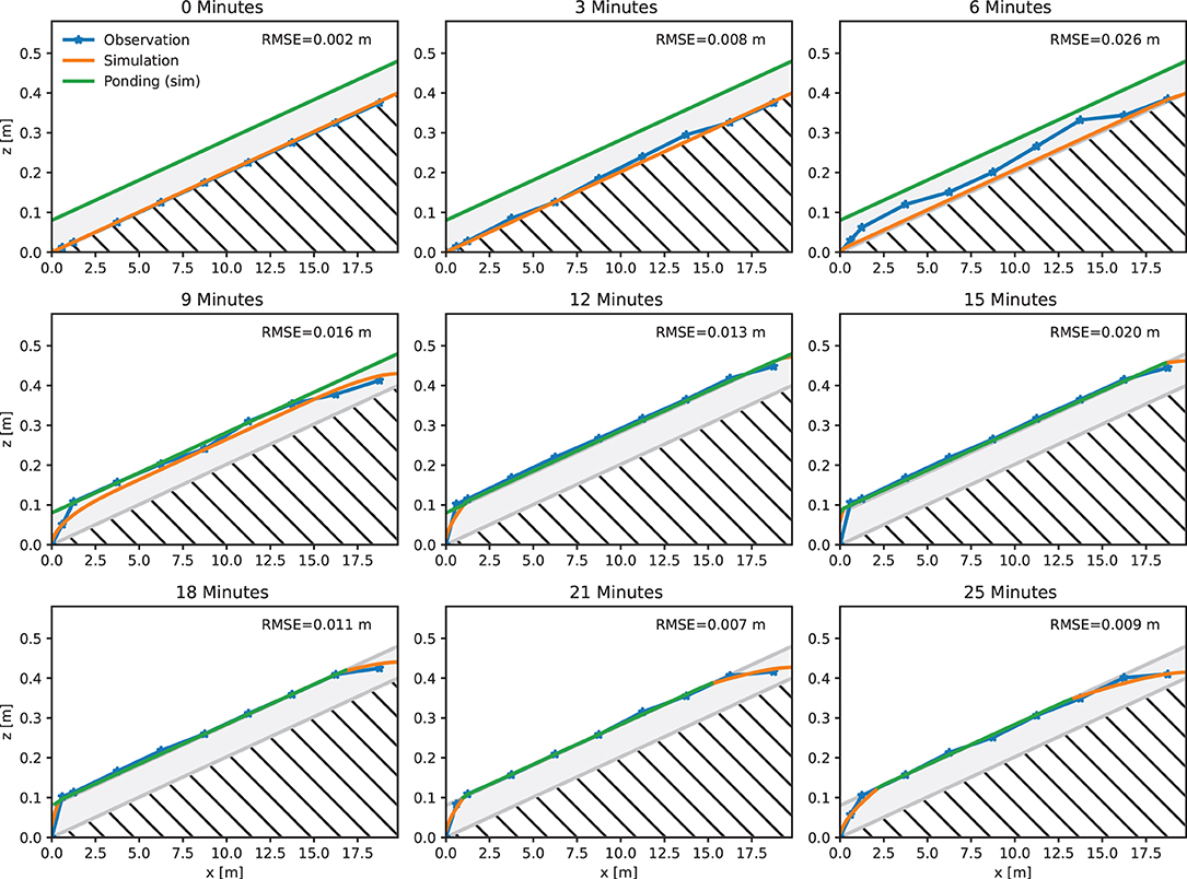
Figure 6. Longitudinal section of observed and modeled hydraulic head for different time steps in the artificial rainfall experiment 2019–28 (2%, 20 m, 27 mm/15 min). RMSE computed for hydraulic head is indicated for each time step shown.

The other two experiments utilized in the calibration period (i.e., 2019–43 and 2019–47) show lower model skill, in terms of both KGE (runoff) and RMSE (hydraulic head). However, RMSE is lowest for experiment 2019–43, even though KGE is slightly lower compared to 20 m experiments (2015–19 and 2019–28). In this experiment, the onset of the modeled runoff response occurs a few minutes earlier than the corresponding observation. However, the peak runoff achieved from the simulation is similar to the observed value, which confirms the accuracy found for the experiments 2015–19 and 2019–28. Among the experiments considered for calibration, the lowest model performance is found for experiment 2019–47. Both KGE and RMSE reflect deficiencies in terms of model accuracy. However, the rainfall forcing is smaller compared to the other three experiments and only amounts to 67% of the value in the remaining three experiments. It is worth mentioning that the subset of experiments considered in the framework of the calibration procedure are based on the same parameter set, even though different dimensions and rainfall volumes are considered. Moreover, initial moisture was unknown in experiments, which is why two start values (Methods) have been defined, one each for 0 and 2%, respectively. The lower model performance found for 2020–47 might be related to uncertainties associated with the estimation of initial conditions. However, the parameterization found through calibration is viewed acceptable, given the overall visual impression gained through comparing observation and simulation for each experiment.

In order to better justify the usage of this parameter set, an independent model validation is carried out. This way, all relevant experiments not considered in the calibration procedure are computed using the same unique parameter set. Figure 7, Supplementary Figure 1 and Supplementary Table 1 compile the results for all green roof experiments considered in the calibration and validation period. The way of displaying the results takes into account a differentiation according to the length of the green roof experiments (columns). In contrast, rows consider different sets of experiments in terms of slope (1st row 0%, starting from 2nd row 2%) rainfall volume (1st to 3rd row 27 mm/15 min, while the 4th row displays results of the 18 mm/15 min experiments).

FIGURE 7

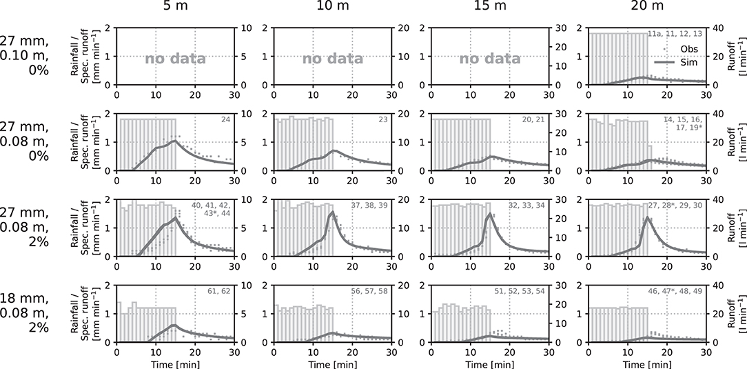
Figure 7. Observed and modeled runoff hydrographs for green roofs with different length (columns) as well as different slopes and rainfall forcing. Runs with asterisk denote experiments considered in the calibration procedure. The remaining experiments are modeled for validation purposes. The left y axis denotes specific runoff per unit area, similar to rainfall, while the right y axis allows for reading the total runoff. Rainfall is shown in form of bars, observed runoff is dotted and lines represent modeled runoff.

The comparison of modeled and observed runoff in each sub-panel highlights that the validation procedure confirms the validity of the parameter set found in the calibration procedure. Even though the experiments utilized for calibrating the model are included in the plot (marked with an asterisk), the number of experiments only used for validation purposes is much higher (38 vs. 4). Since the runoff hydrographs achieved by modeling match the corresponding observed values very well, the validation procedure suggests that the parameter set found through calibration is suitable to run the model for experiments not considered in the calibration procedure.

In order to complement the visual impression outlined in the previous statement with a quantitative statement, Figure 8 compiles box plots for a set of skill measurements computed for the experiments considered in the validation procedure. Here, the model runs used to calibrate the model are excluded. The box plot reflect that the results span a certain range of outcomes for each skill measure. For instance, for the Nash-Sutcliffe model efficiency and KGE, values are generally higher than 0.5, reflecting a reasonable model performance and even reach values beyond 0.9, which suggests a very good model performance. On average, the volume bias is around 0% and half the model runs are subject to volume bias of <15%. What might be responsible for this is that overestimations in terms of volume suggest too high initial moisture conditions and underestimations could be related to an underestimation of initial conditions, which again are unknown. The median of the RMSE, expressed as ratio to the corresponding standard deviation (RSR for runoff), is below 0.5, which is viewed an acceptable result (Moriasi et al., 2007). The Pearson correlation exceeding 0.9 in terms of the median value confirms the overall good model performance, especially highlighting that the correspondence in terms of timing is accurate. For hydraulic head, the distribution of RMSE values also suggests that the model is capable of representing the storage of water in the green roof. Fifty percent of the experiments show RMSE values between 1 and 2 cm, which is considered a reasonable accuracy, especially since reading the hydraulic head is also subject to limitations in terms of accuracy.

FIGURE 8

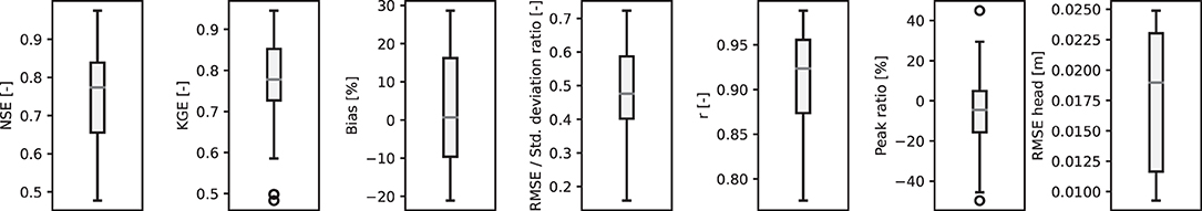
Figure 8. Box plots computed for all experiments considered in model validation including the following list of criteria: Nash-Sutcliffe Model efficiency (NSE), Kling Gupta efficiency (KGE), Percentage volume Bias, RMSE to Standard deviation ratio computed for runoff (RSR), Pearson correlation (r), RMSE for water level, as well as peak runoff ratio.

If one assumes that the parameter set is suitable for configurations not covered by the experiments used in the calibration procedure, the model is capable to represent the hydrological response of similar green roof configurations with arbitrary dimensions. This assumption is at least confirmed by the accuracy of model runs found in the validation period. Figure 9 shows the response surfaces for green roofs with different combinations of slope (x axis) and length (y axis). The rainfall forcing is 27 mm/15 min. The initial potential is set to −0.3 m for all runs here, to make the comparison independent of initial conditions². Sub-panel (A) visualizes the maximum specific peak runoff. For the rainfall forcing of 27 mm/15 min the theoretical maximum specific runoff amounts to 1.8 mm per minute, suggesting that the effect of retention is exhausted. The hydrological response in the plot suggests that this maximum specific runoff almost reaches this maximum value determined by rainfall for short flow length and higher slopes. Likewise, sub-panel (B) shows the retention expressed in terms of the runoff coefficient in the rationale method in hydrology (while the former is related to the peak discharge coefficient). Retention in terms of volume—as the runoff coefficient in the rationale method suggests—is more dependent on flow length, which is a measure of storage. In contrast, the relevance of reducing peak runoff is also determined by the slope. Even though both effects are not independent from each other, Figure 9 highlights the positive effect of both minimizing slope for reducing peak runoff and maximizing length for retention (and to a smaller degree for reducing peak runoff as well).

FIGURE 9

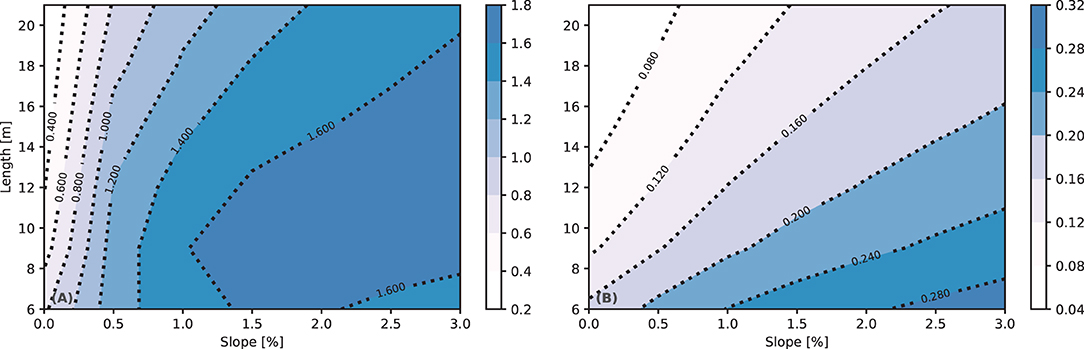
Figure 9. (A) Response surface for the specific peak discharge computed for different combinations of length and slope (mm min⁻¹). (B) Response surface showing computed runoff coefficients (t = 15 min) as a function of length and slope (–).

Discussion

For the experimental determination of the runoff coefficient at different flow lengths, the environmental conditions initially play a subordinate role. The peak runoff coefficient can still be determined according to the FLL Green Roof Guidelines (FLL, 2018), although a consideration of the flow length is decisive for the result. The runoff coefficient decreases with increasing flow length for single-layer green roofs and should be considered as another investigation possibility in the FLL Green Roof Guidelines in the future. Until then, the extended methodology should be based on the specifications of the FLL Green Roof Guidelines. The protective fleece that provides the bottom layer plays an important role here, since the greatest retarding effect is achieved here, especially in the case of long-term flow processes. On the other hand, when considering longer rainfall and runoff in models, the influence of the experimental environmental conditions is very important and this becomes noticeable very quickly, toward the end of a rainfall event. Evaporation of the setup over a longer period of time must be taken into account. Studying the role of different rainfall lengths and the impact of evaporation is beyond the scope of this article. However, considering both aspects explicitly is foreseen in future experiments. To this end, determination of substrate moisture prior to the start of experimental irrigation is also important. Monitoring of the entire experimental environment, or a climatic adjustment of the ambient space, is very costly and disproportionate, compared to the scenarios to be simulated. Simulating a real situation would also have limited availability of these parameters. Instead, the focus should be on simpler simulations that deviate further in detail but can represent the extreme case well, as this is important for the overloading of an overall system.

The low runoff coefficients of extensive green roofs with 0% slopes should be increasingly taken into account in quarter planning and urban drainage, since both the enormous storage capacity of up to two design rainfall events of a 100-year return period (example for Hanover), and the extremely slow runoff during rain events, speak for this. The design of 0% slope roofs without greening must be critically scrutinized from a structural engineering point of view, since puddles can form on the waterproofing, due to permissible construction tolerances, both in the execution planning and later in the construction. In the summer months, these water accumulations lead to temperature stresses at the edge of the puddle, which in turn stresses the waterproofing material and causes it to age more quickly. With extensive green roofs, the puddles are dissolved by the capillary action of the fleece, substrate and vegetation through evapotranspiration, while the greenery simultaneously ensures that temperatures in the moist substrate do not rise until the entire structure has dried out.

A numerical flow model is set-up for hydrological simulations of green roofs. Therefore, CMF is used to create a numerical model tailored to the experimental part of this study. One premise in model development was to carry out simulations for all experiments with a unique model structure and with a unique set of parameters. Only two parameters have been calibrated with a sophisticated optimization algorithm (DREAM) utilizing spotpy: hydraulic conductivity and Brooks-Corey b. The Brooks-Corey retention curve, with only one adjustable parameter, is a simplification. This is accepted here, since measuring the retention curve has not been considered in the experiments. Saturated hydraulic conductivity and the parameter b in the Brooks-Corey model have been altered by the optimization algorithm. The value b is related to pore size (Campbell, 1974; Tyler and Wheatcraft, 1990) and generally lower for coarse soils (or substrates), which justifies that b = 5.51 found through calibration is reasonable. According to Yates et al. (1992) the theoretical value of saturated conductivity is not directly related to matrix flow properties. This is why a potential around −0.05 m (pF = 0.69) is considered here, as reasonable guess to reflect the substrate's properties. The hydraulic conductivity at −0.05 m of K (−0.05 m) = 169 m d⁻¹ corresponds well to the value of K = 246 m d⁻¹ given by the manufacturer of the substrate. Another limitation is the fleece, which is not included in the model and thus its characteristics are implicitly included in the calibrated parameters. Apart from these limitations, it is still possible to provide the model with a more detailed representation of the water retention curve, in case measurements exist. For instance, if measurements of water content and matrix potential exist for the substrate, the water retention curve could be calibrated against these pairs of values.

The results also reflect that the model shows the highest accuracy for higher flow length and more intensive rain. This observation might also explain the slight decrease of peak runoff with decreasing length below ~7 m at higher slope values. Possible reasons for this mismatch might include a change in dominant processes, suggesting that surface runoff increases at the expense of Darcy flow for small flow length experiments. Since our study primarily focusses on flow length beyond the standard value of 5 m and design rainfall events, these limitations are viewed as acceptable. In essence, these results highlight that (i) CMF and more specifically the numerical model implementation in CMF represent the hydrology of the green roofs with high accuracy, and (ii) green roofs are a very efficient measure of green infrastructure that helps to reduce runoff. This holds even for design storms that are well-beyond return periods usually considered in urban drainage planning. This is especially relevant in the process of transforming gray to green infrastructure in light of climate change adaptation.

These findings are also of practical relevance: The occurrence of surface runoff is determined by the rainfall characteristics of the study site, the pore volume, and the material of the substrate. Vegetation onset counteracts erosion along the flow direction, which could be easily accomplished by mounting vegetation mats. This way, water prevailing in the substrate is also withdrawn through evapotranspiration, thus minimizing mass load on roofs. The decrease of the runoff coefficient, through maximizing the flow path in the substrate, could be taken into account in green roof drainage planning, e.g., through increasing the upside-down length or the catchment area per drain. For example, the partial drainage area size could be increased to 600 m² to 800 m² (instead of the generally planned 400 m² in Germany). The emergency drainage must be adjusted accordingly and also the statics of the roof would have to be taken into account. The extent to which larger flow lengths are possible would have to be investigated experimentally. Costs would thus be reduced and could be used for the professional design of the green roof.

Based on these findings and the discussion, the following recommendations can be made for designing green roofs and their design by means of models, respectively:

• Increase flow length in order to increase the upstream area (volume) connected to the roof drainage. This also suggests a longer time of concentration (flow or travel time, respectively);

• Consider non-declined green roofs, as this even reinforces the positive effect of increased flow length on both the time of concentration (and thus on retention) and mitigating rainfall peaks;

• Coupled modeling of sub-surface and surface hydrology of green roofs: In case of the 100 years design rainfall event considered here (example for Hanover), not only subsurface flow is observed. Instead, saturation excess at the surface (ponding) becomes a dominant process. An effective redistribution of water at the surface through surface runoff leads to downslope infiltration.

The first two recommendations suggest designing green roofs outside common standards. Therefore, we hope that our study helps to endorse new design approaches in future guidelines for the design of green roofs through a shift in paradigms. Indeed, this requires appropriate co-design of approaches to seal the bottom and to acknowledge building statics. Finally, the last recommendation addresses models as tools for planning green roofs. Complex interactions between surface and subsurface hydrology require physically based modeling approaches. The data and the model published alongside this article might help to guide both researchers and practitioners to achieve these goals.

Data Availability Statement

The datasets presented in this study can be found in online repositories. The names of the repository/repositories and accession number(s) can be found at: Westerholt and Lösken (2021); Förster and Kraft (2021).

Author Contributions

KF: modeling. DW: field campaign. PK: supervision of modeling. GL: supervision of the study. All authors contributed to discussing the results and writing the manuscript.

Funding

This research was funded by the Leibniz Universität Hannover. Parts of the 2015 campaign (experiments until February 2015) were funded by Fachvereinigung Bauwerksbegrünung (FBB), today Bundesverband GebäudeGrün e.V. (BuGG, German Association of Building Greening). The publication of this article was funded by the Open Access Fund of the Leibniz Universität Hannover.

Conflict of Interest

The authors declare that the research was conducted in the absence of any commercial or financial relationships that could be construed as a potential conflict of interest.

Publisher's Note

All claims expressed in this article are solely those of the authors and do not necessarily represent those of their affiliated organizations, or those of the publisher, the editors and the reviewers. Any product that may be evaluated in this article, or claim that may be made by its manufacturer, is not guaranteed or endorsed by the publisher.

Acknowledgments

We would like to thank several people who contributed to the success of this study. Firstly, the help of the student assistants and the administrative employees at the Institute of Landscape Architecture is greatly acknowledged: Sophie Beeskow, Laura Hahn, Marius Janning, Mira Ruben (in the 2015 campaign); Pia von Buttlar, Sophie Lange, Sina Mewes, Mira Ruben, Jelle Schacht, Gabriele Steinmeyer, Paul Struß (in the 2019/2020 campaign). Jonathan Westerholt developed the software for reading the camera recordings and helped to convert the data, which is greatly acknowledged. Lukas Bargel helped us to test an early version of the model. We wish to thank Larissa van der Laan for helping improve the English of the final version of this manuscript. Moreover, we would like to thank Martin Upmeier for the fruitful discussion on both the experimental and modeling results. Last but not least, the authors would also like to thank the reviewers for their comments which helped to improve the article.

Supplementary Material

The Supplementary Material for this article can be found online at: https://www.frontiersin.org/articles/10.3389/frwa.2021.689679/full#supplementary-material

Footnotes

1. ^Forschungsgesellschaft Landschaftsentwicklung Landschaftsbau is a research society for landscape development and landscaping in Germany. They publish green roof guidelines, which are primarily relevant for design in Germany but their guidelines have been also translated into English.

2. ^Please note: This is viewed a fair comparison, since prescribing a higher substrate moisture (−0.1 m) is only necessary to reconstruct the artificial rainfall experiments for non-declined green roofs in Figure 7. The reason for that is the daily interval of consecutive artificial rainfall experiments, which do not allow a complete drainage in case of non-declined setups (Section Model Design). Figure 9, however, reflects ideal conditions, not affected by this limitation arising from the experimental setup. Thus, both peak values and runoff coefficients for 0% in Figure 9 are lower than corresponding values presented in Tables 2–4 and Figure 7, respectively.

References

Baek, S., Ligaray, M., Pachepsky, Y., Chun, J. A., Yoon, K.-S., Park, Y., et al. (2020). Assessment of a green roof practice using the coupled SWMM and HYDRUS models. J. Environ. Manage. 261:109920. doi: 10.1016/j.jenvman.2019.109920

PubMed Abstract | CrossRef Full Text | Google Scholar

Ban, N., Schmidli, J., and Schär, C. (2015). Heavy precipitation in a changing climate: does short-term summer precipitation increase faster? Geophys. Res. Lett. 42, 1165–1172. doi: 10.1002/2014GL062588

CrossRef Full Text | Google Scholar

Bolliger, J., and Silbernagel, J. (2020). Contribution of connectivity assessments to green infrastructure (GI). ISPRS Int. J. Geo-Inf. 9:212. doi: 10.3390/ijgi9040212

CrossRef Full Text | Google Scholar

Brunetti, G., Šimunek, J., and Piro, P. (2016). A comprehensive analysis of the variably saturated hydraulic behavior of a green roof in a Mediterranean climate. Vadose Zone J. 15, 1–17. doi: 10.2136/vzj2016.04.0032

CrossRef Full Text | Google Scholar

Burszta-Adamiak, E., and Mrowiec, M. (2013). Modelling of green roofs' hydrologic performance using EPA's SWMM. Water Sci. Technol. 68, 36–42. doi: 10.2166/wst.2013.219

PubMed Abstract | CrossRef Full Text | Google Scholar

Campbell, G. S. (1974). A simple method for determining unsaturated conductivity from moisture retention data. Soil Sci. 117, 311–314. doi: 10.1097/00010694-197406000-00001

CrossRef Full Text | Google Scholar

Carson, T., Keeley, M., Marasco, D. E., McGillis, W., and Culligan, P. (2017). Assessing methods for predicting green roof rainfall capture: a comparison between full-scale observations and four hydrologic models. Urban Water J. 14, 589–603. doi: 10.1080/1573062X.2015.1056742

CrossRef Full Text | Google Scholar

Cascone, S. (2019). Green roof design: state of the art on technology and materials. Sustainability 11:3020. doi: 10.3390/su11113020

CrossRef Full Text | Google Scholar

Cipolla, S. S., Maglionico, M., and Stojkov, I. (2016). A long-term hydrological modelling of an extensive green roof by means of SWMM. Ecol. Eng. 95, 876–887. doi: 10.1016/j.ecoleng.2016.07.009

CrossRef Full Text | Google Scholar

Cirkel, D., Voortman, B., van Veen, T., and Bartholomeus, R. (2018). Evaporation from (Blue) Green Roofs: assessing the benefits of a storage and capillary irrigation system based on measurements and modeling. Water 10:1253. doi: 10.3390/w10091253

CrossRef Full Text | Google Scholar

Collier, C. G., (ed.). (2016). “Hydrometeorology in the urban environment,” in Hydrometeorology (Chichester: John Wiley and Sons, Ltd), 318–335.

European Environment Agency (2016). Urban Adaptation to Climate Change in Europe 2016: Transforming Cities in a Changing Climate. Luxembourg: Publications Office of the European Union. Available online at: http://bookshop.europa.eu/uri?target=EUB:NOTICE:THAL16011:EN:HTML (accessed January 3, 2019).

FBB (2015). Abschlussbericht zum Forschungsauftrag “Untersuchungen des Wasserabflusses bei Extensiven Dachbegrünungen bei einer Dachneigung von Null Grad”—Fachvereinigung Bauwerksbegrünung (FBB). Available online at: https://www.gebaeudegruen.info/fileadmin/website/downloads/bugg-untersuchungen/FBBForschungsberichtNullGradVulkatec.pdf

Fletcher, T. D., Shuster, W., Hunt, W. F., Ashley, R., Butler, D., Arthur, S., et al. (2015). SUDS, LID, BMPs, WSUD and more—the evolution and application of terminology surrounding urban drainage. Urban Water J. 12, 525–542. doi: 10.1080/1573062X.2014.916314

CrossRef Full Text | Google Scholar

FLL (2002). Dachbegrünungsrichtlinien—Richtlinien für die Planung, Bau und Instandhaltungen von Dachbegrünungen (Green Roof Guidelines. Guidelines for the Planning, Construction and Maintenance of Green Roofs). Bonn: Forschungsgesellschaft Landschaftsentwicklung Landschaftsbau e. V.

FLL (2008). Dachbegrünungsrichtlinien—Richtlinien für die Planung, Bau und Instandhaltungen von Dachbegrünungen (Green Roof Guidelines. Guidelines for the Planning, Construction and Maintenance of Green Roofs). Bonn: Forschungsgesellschaft Landschaftsentwicklung Landschaftsbau e. V.

FLL (2018). Dachbegrünungsrichtlinien—Richtlinien für die Planung, Bau und Instandhaltungen von Dachbegrünungen (Green Roof Guidelines. Guidelines for the Planning, Construction and Maintenance of Green Roofs). Bonn: Forschungsgesellschaft Landschaftsentwicklung Landschaftsbau e. V.

Förster, K., and Kraft, P. (2021). Green Roof—A Physically Based Flow Model for Green Roofs. Zenodo. doi: 10.5281/zenodo.4635675

CrossRef Full Text | Google Scholar

Förster, K., and Thiele, L.-B. (2020). Variations in sub-daily precipitation at centennial scale. npj Clim. Atmos. Sci. 3, 1–7. doi: 10.1038/s41612-020-0117-1

CrossRef Full Text | Google Scholar

Gupta, H. V., Kling, H., Yilmaz, K. K., and Martinez, G. F. (2009). Decomposition of the mean squared error and NSE performance criteria: implications for improving hydrological modelling. J. Hydrol. 377, 80–91. doi: 10.1016/j.jhydrol.2009.08.003

CrossRef Full Text | Google Scholar

Heusinger, J., Sailor, D. J., and Weber, S. (2018). Modeling the reduction of urban excess heat by green roofs with respect to different irrigation scenarios. Build. Environ. 131, 174–183. doi: 10.1016/j.buildenv.2018.01.003

CrossRef Full Text | Google Scholar

Hilten, R. N., Lawrence, T. M., and Tollner, E. W. (2008). Modeling stormwater runoff from green roofs with HYDRUS-1D. J. Hydrol. 358, 288–293. doi: 10.1016/j.jhydrol.2008.06.010

CrossRef Full Text | Google Scholar

Hindmarsh, A. C., Brown, P. N., Grant, K. E., Lee, S. L., Serban, R., Shumaker, D. E., et al. (2005). SUNDIALS: suite of non-linear and differential/algebraic equation solvers. ACM Trans. Math. Softw. 31, 363–396. doi: 10.1145/1089014.1089020

CrossRef Full Text | Google Scholar

Houska, T., Kraft, P., Chamorro-Chavez, A., and Breuer, L. (2015). SPOTting model parameters using a ready-made python package. PLoS ONE 10:e0145180. doi: 10.1371/journal.pone.0145180

PubMed Abstract | CrossRef Full Text | Google Scholar

Iffland, R., Förster, K., Westerholt, D., Pesci, M. H., and Lösken, G. (2021). Robust vegetation parameterization for green roofs in the EPA stormwater management model (SWMM). Hydrology 8:12. doi: 10.3390/hydrology8010012

CrossRef Full Text | Google Scholar

Johannessen, B. G., Hamouz, V., Gragne, A. S., and Muthanna, T. M. (2019). The transferability of SWMM model parameters between green roofs with similar build-up. J. Hydrol. 569, 816–828. doi: 10.1016/j.jhydrol.2019.01.004

CrossRef Full Text | Google Scholar

Klemes, V. (1986). Operational testing of hydrological simulation models. Hydrol. Sci. J. 31, 13–24. doi: 10.1080/02626668609491024

CrossRef Full Text | Google Scholar

Kolb, W. (1987a). Abflußverhältnisse extensiv begrünter Flachdächer—Abflußspenden und Wasserrückhaltung im Vergleich mit Kiesdächern. Z. Für Veg. 10, 111–116.

Kolb, W. (1987b). Wirkung des Sättigungsgrades der Vegetationsschicht auf Abflußspenden und Wasserrückhaltung. Z. Für Veg. 10, 162–165.

Kolb, W. (1995). Regenwasserabflüsse bei Grünflächen auf Dächern. Neue Landsch. 12, 901–903.

Kolb, W. (1999). Einflüsse der Oberfächenneigung auf die Abflußverhältnisse von Gründächern. Dach Grün 1, 4–8.

Kolb, W. (2000). Begrünte Dächer wirken wie Regenrückhaltebecken. Neue Landsch. 1, 31–33.

Kraft, P., Vaché, K. B., Frede, H.-G., and Breuer, L. (2011). CMF: a hydrological programming language extension for integrated catchment models. Environ. Model. Softw. 26, 828–830. doi: 10.1016/j.envsoft.2010.12.009

CrossRef Full Text | Google Scholar

Krebs, G., Kuoppamäki, K., Kokkonen, T., and Koivusalo, H. (2016). Simulation of green roof test bed runoff: simulation of green roof test bed runoff. Hydrol. Process. 30, 250–262. doi: 10.1002/hyp.10605

CrossRef Full Text | Google Scholar

Leimgruber, J., Krebs, G., Camhy, D., and Muschalla, D. (2018). Sensitivity of model-based water balance to low impact development parameters. Water 10:1838. doi: 10.3390/w10121838

CrossRef Full Text | Google Scholar

Li, Y., and Babcock, R. W. (2014). Green roof hydrologic performance and modeling: a review. Water Sci. Technol. 69, 727–738. doi: 10.2166/wst.2013.770

PubMed Abstract | CrossRef Full Text | Google Scholar

Li, Y., and Babcock, R. W. (2015). Modeling hydrologic performance of a green roof system with HYDRUS-2D. J. Environ. Eng. 141:04015036. doi: 10.1061/(ASCE)EE.1943-7870.0000976

CrossRef Full Text | Google Scholar

Liesecke, H.-J. (1988). Untersuchung zur Wasserrückhaltung bei extensiv begrünten Flachdächern. Z. Für Veg. 11, 56–66.

Liesecke, H.-J. (1989). Wasserrückhaltung und Abflußspende bei Extensivbegrünungen auf Flachdächern. Bundesbaublatt 38, 176–183.

Liesecke, H.-J., and Lösken, G. (1991). Dränung bei extensiven Dachbegrünungen. Gartenamt 40, 314–320.

Limos, A. G., Mallari, K. J. B., Baek, J., Kim, H., Hong, S., and Yoon, J. (2018). Assessing the significance of evapotranspiration in green roof modeling by SWMM. J. Hydroinformatics 20, 588–596. doi: 10.2166/hydro.2018.130

CrossRef Full Text | Google Scholar

Liu and Chui (2019). Evaluation of Green roof performance in mitigating the impact of extreme storms. Water 11:815. doi: 10.3390/w11040815

CrossRef Full Text | Google Scholar

Maidment, D. (1993). Handbook of Hydrology. New York, NY: McGraw-Hill.

Mendel, H. G. (1985). Die Bedeutung von Gründächern insbesondere aus wasserwirtschaftlicher Sicht. Gartenamt 34, 574–581.

Mobilia, M., and Longobardi, A. (2020). Impact of rainfall properties on the performance of hydrological models for green roofs simulation. Water Sci. Technol. 81, 1375–1387. doi: 10.2166/wst.2020.210

PubMed Abstract | CrossRef Full Text | Google Scholar

Moriasi, D. N., Arnold, J. G., van Liew, M. W., Bingner, R. L., Harmel, R. D., and Veith, T. L. (2007). Model evaluation guidelines for systematic quantification of accuracy in watershed simulations. Trans. ASABE 50, 885–900. doi: 10.13031/2013.23153

CrossRef Full Text | Google Scholar

Niazi, M., Nietch, C., Maghrebi, M., Jackson, N., Bennett, B. R., Tryby, M., et al. (2017). Storm water management model: performance review and gap analysis. J. Sustain. Water Built Environ. 3:04017002. doi: 10.1061/JSWBAY.0000817

PubMed Abstract | CrossRef Full Text | Google Scholar

Palermo, S. A., Turco, M., Principato, F., and Piro, P. (2019). Hydrological effectiveness of an extensive green roof in Mediterranean climate. Water 11:1378. doi: 10.3390/w11071378

CrossRef Full Text | Google Scholar

Palla, A., Lanza, L. G., and Barbera, P. L. (2008). “A green roof experimental site in the Mediterranean climate,” in 11th International Conference on Urban Drainage (Edinburgh), 1–10.

PubMed Abstract | Google Scholar

Peng, Z., and Stovin, V. (2017). Independent validation of the SWMM green roof module. J. Hydrol. Eng. 22:04017037. doi: 10.1061/(ASCE)HE.1943-5584.0001558

CrossRef Full Text | Google Scholar

Prein, A. F., Rasmussen, R. M., Ikeda, K., Liu, C., Clark, M. P., and Holland, G. J. (2017). The future intensification of hourly precipitation extremes. Nat. Clim. Change 7, 48–52. doi: 10.1038/nclimate3168

CrossRef Full Text | Google Scholar

Qin, H., Peng, Y., Tang, Q., and Yu, S.-L. (2016). A HYDRUS model for irrigation management of green roofs with a water storage layer. Ecol. Eng. 95, 399–408. doi: 10.1016/j.ecoleng.2016.06.077

CrossRef Full Text | Google Scholar

Rosenzweig, B. R., Cantis, P. H., Kim, Y., Cohn, A., Grove, K., Brock, J., et al. (2021). The value of Urban flood modeling. Earths Future 9:e2020EF001739. doi: 10.1029/2020EF001739

CrossRef Full Text | Google Scholar

Rossman, L. A. (2010). Modeling low impact development alternatives with SWMM. J. Water Manag. Model. 167–182. doi: 10.14796/JWMM.R236-11

CrossRef Full Text | Google Scholar

Schade, C. (2000). Wasserrückhaltung und Abflussbeiwerte bei dünnschichtigen Extensivbegrünungen. Stadt Grün 49, 95–100.

Schade, C. (2002). Eigenschaften und Anwendung von Vegetationsmatten in der extensiven Dachbegrünung—Beiträge zur Räumlichen Planung. Hannover: Schriftenreihe des Fachbereichs Landschaftsarchitektur und Umweltentwicklung der Universität Hannover.

Schärer, L. A., Busklein, J. O., Sivertsen, E., and Muthanna, T. M. (2020). Limitations in using runoff coefficients for green and gray roof design. Hydrol. Res. 51, 339–350. doi: 10.2166/nh.2020.049

CrossRef Full Text | Google Scholar

Tyler, S. W., and Wheatcraft, S. W. (1990). Fractal processes in soil water retention. Water Resour. Res. 26, 1047–1054. doi: 10.1029/WR026i005p01047

CrossRef Full Text | Google Scholar

van Hattum, T., Blauw, M., Jensen, M. B., and de Bruin, K. (2016). Towards Water Smart Cities: Climate Adaptation is a Huge Opportunity to Improve the Quality of Life in Cities. Wageningen: Wageningen University and Research. Available online at: http://library.wur.nl/WebQuery/wurpubs/fulltext/407327 (accessed September 20, 2017).

Vrugt, J. A. (2016). Markov chain Monte Carlo simulation using the DREAM software package: theory, concepts, and MATLAB implementation. Environ. Model. Softw. 75, 273–316. doi: 10.1016/j.envsoft.2015.08.013

CrossRef Full Text | Google Scholar

Westerholt, D., and Lösken, G. (2021). Artificial Rainfall Experiments for Green Roofs Depending on the Flow Length at 0% and 2% Slope and Different Rain Intensities (Version 1) [Data set]. Zenodo. doi: 10.5281/zenodo.4651339

CrossRef Full Text | Google Scholar

Westra, S., Fowler, H. J., Evans, J. P., Alexander, L. V., Berg, P., Johnson, F., et al. (2014). Future changes to the intensity and frequency of short-duration extreme rainfall. Rev. Geophys. 52, 522–555. doi: 10.1002/2014RG000464

CrossRef Full Text | Google Scholar

Windhorst, D., Kraft, P., Timbe, E., Frede, H.-G., and Breuer, L. (2014). Stable water isotope tracing through hydrological models for disentangling runoff generation processes at the hillslope scale. Hydrol. Earth Syst. Sci. 18, 4113–4127. doi: 10.5194/hess-18-4113-2014

CrossRef Full Text | Google Scholar

Yates, S., Van Genuchten, M. T., Warrick, A., and Leij, F. (1992). Analysis of measured, predicted, and estimated hydraulic conductivity using the RETC computer program. Soil Sci. Soc. Am. J. 56, 347–354. doi: 10.2136/sssaj1992.03615995005600020003x

CrossRef Full Text | Google Scholar