Macroscopic Model for Passive Mass Dispersion in Porous Media Including Knudsen and Diffusive Slip Effects

In this work, a macroscopic model for incompressible and Newtonian gas flow coupled to Fickian and advective transport of a passive solute in rigid and homogeneous porous media is derived. At the pore-scale, both momentum and mass transport phenomena are coupled, not only by the convective mechanism in the mass transport equation, but also in the solid-fluid interfacial boundary condition. This boundary condition is a generalization of the Kramers-Kistemaker slip condition that includes the Knudsen effects. The resulting upscaled model, applicable in the bulk of the porous medium, corresponds to: 1) A Darcy-type model that involves an apparent permeability tensor, complemented by a dispersive term and 2) A macroscopic convection-dispersion equation for the solute, in which both the macroscopic velocity and the total dispersion tensor are influenced by the slip effects taking place at the pore-scale. The use of the model is restricted by the starting assumptions imposed in the governing equations at the pore scale and by the (spatial and temporal) constraints involved in the upscaling process. The different regimes of application of the model, in terms of the Péclet number values, are discussed as well as its extents and limitations. This new model generalizes previous attempts that only include either Knudsen or diffusive slip effects in porous media.

1. Introduction

Gas flow in porous media is a relevant topic that has attracted intense research over, at least, the past 50 years (see, for instance, Jackson, 1977; Ho and Webb, 2006). The flow process may be coupled to heat and also to species mass transport, which makes it of major interest in a wide variety of practical situations including: crystal growth from vapor, chemical processes in porous catalysts, material processing using chemical vapor infiltration or deposition, exploitation of natural gas and oil, CO₂ sequestration, micro electro-mechanical systems, shale gas flow in nanoporous media, long-term nuclear waste disposal, contaminant transport in underground formations, gas separation with permeable media, among many others (Rutherford and Do, 1999; Cai et al., 2007; Li et al., 2019; Tian et al., 2019; Barton, 2020; Wang et al., 2020).

Under single-phase and isothermal flow conditions, gas slip may result from either Knudsen effects (also referred to as viscous slip) (Navier, 1823; Einzel et al., 1990) or diffusive slip (Kramers and Kistemaker, 1943; Jackson, 1977; Noever, 1990; Young and Todd, 2005). The first type of slip leads to the Klinkenberg (1941) modification to Darcy's law in porous media (Skjetne and Auriault, 1999; Lasseux et al., 2014, 2016; Woignier et al., 2018) as well as in fractures (Zaouter et al., 2018) and it is only coupled to mass transport by means of convection (Valdés-Parada et al., 2019). A comprehensive review about modeling gas flow in porous media considering Knudsen slip is available from Lasseux and Valdés-Parada (2017). The second type of slip boundary condition leads to a modification to Darcy's law that involves the macroscopic mass flux, whereas the macroscopic mass equation is more complicated than the classical convection-dispersion model as shown by Altevogt et al. (2003a) for dilute solutions and more recently by Moyne et al. (2020) for multispecies concentrated solutions. Despite these considerable advances, it is possible to encounter in practice situations in which both types of slip effects are present. For example, one may envisage species transport in a porous medium where diffusive slip is relevant and for which the Knudsen number value is not extremely small compared to 1 (i.e., on the order of 0.1) so that viscous slip must also be considered. To the best of our knowledge, modeling of this problem at the different scales of interest has not been addressed so far and the upscaled model corresponding to this situation has not yet been reported in the literature. When both slip effects are considered, the pore-scale model is nonlinear due to the coupling with mass transport at the solid-fluid interface. Hence, the question remains whether the resulting upscaled model is a superposition of the existing ones considering the two slip effects separately.

The rationality of the present work is hence to derive an upscaled model for momentum and total and species mass transport involving both Knudsen and diffusive slip effects at the solid-fluid interface and analyze its correspondence with previous models derived under particular conditions. To this end, the volume averaging method (Whitaker, 1999), enriched with elements from the adjoint homogenization approach to treat the momentum balance equation is employed. It not only provides the means for the derivation of the model, but also allows predicting the effective-medium coefficients involved in the resulting model by means of a closure scheme. To meet this objective, the work is organized as follows. In section 2, the governing equations for mass and momentum transport at the pore-scale are reported together with the corresponding interfacial boundary conditions. The essential elements of the volume averaging method are then briefly provided in section 3. With these elements available, the upscaling process is applied first to the mass conservation equation of the chemical species and second to the total mass conservation equation as detailed in section 4. In order to close the average model for chemical species mass transport, the corresponding boundary-value problem for the concentration deviations is derived, simplified and formally solved in section 5. This step involves the coupling with momentum transport in a periodic unit cell. Hence, the formal solutions are provided not only for the concentration deviations but also for the pressure deviations and pore-scale velocity. Averaging the latter provides the resulting effective-medium equation for momentum transport. For species mass transport, the formal solution of the concentration deviations is substituted into the corresponding filters of information in the macroscale model as reported in section 6. In this way, the corresponding effective-medium coefficients are defined in terms of the ancillary closure variables. The final general macroscopic model is examined in three particular cases depending on the type of interfacial slip under consideration corresponding to different ranges of the Péclet number. As shown in section 7, the model coincides with those previously reported in which either Knudsen slip or diffusive slip is taken into account. Finally, the corresponding conclusions are presented in section 8.

2. Microscale Model

Consider single-phase flow of a Newtonian gas (the β-phase) through a rigid and homogeneous porous medium such as the one sketched in Figure 1. A passive solute (species A) forms a dilute solution within the β-phase that is assumed to flow in an incompressible and isothermal regime. The incompressibility assumption indicates that the analysis is restricted to gas flows for which the Mach number is much smaller than unity, so that density variations are completely negligible. For the sake of simplicity, the solid phase (i.e., the σ-phase) is assumed impermeable to mass transport, although interfacial phenomena of adsorption or heterogeneous reaction may certainly be considered (Altevogt et al., 2003a; Valdés-Parada et al., 2019). The only mechanisms considered for mass transport of species A are diffusion and convection. On a molar basis, the governing equation for transport of species A at the pore-scale is

$\begin{array}{ll}\frac{\partial c}{\partial t}+\nabla ·(c\text{v})=\nabla ·({D}\nabla c),\text{\hspace{1em}in the }\beta \text{-phase}.& (\mathrm{1a})\end{array}$

FIGURE 1

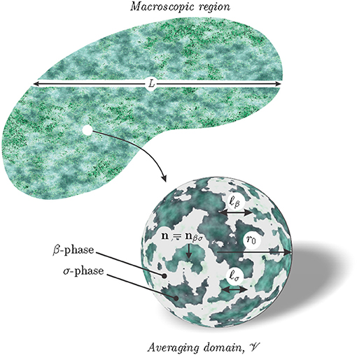
Figure 1. Schematic representation of a porous medium system including the characteristic lengths at the microscale (ℓ_β in the β-phase and ℓ_σ in the σ-phase), and at the macroscale (L) as well as the averaging domain of size r₀.

Here, ${D}$ is the molecular diffusivity of species A in the β-phase, c is the pore-scale molar concentration of species A, and v is the fluid velocity, which satisfies the total mass conservation and Stokes equations

$\begin{array}{ll}\nabla ·\text{v}=0,\text{\hspace{1em}in the }\beta \text{-phase},& (\mathrm{1b})\end{array}$

$\begin{array}{ll}0=-\nabla p+\mu \nabla ·\left(\nabla \text{v}+{(\nabla \text{v})}^T\right),\text{\hspace{1em}in the }\beta \text{-phase}.& (\mathrm{1c})\end{array}$

In the above equation, p is the pore-scale fluid pressure, μ is the dynamic fluid viscosity, assumed constant, and the body forces due to gravity may be included in the pressure gradient term. Moreover, the term ∇·(∇v)^T = ∇(∇·v) was kept for convenience of the developments that follow, although it does not bring any contribution in the pore-scale momentum balance due to the assumption of incompressible flow. Since the solid surface has been assumed to be impermeable to mass transfer, it is reasonable to impose the following interfacial boundary condition

$\begin{array}{ll}-\text{n}·{D}\nabla c=0,\text{\hspace{1em}at }{{A}}_{\beta \sigma }.& (\mathrm{1d})\end{array}$

Here, n = n_βσ is the unit normal vector directed from the fluid to the solid phase as shown in Figure 1. The tangential component of the fluid velocity vector at the interface can be expressed as the superposition of a first order viscous slip boundary condition (Einzel et al., 1990; Lauga et al., 2007) and a diffusive slip condition (Kramers and Kistemaker, 1943; Altevogt et al., 2003a; Moyne et al., 2020), assuming isothermal conditions for the binary mixture in which species A is sufficiently diluted in order for Fick's law to be applicable. In addition, the gas molecules are conceived as spheres experiencing both specular and diffuse wall collisions. The resulting expression for the boundary condition can be written as follows

$\begin{array}{ll}\text{v}=-\xi \lambda \text{n}·\left(\nabla \text{v}+\nabla {\text{v}}^T\right)·(\text{I}-\text{n}\text{n})+\frac{{D}\nabla c}{c+\alpha }·(\text{I}-\text{n}\text{n}),\text{\hspace{1em}at }{{A}}_{\beta \sigma }.& (1e)\end{array}$

In this expression, I is the identity tensor, ξ = (2 − σ_v)/σ_v (σ_v being the tangential momentum accommodation coefficient representing the fraction of particles experiencing diffuse reflection at ${{A}}_{\beta \sigma }$), λ is the mean free path and α is a coefficient given by

$\begin{array}{ll}\alpha =\frac{\rho }{\sqrt{M_A{M}_B}-M_A}.& (\mathrm{1f})\end{array}$

In this relationship, ρ is the fluid density, which is assumed constant, while M_A and M_B are, respectively, the molar mass of species A and of the solvent B. The first term on the right hand side of Equation (1e) accounts for Knudsen effects whereas the second term is due to ordinary diffusion and results from the existence of a concentration gradient in the tangential direction at the solid-fluid interface. It should be noted that the importance of the diffusive slip effect is subject to the value of α. In particular, it is expected to become more significant as the molar mass difference between the solvent and the solute is more pronounced.

The microscale model is completed by the initial condition for c and the boundary conditions at the entrances and exits of the macroscopic domain for the concentration and the pressure or the velocity. However, this information is not required for the derivation of the upscaled model that follows and it is not reported here for the sake of brevity in presentation.

In classical passive dispersion problems, for which there is no impact of the species transport on momentum transport, upscaling of the governing equations for the two processes can be carried out independently from each other (see, for example Chapters 3 and 4 in Whitaker, 1999). In such circumstances, the macroscopic model for momentum transport is usually considered as part of the background knowledge for the development of the macroscopic species transport model (see for instance Valdés-Parada et al., 2019). Here, however, both processes are intimately coupled since the concentration field retroactively impacts the velocity field as can be inferred from the slip boundary condition expressed in Equation (1e). As a result, the derivation of the macroscopic model proposed below requires that the upscaling procedure includes the complete set of equations reported above. In this work, the volume averaging method (Whitaker, 1999) is used to derive the upscaled total and species mass transport equations and, with this in mind, the basic elements of this method are summarized in the next paragraphs. However, for momentum transport a modified version of this method is used, which is consistent with the adjoint homogenization technique proposed by Bottaro (2019).

3. Essentials of the Volume Averaging Method

In order to carry out the upscaling process, it is necessary to define an averaging domain ${V}$, of norm V, that contains both solid and fluid phases such as the one sketched in Figure 1. In order for this averaging domain to be representative, its characteristic size r₀ must be much larger than the largest pore-scale characteristic size [say ℓ_p = max(ℓ_β, ℓ_σ)] and, at the same time, it must be much smaller than the smallest characteristic size associated to the macroscale, L. This is

$\begin{array}{ll}{\ell }_p\ll r_0\ll L.& (2)\end{array}$

On this averaging domain, the superficial and intrinsic averaging operators are respectively defined as (Whitaker, 1999)

$\begin{array}{ll}\langle \psi \rangle =\frac{1}{V}{\displaystyle \underset{{{V}}_{\beta }}{\int }}\psi dV,& (\mathrm{3a})\end{array}$

$\begin{array}{ll}{\langle \psi \rangle }^{\beta }=\frac{1}{V_{\beta }}{\displaystyle \underset{{{V}}_{\beta }}{\int }}\psi dV,& (\mathrm{3b})\end{array}$

with ψ being a piece-wise smooth function defined in the β-phase. These two averaging operators are related by

$\begin{array}{ll}\langle \psi \rangle =\epsilon {\langle \psi \rangle }^{\beta },& (\mathrm{3c})\end{array}$

where ε ≡ V_β/V is the volume fraction of the fluid phase contained in the averaging domain and, in this case, it corresponds to the porosity. The derivations that follow are constrained to the homogeneous regions of the system, i.e., to the portions of the porous medium located sufficiently far from the macroscopic boundaries where average properties (such as ε) can be treated as constants.

Furthermore, in order to interchange spatial differentiation and integration, the spatial averaging theorem, given by (see, for example, Howes and Whitaker, 1985)

$\begin{array}{ll}\langle \nabla \psi \rangle =\nabla \langle \psi \rangle +\frac{1}{V}{\displaystyle \underset{{{A}}_{\beta \sigma }}{\int }}\text{n}\psi dA,& (\mathrm{4a})\end{array}$

is employed. The use of this theorem requires average quantities to be continuously differentiable, as explained in this reference. Using the relationship given in Equation (3c) and taking into account the assumption that ε can be treated as a constant, the following alternative form, referred to as the modified averaging theorem in the rest of the developments, may also be used

$\begin{array}{ll}{\langle \nabla \psi \rangle }^{\beta }=\nabla {\langle \psi \rangle }^{\beta }+\frac{1}{V_{\beta }}{\displaystyle \underset{{{A}}_{\beta \sigma }}{\int }}\text{n}\psi dA.& (\mathrm{4b})\end{array}$

In most applications of the volume averaging method, it is necessary to express pore-scale quantities in terms of their intrinsic averages and spatial deviations, $\tilde{\psi }$, as proposed by Gray (1975),

$\begin{array}{ll}\psi ={\langle \psi \rangle }^{\beta }+\tilde{\psi },& (5)\end{array}$

and such a decomposition will be employed in the following. It should be noted that, on the basis of the constraint given in (2), averaged properties can be regarded as constants within the integration domain. A direct corollary of this is the following average constraint for the deviations fields

$\begin{array}{ll}{\langle \tilde{\psi }\rangle }^{\beta }=0.& (6)\end{array}$

With these elements at hand, the derivation of the macroscopic equations can be carried out and this is presented in the section that follows.

4. Upscaling

4.1. Mass Conservation Equation of Species A

Application of the intrinsic averaging operator to Equation (1a) leads to

$\begin{array}{ll}\frac{\partial {\langle c\rangle }^{\beta }}{\partial t}+\nabla ·{\langle c\text{v}\rangle }^{\beta }=\nabla ·({D}{\langle \nabla c\rangle }^{\beta }).& (7)\end{array}$

To obtain the above result, the modified spatial averaging theorem was employed and the interfacial boundary conditions were taken into account together with the assumption that the porous medium structure is rigid and homogeneous. On the basis of the latter assumption, and because the averaging domain is time independent, it follows that ${\langle \frac{\partial c}{\partial t}\rangle }^{\beta }=\frac{\partial {\langle c\rangle }^{\beta }}{\partial t}$. In addition, it was also assumed that ${D}$ can be treated as a constant within the averaging domain.

To further develop the convective term, the spatial decomposition given in Equation (5) (for ψ = c) can be substituted, and this yields

$\begin{array}{ll}\nabla ·{\langle c\text{v}\rangle }^{\beta }=\nabla ·\left({\langle c\rangle }^{\beta }{\langle \text{v}\rangle }^{\beta }\right)+\nabla ·{\langle \tilde{c}\text{v}\rangle }^{\beta }.& (8)\end{array}$

In addition, a second application of the modified averaging theorem, together with the concentration decomposition, allow expressing the diffusive term as follows

$\begin{array}{ll}\nabla ·\left({D}{\langle \nabla c\rangle }^{\beta }\right)=\nabla ·\left[{D}\left(\nabla {\langle c\rangle }^{\beta }+\frac{1}{V_{\beta }}{\displaystyle \underset{{{A}}_{\beta \sigma }}{\int }}\text{n}\tilde{c}dA\right)\right].& (9)\end{array}$

Here, 〈c〉^β was regarded as constant within the integration domain. This is supported by the combination of Equations (5) and (6), together with the separation of length scales given in (2). In addition, the assumption of spatial homogeneity was used, i.e., $\nabla \epsilon =-\frac{1}{V}{\int }_{{{A}}_{\beta \sigma }}\text{n}dA=\mathbf{\text{0}}$. Substitution of Equations (8) and (9) into Equation (7) leads to

$\begin{array}{l}\frac{\partial {\langle c\rangle }^{\beta }}{\partial t}+\nabla ·\left({\langle c\rangle }^{\beta }{\langle \text{v}\rangle }^{\beta }\right)+\nabla ·{\langle \tilde{c}\text{v}\rangle }^{\beta }\\ =\nabla ·\left[{D}\left(\nabla {\langle c\rangle }^{\beta }+\frac{1}{V_{\beta }}{\displaystyle \underset{{{A}}_{\beta \sigma }}{\int }}\text{n}\tilde{c}dA\right)\right].& (10)\end{array}$

The above expression is the unclosed average equation for species A mass transport. The reason for this terminology is due to the fact that it contains integral terms (i.e., filters of information from the pore-scale) involving spatial deviations variables. In order to make further progress, it is necessary to have information about how the concentration deviations, $\tilde{c}$, are related to average fields and this step will be addressed later. At this point, it is pertinent to perform the averaging of the total mass equation.

4.2. Total Mass Conservation Equation

Applying the superficial averaging operator to Equation (1b) and using the averaging theorem in its divergence form, together with the fact that the velocity is tangential at the solid-fluid interface, leads to

$\begin{array}{ll}\nabla ·\langle \text{v}\rangle =0.& (\mathrm{11a})\end{array}$

Using the relationship given in Equation (3c), the above equation can be written in terms of the intrinsic average of the fluid velocity

$\begin{array}{ll}\nabla ·{\langle \text{v}\rangle }^{\beta }=0.& (\mathrm{11b})\end{array}$

Here, again, the assumption of spatial homogeneity, i.e., a constant porosity, was considered. Both versions of the macroscopic total mass conservation equation listed above are closed and do not require further derivations. As a final remark, it is worth noting that Equation (11b) is recovered by making the sum of Equation (10) for all the chemical species involved in the mixture.

5. Closure

As already mentioned, expressions of the deviations in terms of average quantities, a process usually referred to as closure, is necessary in order to complete the upscaled model. This is carried out by considering the following steps: (1) Derivation of the governing equations for the deviations as well as the corresponding boundary conditions; (2) Imposition of some reasonable simplifications in order to reduce the complexity of the resulting problem and (3) Formal solution of the problem in order to find the relationships between deviations and average quantities. Usually a set of length-scale constraints and assumptions, which can be regarded as scaling postulates, as suggested by Wood and Valdés-Parada (2013), are involved in step 2.

5.1. Conservation Equation for Species A

In order to derive the governing equation for $\tilde{c}$, Equation (5) suggests subtracting Equation (10) from the mass balance equation for species A at the pore scale, i.e., Equation (1a). The result is

$\begin{array}{l}\frac{\partial \tilde{c}}{\partial t}+\nabla ·({\langle c\rangle }^{\beta }\tilde{\text{v}})+\nabla ·(\tilde{c}\text{v})-\nabla ·{\langle \tilde{c}\text{v}\rangle }^{\beta }\\ =\nabla ·({D}\nabla \tilde{c})-\nabla ·\left(\frac{{D}}{V_{\beta }}{\displaystyle \underset{{{A}}_{\beta \sigma }}{\int }}\text{n}\tilde{c}dA\right),\text{\hspace{1em}in the }\beta \text{-phase}.& (12)\end{array}$

With the intention of simplifying this equation, it may be noticed, on the one hand, that the order of magnitude estimates for the non-local diffusion and convection terms can be expressed as

$\begin{array}{lll}\nabla ·\left(\frac{{D}}{V_{\beta }}{\displaystyle \underset{{{A}}_{\beta \sigma }}{\int }}\text{n}\tilde{c}dA\right)=& \text{O}\left(\frac{{D}\tilde{c}}{L}\frac{A_{\beta \sigma }}{V_{\beta }}\right),& (\mathrm{13a})\end{array}$

$\begin{array}{ll}\nabla ·{\langle \tilde{c}\text{v}\rangle }^{\beta }=\text{O}\left(\frac{\tilde{c}v}{L}\right).& (\mathrm{13b})\end{array}$

Here, A_βσ and v represent the order of magnitude estimates of the measure of ${A}$_βσ and v, respectively. On the other hand, the estimates for the local diffusive and convective terms are given by

$\begin{array}{lll}\nabla ·({D}\nabla \tilde{c})& =\text{O}\left(\frac{{D}\tilde{c}}{{\ell }_{\beta }^2}\right),& (\mathrm{14a})\end{array}$

$\begin{array}{lll}\nabla ·(\tilde{c}\text{v})& =\text{O}\left(\frac{\tilde{c}v}{{\ell }_{\beta }}\right).& (\mathrm{14b})\end{array}$

Therefore, on the basis of the constraints ℓ_β ≪ L and $\frac{A_{\beta \sigma }{\ell }_{\beta }^2}{V_{\beta }L}\ll 1$, it is reasonable to assume that

$\begin{array}{ll}\nabla ·\left(\frac{{D}}{V_{\beta }}{\displaystyle \underset{{{A}}_{\beta \sigma }}{\int }}\text{n}\tilde{c}dA\right)\ll \nabla ·({D}\nabla \tilde{c}),& (\mathrm{15a})\end{array}$

$\begin{array}{ll}\nabla ·{\langle \tilde{c}\text{v}\rangle }^{\beta }\ll \nabla ·(\tilde{c}\text{v}).& (\mathrm{15b})\end{array}$

Hence, Equation (12) may be simplified to

$\begin{array}{ll}\frac{\partial \tilde{c}}{\partial t}+\tilde{\text{v}}·\nabla {\langle c\rangle }^{\beta }+\nabla ·(\tilde{c}\text{v})=\nabla ·({D}\nabla \tilde{c}),\text{\hspace{1em}in the }\beta \text{-phase}.& (16)\end{array}$

It should be noted that, in order to arrive at this last expression, the total mass conservation Equations (1b) and (11b) were employed.

At this point, it is pertinent to estimate the order of magnitude of the accumulation term as follows

$\begin{array}{ll}\frac{\partial \tilde{c}}{\partial t}=\text{O}\left(\frac{\tilde{c}}{t^{*}}\right),& (17)\end{array}$

where t^* represents the time scale at which $\tilde{c}$ experiences significant variations. Moreover, from Equations (14), the combined order of magnitude estimates of the local diffusive and convective terms can be shown to be $\text{O}\left(\tilde{c}{D}(1+Pe)/{\ell }_{\beta }^2\right)$ where the Péclet number, Pe, is defined as

$\begin{array}{ll}Pe=\frac{v{\ell }_{\beta }}{{D}}.& (18)\end{array}$

Therefore, it is deduced that, when the following time-scale constraint is met

$\begin{array}{ll}\frac{{\ell }_{\beta }^2}{{D}(1+Pe)}\ll t^{*},& (19)\end{array}$

Equation (16) may be considered to be quasi-steady, i.e.,

$\begin{array}{ll}\tilde{\text{v}}·\nabla {\langle c\rangle }^{\beta }+\text{v}·\nabla \tilde{c}=\nabla ·({D}\nabla \tilde{c}),\text{\hspace{1em}in the }\beta \text{-phase}.& (20)\end{array}$

This temporal constraint is retained in the remainder of the analysis.

5.2. Momentum Transport Equation

The equation for total mass conservation at the pore-scale given in Equation (1b) is still useful for the closure problem solution in its current form. Nevertheless, it is convenient to spatially decompose the pressure, using Equation (5) with ψ = p, in the Stokes equation to obtain

$\begin{array}{ll}0=-\nabla \tilde{p}+\mu \nabla ·\left(\nabla \text{v}+{(\nabla \text{v})}^T\right)-\nabla {\langle p\rangle }^{\beta },\text{\hspace{1em}in the }\beta \text{-phase}.& (21)\end{array}$

For the derivations that follow it is not necessary to apply the spatial decomposition for the velocity and therefore no further developments are required in the above equation.

5.3. Interfacial Boundary Conditions

Substituting the spatial decomposition for the species concentration into Equation (1d), leads to

$\begin{array}{ll}-\text{n}·\nabla \tilde{c}=\text{n}·\nabla {\langle c\rangle }^{\beta },\text{\hspace{1em}at }{{A}}_{\beta \sigma }.& (22)\end{array}$

Before proceeding with the slip condition for the velocity, an order of magnitude analysis can now be performed on this result in order to obtain the following estimate for $\tilde{c}$

$\begin{array}{ll}\tilde{c}=\text{O}\left(\frac{{\ell }_{\beta }}{L}{\langle c\rangle }^{\beta }\right).& (23)\end{array}$

According to the length-scale constraint expressed as ℓ_β ≪ L, this leads to the following assumption

$\begin{array}{ll}\tilde{c}\ll {\langle c\rangle }^{\beta }.& (24)\end{array}$

Directing now the attention to the velocity slip boundary condition, let the pore-scale concentration be decomposed into its average and deviations in Equation (1e) in order to obtain

$\begin{array}{r}\text{v}=-\xi \lambda \text{n}·\left(\nabla \text{v}+\nabla {\text{v}}^T\right)·(\text{I}-\text{n}\text{n})+\frac{{D}\nabla \tilde{c}}{{\langle c\rangle }^{\beta }+\alpha }·(\text{I}-\text{n}\text{n})\\ +\frac{{D}\nabla {\langle c\rangle }^{\beta }}{{\langle c\rangle }^{\beta }+\alpha }·(\text{I}-\text{n}\text{n}),\text{\hspace{1em}at }{{A}}_{\beta \sigma }.& (25)\end{array}$

Note that the assumption given in (24) was used in the terms at the denominator of this last expression. The purpose of such an approximation is to maintain a linear problem for the concentration deviations as it is commonly done in applications of the volume averaging method (see, for example Wood and Whitaker, 1998; Valdés-Parada et al., 2009).

5.4. Local Closure Problem

Since the determination of the deviations fields in the entire macroscopic domain would be, at least, as complicated as solving the original pore-scale equations everywhere, the interest is not to carry out a solution of the closure problem over the entire macroscopic system. Instead, it is more convenient to solve the closure problem within a representative solution domain such as the one sketched in Figure 2, which corresponds to a unit cell of the porous medium assimilated to a periodic structure. In this domain, Taylor series expansions for all the average quantities involved in the closure problems can be performed about the centroid of the unit cell located by the position vector denoted by x. On the basis of the separation of length scales, r₀ ≪ L, these series can be truncated at the zeroth order as explained in Chapter 1 of Whitaker (1999). Under these conditions, the local closure problem takes the following form

Total mass transport

$\begin{array}{ll}\nabla ·\text{v}=0,\text{\hspace{1em}in the }\beta \text{-phase}.& (\mathrm{26a})\end{array}$

Total momentum transport

$\begin{array}{ll}0=-\frac{1}{\mu }\nabla \tilde{p}+\nabla ·\left(\nabla \text{v}+{(\nabla \text{v})}^T\right){\displaystyle \underset{source}{{\displaystyle \underbrace{-\frac{1}{\mu }\nabla {\langle p\rangle }^{\beta }{|}_{\text{x}}}}}},\text{\hspace{1em}in the }\beta \text{-phase}.& (\mathrm{26b})\end{array}$

Species A mass transport

$\begin{array}{ll}\tilde{\text{v}}·{\displaystyle \underset{source}{{\displaystyle \underbrace{\text{f}{|}_{\text{x}}}}}}+\text{v}·\nabla \tilde{\chi }=\nabla ·({D}\nabla \tilde{\chi }),\text{\hspace{1em}in the }\beta \text{-phase}.& (\mathrm{26c})\end{array}$

Interfacial boundary conditions

$\begin{array}{ll}-\text{n}·\nabla \tilde{\chi }=\text{n}·{\displaystyle \underset{source}{{\displaystyle \underbrace{\text{f}{|}_{\text{x}}}}}},\text{\hspace{1em}at }{{A}}_{\beta \sigma }.& (\mathrm{26d})\end{array}$

$\begin{array}{r}\text{v}=-\xi \lambda \text{n}·\left(\nabla \text{v}+\nabla {\text{v}}^T\right)·(\text{I}-\text{n}\text{n})+{D}\nabla \tilde{\chi }·(\text{I}-\text{n}\text{n})\\ +{D}{\displaystyle \underset{source}{{\displaystyle \underbrace{\text{f}{|}_{\text{x}}}}}}·(\text{I}-\text{n}\text{n}),\text{\hspace{1em}at }{{A}}_{\beta \sigma }.& (26e)\end{array}$

Periodicity

$\begin{array}{ll}\text{v}(\text{r}+{\text{l}}_i)=\text{v}(\text{r});\tilde{p}(\text{r}+{\text{l}}_i)=\tilde{p}(\text{r});\tilde{\chi }(\text{r}+{\text{l}}_i)=\tilde{\chi }(\text{r}),i=1,2,3.& (\mathrm{26f})\end{array}$

FIGURE 2

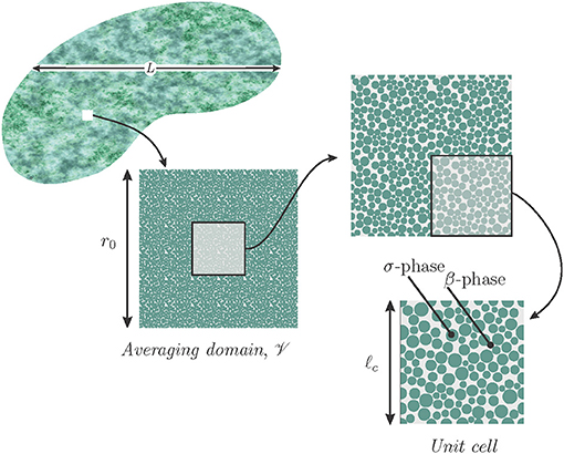
Figure 2. Sketch of a two-dimensional periodic unit cell, of side length ℓ_c, for solving the closure problem.

Average constraints

$\begin{array}{ll}{\langle \tilde{p}\rangle }^{\beta }=0;{\langle \tilde{\chi }\rangle }^{\beta }=0.& (\mathrm{26g})\end{array}$

For the sake of brevity in writing, the following definitions were used in Equations (26c)–(26g)

$\begin{array}{ll}\tilde{\chi }=\frac{\tilde{c}}{{\langle c\rangle }^{\beta }{|}_{\text{x}}+\alpha };\text{f}{|}_{\text{x}}=\frac{\nabla {\langle c\rangle }^{\beta }{|}_{\text{x}}}{{\langle c\rangle }^{\beta }{|}_{\text{x}}+\alpha }.& (27)\end{array}$

In addition, the fact that ${\langle c\rangle }^{\beta }{|}_{\text{x}}$ can be treated as a constant within the unit cell was employed. With the consideration of locality for the closure problem, it becomes clear that the velocity is a variable that does not need to be decomposed according to Equation (5) since v can be considered as a periodic field at the level of the unit cell.

Note that, due to the convective term in Equation (26c), the problem is non-linear and hence a formal solution is not achievable, in general. To overcome this issue, the velocity in this term might be regarded as a known field, an assumption that is consistent with previous studies of upscaling in porous media involving nonlinear mechanisms (see, for instance, Bottaro, 2019; Lasseux et al., 2019). This allows linearizing the closure problem and integral equations formulations based on Green's functions may then be used, as suggested by Wood and Valdés-Parada (2013) or Bottaro (2019) while employing the adjoint homogenization method, to obtain the following formal solution for v, $\tilde{p}$ and $\tilde{\chi }$ as linear functions of the sources identified in Equation (26)

$\begin{array}{ll}\text{v}=-\frac{\text{A}}{\mu }·\nabla {\langle p\rangle }^{\beta }+\text{C}·\text{f},& (\mathrm{28a})\end{array}$

$\begin{array}{ll}\tilde{p}=-\text{a}·\nabla {\langle p\rangle }^{\beta }+\mu \text{c}·\text{f},& (\mathrm{28b})\end{array}$

$\begin{array}{ll}\tilde{\chi }=-\frac{\text{d}}{\mu }·\nabla {\langle p\rangle }^{\beta }+\text{e}·\text{f}.& (\mathrm{28c})\end{array}$

In these expressions, the closure variables A, C, a, c, d and e are integrals of the corresponding Green's functions. In this way, the closure variables may be interpreted as mapping functions of the sources onto v, $\tilde{p}$ and $\tilde{\chi }$, respectively.

Substitution of Equation (28) into Equation (26) and splitting them according to the source gives rise to the following boundary-value problems in terms of the closure variables

Problem-I (source $-\frac{1}{\mu }\nabla {\langle p\rangle }^{\beta }$)

$\begin{array}{ll}\nabla ·\text{A}=0,\text{\hspace{1em}in the }\beta \text{-phase},& (\mathrm{29a})\end{array}$

$\begin{array}{ll}0=-\nabla \text{a}+\nabla ·\left(\nabla \text{A}+{(\nabla \text{A})}^{T1}\right)+\text{I},\text{\hspace{1em}in the }\beta \text{-phase},& (\mathrm{29b})\end{array}$

$\begin{array}{ll}\text{v}·\nabla \text{d}=\nabla ·({D}\nabla \text{d}),\text{\hspace{1em}in the }\beta \text{-phase},& (\mathrm{29c})\end{array}$

$\begin{array}{ll}-\text{n}·\nabla \text{d}=0,\text{\hspace{1em}at }{{A}}_{\beta \sigma },& (\mathrm{29d})\end{array}$

$\begin{array}{ll}\text{A}=-\xi \lambda \text{n}·\left(\nabla \text{A}+{(\nabla \text{A})}^{T1}\right)·(\text{I}-\text{n}\text{n})+{D}\nabla \text{d}·(\text{I}-\text{n}\text{n}),\text{\hspace{1em}at }{{A}}_{\beta \sigma },& (29e)\end{array}$

$\begin{array}{ll}\psi (\text{r}+{\text{l}}_i)=\psi (\text{r}),i=1,2,3;\psi =\text{A},\text{a},\text{d},& (\mathrm{29f})\end{array}$

$\begin{array}{ll}{\langle \text{a}\rangle }^{\beta }=0;{\langle \text{d}\rangle }^{\beta }=0.& (\mathrm{29g})\end{array}$

Problem-II (source f)

$\begin{array}{ll}\nabla ·\text{C}=0,\text{\hspace{1em}in the }\beta \text{-phase},& (\mathrm{30a})\end{array}$

$\begin{array}{ll}0=-\nabla \text{c}+\nabla ·\left(\nabla \text{C}+{(\nabla \text{C})}^{T1}\right),\text{\hspace{1em}in the }\beta \text{-phase},& (\mathrm{30b})\end{array}$

$\begin{array}{ll}\tilde{\text{v}}+\text{v}·\nabla \text{e}=\nabla ·({D}\nabla \text{e}),\text{\hspace{1em}in the }\beta \text{-phase},& (\mathrm{30c})\end{array}$

$\begin{array}{ll}-\text{n}·\nabla \text{e}=\text{n},\text{\hspace{1em}at }{{A}}_{\beta \sigma },& (\mathrm{30d})\end{array}$

$\begin{array}{l}\text{C}=-\xi \lambda \text{n}·\left(\nabla \text{C}+{(\nabla \text{C})}^{T1}\right)·(\text{I}-\text{n}\text{n})+{D}\nabla \text{e}·(\text{I}-\text{n}\text{n})\\ +{D}(\text{I}-\text{n}\text{n}),\text{\hspace{1em}at }{{A}}_{\beta \sigma },& (30e)\end{array}$

$\begin{array}{ll}\psi (\text{r}+{\text{l}}_i)=\psi (\text{r}),i=1,2,3;\psi =\text{c},\text{C},\text{e},& (\mathrm{30f})\end{array}$

$\begin{array}{ll}{\langle \text{c}\rangle }^{\beta }=0;{\langle \text{e}\rangle }^{\beta }=0.& (\mathrm{30g})\end{array}$

In the above equations, the superscript T1 was used to denote the transpose, which, for a third order tensor, κ, permutes the first and second indices, i.e., ${\kappa }_{ijk}^{T1}={\kappa }_{jik}$.

The two closure problems I and II are coupled both between themselves and also with the macroscale model solution due to the convective terms in Equations (29c) and (30c). This becomes clear when, in these two last equations, the representation given in Equation (28a) is used to express $\tilde{\text{v}}$ and v in terms of ∇〈p〉^β and f. This issue is often encountered while upscaling non-linear processes (see, for instance, Valdés-Parada et al., 2009; Airiau and Bottaro, 2020) and it will be addressed later in section 6.3. At this point, it is pertinent to derive the closed form of the upscaled model.

6. Closed Model

Now that expressions relating v, $\tilde{p}$ and $\tilde{\chi }$ to average quantities are available, it is of interest to return to the average equations and express them in a closed manner. For total mass transport, the closed equation is given by either one of Equation (11).

6.1. Closed Macroscopic Momentum Equation

For momentum transport, the corresponding equation results from applying the superficial averaging operator to Equation (28a). This leads to

$\begin{array}{ll}\langle \text{v}\rangle =-\frac{{\text{K}}_s}{\mu }·\nabla {\langle p\rangle }^{\beta }+{\text{D}}_c·\frac{\nabla {\langle c\rangle }^{\beta }}{{\langle c\rangle }^{\beta }+\alpha },& (31)\end{array}$

where the following nomenclature was used

$\begin{array}{ll}{\text{K}}_s=\langle \text{A}\rangle ;{\text{D}}_c=\langle \text{C}\rangle .& (32)\end{array}$

Here, K_s is an apparent permeability tensor that differs from the intrinsic one as it is affected by both the diffusive and viscous slip effects. This tensor reduces to the intrinsic permeability tensor under no-slip conditions. In addition, D_c is a dispersion tensor, which, for conditions such that Knudsen effects can be disregarded, reduces to the macroscopic slip conductivity introduced by Altevogt et al. (2003a). It should be emphasized that the two effective medium coefficients appearing in Equation (31) depend on the Péclet number defined in Equation (18) and the Knudsen number, Kn, given by

$\begin{array}{ll}Kn=\lambda /{\ell }_{\beta }.& (33)\end{array}$

The specific nature of this dependency should be extensively studied but the details of this dependency are, however, beyond the scope of this work. Nevertheless, an analysis is presented in section 7 in terms of the Péclet number, allowing to retrieve some transport regimes reported in the literature. The physical meaning of the two terms appearing on the right-hand side of Equation (31) can be understood as follows. The first term is related to momentum transport due to the macroscopic pressure gradient. The second term can be regarded as a correction to momentum transport induced by both slip effects.

6.2. Closed Macroscopic Species Transport Equation

The remaining equation to be closed is the one governing transport of species A. To progress toward this macroscopic equation, the definitions given in Equation (27) can be introduced back into Equation (28c) in order to express the latter as

$\begin{array}{ll}\tilde{c}=-({\langle c\rangle }^{\beta }+\alpha )\frac{\text{d}}{\mu }·\nabla {\langle p\rangle }^{\beta }+\text{e}·\nabla {\langle c\rangle }^{\beta }.& (34)\end{array}$

Substituting this result into Equation (10) yields

$\begin{array}{ll}{\displaystyle \underset{\text{mass accumulation}}{{\displaystyle \underbrace{\frac{\partial {\langle c\rangle }^{\beta }}{\partial t}}}}}+{\displaystyle \underset{\text{convective transport}}{{\displaystyle \underbrace{\nabla ·\left({\langle c\rangle }^{\beta }{\langle \text{v}\rangle }^{\beta }\right)}}}}& +{\displaystyle \underset{\text{slip correction to convective transport}}{{\displaystyle \underbrace{\nabla ·\left[({\langle c\rangle }^{\beta }+\alpha )\frac{\text{R}}{\mu }·\nabla {\langle p\rangle }^{\beta }\right]}}}}\\ ={\displaystyle \underset{\genfrac{}{}{0ex}{}{\text{mass dispersion including}}{\text{slip effects}}}{{\displaystyle \underbrace{\nabla ·\left[{\text{D}}_s·\nabla {\langle c\rangle }^{\beta }\right]}}}},& (35)\end{array}$

where the physical meaning of each term was identified and the following effective-medium coefficients were introduced

$\begin{array}{ll}\text{R}=-{\langle \tilde{\text{v}}\text{d}\rangle }^{\beta }+\frac{{D}}{V_{\beta }}{\displaystyle \underset{{{A}}_{\beta \sigma }}{\int }}\text{n}\text{d}dA,& (\mathrm{36a})\end{array}$

$\begin{array}{ll}{\text{D}}_s={D}\left(\text{I}+\frac{1}{V_{\beta }}{\displaystyle \underset{{{A}}_{\beta \sigma }}{\int }}\text{n}\text{e}dA-{{D}}^{-1}{\langle \tilde{\text{v}}\text{e}\rangle }^{\beta }\right).& (\mathrm{36b})\end{array}$

Equation (35) differs from the typical convection-dispersion equation as it contains a slip correction to convective transport and it requires the computation of two effective-medium coefficients. The second order tensor, R, has the units of permeability and the product $\frac{\mathbf{\text{R}}}{\mu }·\nabla {\langle p\rangle }^{\beta }$ may be interpreted as a velocity vector that corrects 〈v〉^β in order to account for slip effects. In addition, the dispersion tensor, D_s, given in Equation (36b), is defined in a similar manner as the total dispersion tensor encountered in passive dispersion in porous media (see Chapter 3 in Whitaker, 1999). The main difference with this case lies in the fact that the closure variable, e, depends on both Knudsen and diffusive slip effects as it is evidenced in Problem-II (see Equations 30).

6.3. Summary of the Closed Average Model

The closed average model consists of the effective-medium equations given in Equations (11a) or (11b) (total mass conservation), Equation (31) (momentum transport) and Equation (35) (species A mass transport). These three balance equations may be combined to provide an equivalent alternative form of the average model made of two equations on ∇〈p〉^β and 〈c〉^β, respectively. Introducing the expression of the average velocity given in the macroscopic momentum Equation (31) into the averaged total mass conservation Equation (11a) yields

$\begin{array}{ll}\nabla ·\left(\frac{{\text{K}}_s}{\mu }·\nabla {\langle p\rangle }^{\beta }-\frac{{\text{D}}_c}{{\langle c\rangle }^{\beta }+\alpha }·\nabla {\langle c\rangle }^{\beta }\right)=0.& (37)\end{array}$

Similarly, replacing the average velocity in the macroscopic equation for species A mass transport by the modified Darcy Equation (31), and rearranging, leads to

$\begin{array}{l}\epsilon \frac{\partial {\langle c\rangle }^{\beta }}{\partial t}+\frac{1}{\mu }\nabla ·\left[(\epsilon ({\langle c\rangle }^{\beta }+\alpha )\text{R}-{\langle c\rangle }^{\beta }{\text{K}}_s)·\nabla {\langle p\rangle }^{\beta }\right]\\ =\nabla ·\left[\left(\epsilon {\text{D}}_s-\frac{{\langle c\rangle }^{\beta }{\text{D}}_c}{{\langle c\rangle }^{\beta }+\alpha }\right)·\nabla {\langle c\rangle }^{\beta }\right].& (38)\end{array}$

These two equations clearly show the non-linear coupling between the macroscopic pressure gradient and macroscopic concentration. Once the solutions on ∇〈p〉^β and 〈c〉^β are achieved, subject to macroscopic boundary and initial conditions, they can be further employed to reconstruct the local velocity field using Equation (28a) over the unit cell. This is necessary to solve the two closure problems I and II yielding the four effective coefficients. The successive resolution of the macroscopic model and closure problems should be iteratively repeated until convergence is reached. Ultimately, the converged fields of ∇〈p〉^β and 〈c〉^β can be substituted in Equation (31) to predict the macroscale velocity.

In the following paragraphs, particular forms of the upscaled model are investigated. This analysis is of interest since it shows that the upscaled model derived here is general enough as it allows retrieving the resulting models reported for particular flow and transport conditions. These submodels have been thoroughly analyzed and validated and they hence serve as an indirect validation of the upscaled model derived here.

7. Particular Cases of the Upscaled Model

The upscaled model derived in the previous paragraphs is general in the sense that it is not constrained to a particular range of Péclet or Knudsen numbers values, the latter being non-zero and, at most, ~0.1 to be compliant with the slip convective regime. However, it is instructive to analyze how the structure of the model is modified for specific flow and transport conditions (more specifically regarding the momentum transport and species A mass transport equations, the total mass conservation equation remaining unaltered). In essence, the regimes are related to the relative importance of diffusive and convective effects. In the absence of diffusive slip effects, the crossover between the convective and diffusive regimes is characterized by Pe = 1 as can be easily inferred from the transport equation for $\tilde{c}$ (see Equation 20). However, a close attention to the right-hand side of the slip boundary condition given in Equation (25), once multiplied by ℓ_β/${D}$, indicates that the term related to Knudsen slip is O(PeξKn) whereas the diffusive slip term is O(ℓ_β/L). As a consequence, on the basis of this interfacial boundary condition, the three regimes to be considered here are: (1) the diffusive slip regime for which Pe ≪ ℓ_β/(LξKn); (2) the slip regime containing both slip effects where Pe = O(ℓ_β/(LξKn)) and finally, (3) the Knudsen slip regime, for which Pe ≫ ℓ_β/(LξKn). In the following paragraphs, some comments about each regime are provided.

7.1. Diffusive Slip Regime $(Pe\ll \frac{{\ell }_{\beta }}{L\xi Kn})$

In this case, the physical pore-scale model for mass and momentum transport corresponds to the one studied by Altevogt et al. (2003a) under non-adsorption conditions and to the one recently reported by Moyne et al. (2020) under incompressible flow condition and transport of a single chemical species. Furthermore, the interfacial boundary conditions in closure problems I and II given in Equations (29e) and (30e) reduce to

$\begin{array}{ll}\text{A}={D}\nabla \text{d}·(\text{I}-\text{n}\text{n}),\text{\hspace{1em}at }{{A}}_{\beta \sigma },& (39)\end{array}$

$\begin{array}{ll}\text{C}={D}\nabla \text{e}·(\text{I}-\text{n}\text{n})+{D}(\text{I}-\text{n}\text{n}),\text{\hspace{1em}at }{{A}}_{\beta \sigma }.& (40)\end{array}$

The remaining parts of the closure problems are kept unaltered, in general. Consequently, no further simplification to the upscaled model for mass and momentum transport derived here is possible. It is worth pointing out that the mathematical structure of the closure problems in this case is simpler than the one proposed by Altevogt et al. (2003a), since they are not written in an integro-differential form. Nevertheless, the formulations are equivalent.

7.2. Knudsen and Diffusive Slip Regime $(Pe=\text{O}\left(\frac{{\ell }_{\beta }}{L\xi Kn}\right))$

This regime corresponds to the general situation addressed in the previous section of the work and, to the best of our knowledge it has not been studied in the literature. Consequently, the closure problems and the upscaled model need to be solved in a coupled and iterative manner as explained above, a task that is beyond the scope of this work.

7.3. Knudsen Slip Regime $(Pe\gg \frac{{\ell }_{\beta }}{L\xi Kn})$

In this situation, Problem-I can be decoupled into the following two boundary-value problems

Problem-Ia

$\begin{array}{ll}\nabla ·\text{A}=0,\text{\hspace{1em}in the }\beta \text{-phase},& (\mathrm{41a})\end{array}$

$\begin{array}{ll}0=-\nabla \text{a}+\nabla ·\left(\nabla \text{A}+{(\nabla \text{A})}^{T1}\right)+\text{I},\text{\hspace{1em}in the }\beta \text{-phase},& (\mathrm{41b})\end{array}$

$\begin{array}{ll}\text{A}=-\xi \lambda \text{n}·\left(\nabla \text{A}+{(\nabla \text{A})}^{T1}\right)·(\text{I}-\text{n}\text{n}),\text{\hspace{1em}at }{{A}}_{\beta \sigma },& (\mathrm{41c})\end{array}$

$\begin{array}{ll}\psi (\text{r}+{\text{l}}_i)=\psi (\text{r}),i=1,2,3;\psi =\text{A},\text{a},& (\mathrm{41d})\end{array}$

$\begin{array}{ll}{\langle \text{a}\rangle }^{\beta }=0.& (41e)\end{array}$

Problem-Ib

$\begin{array}{ll}\text{v}·\nabla \text{d}=\nabla ·({D}\nabla \text{d}),\text{\hspace{1em}in the }\beta \text{-phase},& (42)\end{array}$

$\begin{array}{ll}-\text{n}·\nabla \text{d}=0,\text{\hspace{1em}at }{{A}}_{\beta \sigma },& (43)\end{array}$

$\begin{array}{ll}\text{d}(\text{r}+{\text{l}}_i)=\text{d}(\text{r}),i=1,2,3,& (44)\end{array}$

$\begin{array}{ll}{\langle \text{d}\rangle }^{\beta }=0.& (45)\end{array}$

In addition, a similar decoupling applies for Problem-II that gives rise to the following two closure problems

Problem-IIa

$\begin{array}{ll}\nabla ·\text{C}=0,\text{\hspace{1em}in the }\beta \text{-phase},& (\mathrm{46a})\end{array}$

$\begin{array}{ll}0=-\nabla \text{c}+\nabla ·\left(\nabla \text{C}+{(\nabla \text{C})}^{T1}\right),\text{\hspace{1em}in the }\beta \text{-phase},& (\mathrm{46b})\end{array}$

$\begin{array}{ll}\text{C}=-\xi \lambda \text{n}·\left(\nabla \text{C}+{(\nabla \text{C})}^{T1}\right)·(\text{I}-\text{n}\text{n}),\text{\hspace{1em}at }{{A}}_{\beta \sigma },& (\mathrm{46c})\end{array}$

$\begin{array}{ll}\psi (\text{r}+{\text{l}}_i)=\psi (\text{r}),i=1,2,3;\psi =\text{c},\text{C},& (\mathrm{46d})\end{array}$

$\begin{array}{ll}{\langle \text{c}\rangle }^{\beta }=0.& (46e)\end{array}$

Problem-IIb

$\begin{array}{ll}\tilde{\text{v}}+\text{v}·\nabla \text{e}=\nabla ·({D}\nabla \text{e}),\text{\hspace{1em}in the }\beta \text{-phase},& (\mathrm{46f})\end{array}$

$\begin{array}{ll}-\text{n}·\nabla \text{e}=\text{n},\text{\hspace{1em}at }{{A}}_{\beta \sigma },& (\mathrm{46g})\end{array}$

$\begin{array}{ll}\text{e}(\text{r}+{\text{l}}_i)=\text{e}(\text{r}),i=1,2,3,& (\mathrm{46h})\end{array}$

$\begin{array}{ll}{\langle \text{e}\rangle }^{\beta }=0.& (\mathrm{46i})\end{array}$

Note that the solution of Problem-Ib is simply d = 0 and, according to Equation (36a), this leads to R = 0. In a similar way, the solution of Problem-IIa is C = 0, thus making D_c = 0 (see the second of Equation 32). In this way, the only remaining non-zero effective-medium coefficients are the apparent permeability tensor K_s and the dispersion tensor D_s. A detailed analysis of the functionality of K_s with the geometry and the Knudsen number is available from the works by Lasseux et al. (2014) and Lasseux et al. (2016). Moreover, the disperson coefficient D_s is still given by Equation (36b) and is influenced by the Knudsen slip effects. The macroscopic mass transport equation for species A in the present situation coincides to that explored in detail in the work by Valdés-Parada et al. (2019) when the problem reported in this last reference is conceived without any heterogeneous reaction. This model is the convection-dispersion equation ant it can be written as follows

$\begin{array}{ll}\frac{\partial {\langle c\rangle }^{\beta }}{\partial t}+{\langle \text{v}\rangle }^{\beta }·\nabla {\langle c\rangle }^{\beta }=\nabla ·\left({\text{D}}_s·\nabla {\langle c\rangle }^{\beta }\right).& (47)\end{array}$

In any of the above three regimes, it is possible to encounter situations for which Pe ≪ 1. Under this constraint, a reasonable approximation for Equation (29c) is

$\begin{array}{ll}\nabla ·({D}\nabla \text{d})\simeq 0,\text{\hspace{1em}in the }\beta \text{-phase}.& (48)\end{array}$

Since d must satisfy the boundary conditions given in Equations (29d) and (29f), together with the average constraint in the second of Equation (29g), it is deduced that d ≃ 0 in this regime. The consequence of this is that, as indicated by Equation (36a), R ≃ 0. In addition, from Problem-II, under the constraint Pe ≪ 1, taking into account the estimate e = O(ℓ_β), Equation (30c) can be reasonably reduced to

$\begin{array}{ll}\nabla ·({D}\nabla \text{e})\simeq 0,\text{\hspace{1em}in the }\beta \text{-phase}.& (49)\end{array}$

This equation is subject to the boundary conditions given in Equations (30d) and (30f), which, together with the average constraint given in the second of Equation (30g), forms a problem that is decoupled from that on C and c and coincides with the closure problem for mass diffusion given in Equations (1.4–58) in Whitaker (1999). Consistently, the dispersion tensor given in Equation (36b) reduces to an effective diffusion tensor, D_eff defined as

$\begin{array}{ll}{\text{D}}_{\text{eff}}={D}\left(\text{I}+\frac{1}{V_{\beta }}{\displaystyle \underset{{{A}}_{\beta \sigma }}{\int }}\text{n}\text{e}dA\right).& (50)\end{array}$

Under these circumstances, the upscaled mass transport equation for species A given in Equation (35) reduces to

$\begin{array}{ll}\frac{\partial {\langle c\rangle }^{\beta }}{\partial t}=\nabla ·\left({\text{D}}_{\text{eff}}·\nabla {\langle c\rangle }^{\beta }\right),& (51)\end{array}$

showing, as expected, that the macroscopic species mass transport is purely diffusive when Pe ≪ 1, whatever the nature of the slip velocity boundary condition. In addition, the upscaled equation for momentum transport given in Equation (31) remains unaltered. However, when the Péclet number value is such that the interfacial and bulk transports are both purely diffusive, i.e., when Pe ≪ min (ℓ_β/(LξKn), 1), the permeability tensor K_s reduces to the intrinsic permeability tensor.

8. Conclusion

In this work, the problem of gas mixture transport in a homogeneous porous medium was addressed with the purpose of deriving an upscaled model. With this aim in mind, the pore-scale problem was formulated in the case of a binary mixture involving a passive solute diluted in a solvent that is transported by advection and diffusion. Slip flow, due to Knudsen effects, as well as diffusive slip are taken into account at the solid-fluid interface following a first-order Navier condition for momentum and a Kramers-Kistemaker condition for species transport. In addition, this interface is considered impervious to mass transfer. Assuming incompressible and isothermal flow, the total and solute species mass conservation equations, together with the momentum balance equation for the fluid mixture associated to the slip boundary condition were upscaled by means of the volume averaging method, complemented with an approach similar to that used in the adjoint homogenization method. The result is a macroscopic model including the corresponding macroscopic balance equations. The macroscopic total mass conservation equation is the classical divergence-free average velocity. The macroscopic momentum balance equation involves a Darcy term but with an apparent permeability tensor that is the intrinsic permeability corrected by both slip effects. An additional term, accounting for momentum induced by the interfacial diffusive slip, is also present that involves a dispersion-like tensor. The macroscale species mass transport is governed by a non-typical convection-dispersion equation, which includes the classical convective transport term corrected by an interfacial diffusive slip-induced convective term involving a tensorial effective coefficient. In addition, the dispersion term involves a tensor that results from the sum of effective diffusion and hydrodynamic dispersion. The four effective tensorial coefficients can be computed from the solution of two coupled closure problems. However, due to the nonlinear nature of the diffusive-slip and to the convective transport term in the species mass conservation equation, the closure problems solution requires an iterative procedure that implies knowledge of the macroscopic pressure gradient as well as of the macroscopic concentration. The model developed in this work is general in the sense that it combines, for the first time, Knudsen and diffusive slip effects and sheds new light on the structure of the upscaled model and the means to predict the involved effective coefficients. Indeed, the use of the macroscale model derived here is restricted by the starting assumptions adopted in the microscale model formulation and also by the spatio-temporal constraints and assumptions involved in the upscaling process. This model was shown to conveniently coincide with those reported in the literature in particular situations corresponding to either diffusive or Knudsen slip conditions only. In these reported studies, predictions of the corresponding effective-medium coefficients were illustrated and, in some cases, validations with experiments (see for instance Altevogt et al., 2003b) and pore-scale simulations were also investigated. This can be considered as a first element of validation of the model reported here. Further investigations in terms of comparisons with experimental data and the consideration of additional mechanisms like heat transfer are certainly part of the perspectives open by the current analysis.

Data Availability Statement

The original contributions presented in the study are included in the article, further inquiries can be directed to the authors.

Author Contributions

FV-P and DL worked equally in the manuscript. Both authors contributed to the article and approved the submitted version.

Conflict of Interest

The authors declare that the research was conducted in the absence of any commercial or financial relationships that could be construed as a potential conflict of interest.

Publisher's Note

All claims expressed in this article are solely those of the authors and do not necessarily represent those of their affiliated organizations, or those of the publisher, the editors and the reviewers. Any product that may be evaluated in this article, or claim that may be made by its manufacturer, is not guaranteed or endorsed by the publisher.

References

Airiau, C., and Bottaro, A. (2020). Flow of shear-thinning fluids through porous media. J. Adv. Water Resour. 143, 103658. doi: 10.1016/j.advwatres.2020.103658.

CrossRef Full Text | Google Scholar

Altevogt, A., Rolston, D., and Whitaker, S. (2003a). New equations for binary gas transport in porous media, Part 1: equation development. J. Adv. Water Resour. 26, 695–715. doi: 10.1016/S0309-1708(03)00050-2

CrossRef Full Text | Google Scholar

Altevogt, A., Rolston, D., and Whitaker, S. (2003b). New equations for binary gas transport in porous media, Part 2: experimental validation. J. Adv. Water Resour. 26, 717–723. doi: 10.1016/S0309-1708(03)00049-6

CrossRef Full Text | Google Scholar

Barton, N. (2020). A review of mechanical over-closure and thermal over-closure of rock joints: potential consequences for coupled modelling of nuclear waste disposal and geothermal energy development. J. Tunnell. Underground Space Technol. 99, 103379. doi: 10.1016/j.tust.2020.103379

CrossRef Full Text | Google Scholar

Bottaro, A. (2019). Flow over natural or engineered surfaces: an adjoint homogenization perspective. J. Fluid Mech. 877:P1. doi: 10.1017/jfm.2019.607

CrossRef Full Text | Google Scholar

Cai, C., Sun, Q., and Boyd, I.D. (2007). Gas flows in microchannels and microtubes. J. Fluid Mech. 589, 305–314. doi: 10.1017/s0022112007008178.

CrossRef Full Text | Google Scholar

Einzel, D., Panzer, P., and Liu, M. (1990). Boundary condition for fluid flow: curved or rough surface. Phys. Rev. Lett. 64, 2269–2272.

PubMed Abstract | Google Scholar

Gray, W. (1975). A derivation of the equations for multiphase transport. Chem. Eng. Sci. 30, 229–233.

Google Scholar

Ho, C. K., and Webb, S. W., (eds.). (2006). Gas Transport in Porous Media. Dordrecht: Springer Netherlands.

Google Scholar

Howes, F., and Whitaker, S. (1985). The spatial averaging theorem revisited. Chem. Eng. Sci. 40, 1387–1392.

Google Scholar

Jackson, R. (1977). Transport in Porous Catalysts. volume Vol. 4, Chemical Engineering Monographs. Amsterdam: Elsevier.

Klinkenberg, L. (1941). The permeability of porous media to liquids and gases. Am. Petrol. Inst. 2, 200–213. doi: 10.5510/ogp20120200114

CrossRef Full Text | Google Scholar

Kramers, H., and Kistemaker, J. (1943). On the slip of a diffusing gas mixture along a wall. Physica 10, 699–713. doi: 10.1016/s0031-8914(43)80018-5

CrossRef Full Text | Google Scholar

Lasseux, D., Parada, F. J. V., and Porter, M.L. (2016). An improved macroscale model for gas slip flow in porous media. J. Fluid Mech. 805, 118–146. doi: 10.1017/jfm.2016.562

CrossRef Full Text | Google Scholar

Lasseux, D., Valdés-Parada, F., Ochoa-Tapia, J., and Goyeau, B. (2014). A macroscopic model for slightly compressible gas slip-flow in homogeneous porous media. Phys. Fluids 26, 053102. doi: 10.1063/1.4875812

CrossRef Full Text | Google Scholar

Lasseux, D., Valdés-Parada, F.J., and Bellet, F. (2019). Macroscopic model for unsteady flow in porous media. J. Fluid Mech. 862, 283–311. doi: 10.1017/jfm.2018.878

CrossRef Full Text | Google Scholar

Lasseux, D., and Valdés-Parada, F. J. (2017). On the developments of Darcy's law to include inertial and slip effects. C. R. Mecan. 345, 660–669. doi: 10.1016/j.crme.2017.06.005

CrossRef Full Text | Google Scholar

Lauga, E., Brenner, M. P., and Stone, H. A. (2007). “Microfluidics: the no-slip boundary condition,” in Handbook of Experimental Fluid Dynamics. eds J. Foss, C. Tropea, A. Yarin, chapter 19 (New York, NY: Springer), 1219–1240.

Li, L., Zhang, D., and Xie, Y. (2019). Effect of misalignment on the dynamic characteristic of MEMS gas bearing considering rarefaction effect. Tribol. Int. 139, 22–35. doi: 10.1016/j.triboint.2019.06.015

CrossRef Full Text | Google Scholar

Moyne, C., and Le, T. D. Maranzana, G. (2020). Upscaled model for multicomponent gas transport in porous media incorporating slip effect. Trans. Porous Media 135, 309–330. doi: 10.1007/s11242-020-01478-x

CrossRef Full Text | Google Scholar

Navier, C. (1823). Mémoire sur les lois du mouvement des fluides. Mém. Acad. R. Sci. l'Inst. France VI, 389–440.

Google Scholar

Noever, D. (1990). A note on the no-slip condition applied to diffusing gases. Phys. Lett. A 144, 253–255. doi: 10.1016/0375-9601(90)90931-D

CrossRef Full Text | Google Scholar

Rutherford, S. W., and Do, D. D. (1999). Knudsen, slip, and viscous permeation in a carbonaceous pellet. Ind. Eng. Chem. Res. 38, 565–570.

Google Scholar

Skjetne, E., and Auriault, J. L. (1999). Homogenization of wall-slip gas flow through porous media. Trans. Porous Media 36, 293–306. doi: 10.1023/a:1006572324102

CrossRef Full Text | Google Scholar

Tian, Y., Yu, X., Li, J., Neeves, K. B., Yin, X., and Wu, Y. S. (2019). Scaling law for slip flow of gases in nanoporous media from nanofluidics, rocks, and pore-scale simulations. Fuel 236, 1065–1077. doi: 10.1016/j.fuel.2018.09.036

CrossRef Full Text | Google Scholar

Valdés-Parada, F., Lasseux, D., and Whitaker, S. (2019). Upscaling reactive transport under hydrodynamic slip conditions in homogeneous porous media. Water Resour. Res. 56:e2019WR025954. doi: 10.1029/2019WR025954

CrossRef Full Text | Google Scholar

Valdés-Parada, F., Porter, M., Narayanaswamt, K., Ford, R., and Wood, B. (2009). Upscaling microbial chemotaxis in porous media. Adv. Water Resour. 32, 1413–1428. doi: 10.1016/j.advwatres.2009.06.010

CrossRef Full Text | Google Scholar

Wang, M., Deng, C., Chen, H., Wang, X., Liu, B., Sun, C., et al. (2020). An analytical investigation on the energy efficiency of integration of natural gas hydrate exploitation with H₂ production (by in situ CH₄ reforming) and CO₂ sequestration. Energy Conver. Manag. 216:112959. doi: 10.1016/j.enconman.2020.112959

CrossRef Full Text | Google Scholar

Whitaker, S. (1999). The Method of Volume Averaging. Dordrecht: Kluwer Academic Publishers.

Google Scholar

Woignier, T., Anez, L., Calas-Etienne, S., and Primera, J. (2018). Gas slippage in fractal porous material. J. Natural Gas Sci. Eng. 57, 11–20. doi: 10.1016/j.jngse.2018.06.043

CrossRef Full Text | Google Scholar

Wood, B., and Valdés-Parada, F. (2013). Volume averaging: Local and nonlocal closures using a Green's function approach. Adv. Water Resour. 51, 139–167. doi: 10.1016/j.advwatres.2012.06.008

CrossRef Full Text | Google Scholar

Wood, B., and Whitaker, S. (1998). Diffusion and reaction in biofilms. Chem. Eng. Sci. 52, 397–425. doi: 10.1016/S0009-2509(97)00319-9

CrossRef Full Text | Google Scholar

Young, J., and Todd, B. (2005). Modelling of multi-component gas flows in capillaries and porous solids. Int. J. Heat Mass Trans. 48, 5338–5353. doi: 10.1016/j.ijheatmasstransfer.2005.07.034

CrossRef Full Text | Google Scholar

Zaouter, T., Lasseux, D., and Prat, M. (2018). Gas slip flow in a fracture: local Reynolds equation and upscaled macroscopic model. J. Fluid Mech. 837, 413–442. doi: 10.1017/jfm.2017.868

CrossRef Full Text | Google Scholar