Influence of Drying and Wildfire on Longitudinal Chemistry Patterns and Processes of Intermittent Streams

Stream drying and wildfire are projected to increase with climate change in the western United States, and both are likely to impact stream chemistry patterns and processes. To investigate drying and wildfire effects on stream chemistry (carbon, nutrients, anions, cations, and isotopes), we examined seasonal drying in two intermittent streams in southwestern Idaho, one stream that was unburned and one that burned 8 months prior to our study period. During the seasonal recession following snowmelt, we hypothesized that spatiotemporal patterns of stream chemistry would change due to increased evaporation, groundwater dominance, and autochthonous carbon production. With increased nutrients and reduced canopy cover, we expected greater shifts in the burned stream. To capture spatial chemistry patterns, we sampled surface water for a suite of analytes along the length of each stream with a high spatial scope (50-m sampling along ~2,500 m). To capture temporal variation, we sampled each stream in April (higher flow), May, and June (lower flow) in 2016. Seasonal patterns and processes influencing stream chemistry were generally similar in both streams, but some were amplified in the burned stream. Mean dissolved inorganic carbon (DIC) concentrations increased with drying by 22% in the unburned and by 300% in the burned stream. In contrast, mean total nitrogen (TN) concentrations decreased in both streams, with a 16% TN decrease in the unburned stream and a 500% TN decrease (mostly nitrate) in the burned stream. Contrary to expectations, dissolved organic carbon (DOC) concentrations varied more in space than in time. In addition, we found the streams did not become more evaporative relative to the Local Meteoric Water Line (LMWL) and we found weak evidence for evapoconcentration with drying. However, consistent with our expectations, strontium-DIC ratios indicated stream water shifted toward groundwater-dominance, especially in the burned stream. Fluorescence and absorbance measurements showed considerable spatial variation in DOC sourcing each month in both streams, and mean values suggested a temporal shift from allochthonous toward autochthonous carbon sources in the burned stream. Our findings suggest that the effects of fire may magnify some chemistry patterns but not the biophysical controls that we tested with stream drying.

Introduction

Intermittent streams, those streams experiencing periods of disconnected surface water flow (Larned et al., 2010), currently constitute ~30% of the total river length and discharge of the world river network and about half of the United States (US) network (Datry et al., 2014). Despite the ubiquity of stream drying, perennial streams have historically dominated our understanding of stream chemistry patterns. Indeed, study and understanding of intermittent streams have lagged behind perennial ones (Costigan et al., 2016; Allen et al., 2020; Busch et al., 2020). For example, traditional stream chemistry studies have often focused on temporally intensive measurements at the outlet of a catchment and assumed that downstream patterns are representative of the upstream segment (e.g., Fisher and Likens, 1973; Schiff and Aravena, 1990; Boyer et al., 1997). However, this assumption may not be valid and the approach is unlikely to capture the spatiotemporal variability of intermittent streams (Godsey and Kirchner, 2014; Costigan et al., 2016). To address this assumption, the scope of intermittent stream studies, which is determined by the extent (area or time-period over which measurements are conducted) and the grain (frequency of measurement through space or time) need to be adjusted (Schneider, 2001; Fausch et al., 2002). Indeed, high spatial-scope studies adopting a spatially continuous sampling approach (fine-grain) carried out over larger stream segment lengths (greater extent) have revealed previously undetected spatial patterns along the length of perennial streams and stream networks (Fausch et al., 2002; Likens and Buso, 2006; McGuire et al., 2014). Stream intermittence is characterized by contractions and disconnections that occur with drying at the scale of meters with consequences for stream structure at segment to network scales (Stanley et al., 1997; Dent and Grimm, 1999; Zimmer et al., 2013; Hale and Godsey, 2019; Jensen et al., 2019). Thus, temporally repeated high-spatial scope investigations seem necessary to understand patterns and mechanisms associated with stream intermittence.

Stream intermittency is projected to increase in extent, frequency, and duration as climate changes (Datry et al., 2014), with potentially important consequences for stream chemistry. In the western US, 80% of streams experience drying (US Geological Survey USGS, 2006)¹, and by 2050, intermittent streams and ephemeral streams (those that only experience event-based flow) are projected to increase by 5–7% (Döll and Schmied, 2012). In basins with moderate relief and elevation, such as the Snake, Great Salt Lake, and Oregon Closed Basins, snowmelt-fed streams are particularly susceptible to future stream drying as these areas may experience 100% loss of snow by 2050 (Klos et al., 2014). In most of the western US, projections include earlier snowmelt (Stewart et al., 2004; Abatzoglou et al., 2014). Although watershed geomorphology and vegetation determine hydrologic responses to precipitation shifts (Tague and Grant, 2009; Godsey et al., 2014), potential climate change impacts to streams include early-season drying (Datry et al., 2014; Jaeger et al., 2014; Tennant et al., 2015), lower base flows, and increased groundwater sourcing (Tague and Grant, 2009; Godsey et al., 2014). Stream surface water chemistry patterns will likely reflect and respond to these anticipated changes, but the patterns and processes dominating these responses are complex because of potential feedbacks.

Coincident with changing snowmelt and low-flow patterns, wildfire is also increasing in its frequency and spatial extent in the western US (Abatzoglou and Williams, 2016; Parks et al., 2016), which alters land cover and influences stream chemistry (Hauer and Spencer, 1998; Mast et al., 2016). In particular, fire combusts vegetation and biotic soil components and releases mineral forms of nutrients and ions into soils (Murphy et al., 2006; Rau et al., 2007) that can be transported into streams (Spencer et al., 2003; Mast et al., 2016). Fire impacts to the water budget of a catchment can be substantial, especially in forested systems (Kinoshita and Hogue, 2015; Wine and Cadol, 2016; Atchley et al., 2018). Reduced terrestrial vegetation can lower evapotranspiration (ET) rates (Poon and Kinoshita, 2018), which can increase stream flow (Kinoshita and Hogue, 2015; Costigan et al., 2016; Wine and Cadol, 2016; Atchley et al., 2018), increase sediment yields (Subiza and Brand, 2018; Vega et al., 2020), and decrease terrestrial carbon inputs (Bixby et al., 2015; Cooper et al., 2015). Moreover, fire opens up the stream canopy increasing radiation, temperature, and wind (Naiman and Sedell, 1980; Poole and Berman, 2001; Bixby et al., 2015), which can increase evaporation (Poole and Berman, 2001; Maheu et al., 2014) and in-stream primary production (Davis et al., 2013; Rugenski and Minshall, 2014; Cooper et al., 2015). To date, most studies have focused on forested watersheds with less attention paid to seasonally snow-dominated mountain areas where sagebrush steppe vegetation often predominates. In these ecosystems, fire regimes are shifting with the spread of invasive Bromus tectorum (cheatgrass; Bradley, 2009; Bradley et al., 2016) and increasing fire frequency and fuel availability (Link et al., 2006; Abatzoglou and Kolden, 2011). The few studies conducted in these ecosystems have rapid recovery of ET losses due to increased grass and herbaceous cover with only marginal and short-term effects on streamflow (Flerchinger et al., 2016; Fellows et al., 2018). Because stream drying and fire are accelerating, there is a critical need to understand how both phenomena will affect spatiotemporal patterns of stream surface water chemistry in these contexts.

Natural drivers of stream drying and stream chemistry patterns include increases in surface water evaporation (Brooks and Lemon, 2007; Gallo et al., 2012) or ET losses (Poon and Kinoshita, 2018; Warix, 2020) and/or changes in subsurface connectivity (Brooks et al., 2015; Costigan et al., 2016); fire may have consequences for these processes as well (Kinoshita and Hogue, 2015; Wine and Cadol, 2016; Atchley et al., 2018; Poon and Kinoshita, 2018). For example, increased in-stream evaporation may cause evapoconcentration, or an increased concentration of solutes as the amount of water decreases as found in hot desert streams at low flows (Brooks and Lemon, 2007; Gallo et al., 2012). Under low-flow conditions, evapoconcentration may occur in patches of open canopy stream that experience particularly high radiation, and contribute to overall patchiness in stream solute patterns. Fire may promote such processes by opening stream canopies (Cooper et al., 2015), which can increase evaporative processes in streams by increasing radiation and wind (Maheu et al., 2014) or increase streamflow by reducing evapotranspiration (Kinoshita and Hogue, 2015; Costigan et al., 2016; Wine and Cadol, 2016; Atchley et al., 2018; Poon and Kinoshita, 2018). Alternatively, patchiness may arise from subsurface processes like changing patterns of hillslope connectivity and water residence times that influence groundwater inputs of water and solutes (Zimmer and McGlynn, 2017; Dohman, 2019; van Meerveld et al., 2019). Dynamic dissolved organic carbon (DOC) patterns in streams have been linked to springtime upland snowmelt and lateral flushing in alpine catchments of the Rocky Mountains (Boyer et al., 1997). However, the flushing process in the headwaters at Reynolds Creek Critical Zone Observatory (RC CZO) located in southwest Idaho was found to be slightly more complex (Radke et al., 2019) than Boyer et al.'s (1997) lateral flushing paradigm. At RC CZO, geophysical and hydrochemical evidence pointed to vertical and then lateral springtime flushing. The prior year's soil-water and DOC flushed vertically to the saprolite during snowmelt and then laterally along this interface to the stream. DOC in the stream was primarily allochthonous, presumably sourced from DOC that had accumulated in the soil matrix during the dry summer rather than from in-stream processes (Radke et al., 2019).

As streams dry, connectivity to hillslope carbon sources may shift and in-stream primary production may also be patchy. The resulting stream chemistry reflects the relative magnitudes of these processes and whether these changes occur synchronously or not. Both autochthonous (in-stream) and allochthonous (terrestrially produced) sources of carbon may shift as hydrologic and biologic inputs change seasonally, with stream size, or following fire (Minshall et al., 1989; Cooper et al., 2015). For example, high DOC concentrations can result from autochthonous carbon production during low flows in desert streams in Arizona (Jones et al., 1996; Brooks and Lemon, 2007). Similarly, in warm, humid systems in Tennessee, low flows and open canopy in autumn are associated with high DOC concentrations driven by increased autochthonous processing (Mulholland and Hill, 1997). Immediately following fire, stream algal blooms can result from elevated nutrient levels and open canopy that increase sunlight while also reducing the amount of available allochthonous carbon (Cooper et al., 2015). The chemical signatures of the organic carbon in the dissolved organic matter (DOM) can characterize organic carbon as autochthonous or allochthonous in origin. Fluorescence Index (FI) is a metric of spectral properties of fulvic acids component of DOM and absorbance coefficient (a₂₅₄[m⁻¹]) is a metric of carbon aromaticity; both tools help to evaluate autochthonous or allochthonous sourcing (McKnight et al., 2001; Brooks and Lemon, 2007; Inamdar et al., 2012). The connectivity of streams to the terrestrial surroundings may impact the variability of DOM sourcing. We expect that smaller headwater catchments may be more hydrologically connected to proximal terrestrial carbon (Hornberger et al., 1994; Brooks et al., 1999) and thus, more impacted by terrestrial processes (Creed et al., 2015). However, hillslope connections may also vary more in low-flow conditions and across the seasonal streamflow recession following snowmelt.

In this exploratory study, we measured spatial patterns of biogeochemistry in two mountainous, intermittent headwater streams as they dried. We sampled along the length of each stream, hereafter referred to as the longitudinal sampling or patterns. Sampling occurred following snowmelt through mid-summer in both streams: one unburned stream and one recently burned stream. We used a spatially continuous sampling approach over 2.5 km repeated over 3 months during the growing season to assess changes in solute sourcing patterns and processes. We asked three questions: (1) How does surface stream chemistry vary longitudinally and temporally in intermittent streams as they begin to dry? (2) What are potential driving processes that can explain these patterns? and (3) How do these patterns and processes change following fire? We hypothesized stream chemistry would vary spatially downstream as a function of different physical and biological processes, that spatial patterns would shift temporally as a function of seasonal drying, and that these shifts would be more pronounced following fire. Specifically, we hypothesized that carbon concentrations would increase owing to in-stream evapoconcentration, groundwater connectivity, and in-stream primary production (Table 1). On the other hand, we hypothesized that nutrient concentrations would decrease owing to increased uptake with drying, with higher nitrogen losses following fire in the burned stream owing to an open canopy and high nitrogen availability (Table 1). To test our hypotheses, we performed an initial cluster analysis to evaluate similarity and dissimilarity amongst chemical properties including solute concentrations, water isotopes, and spectral indices. We then evaluated spatial and temporal patterns and tested hypotheses about associated processes using a combination of these properties that emerged as relevant to our questions.

TABLE 1

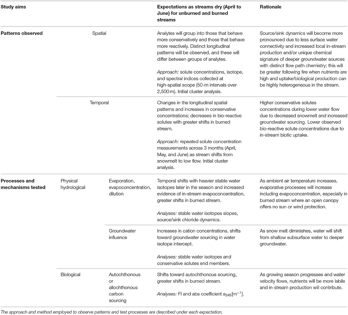
Table 1. Outlines the study framework and aims (left two columns under “Study aims” in bold outline), expectations, and rationale for stated expectations.

Methods

Experimental Design

Study Site

Our study took place at the Reynolds Creek Experimental Watershed (RCEW) and RC CZO, a 239 km² watershed located southwest of Boise, ID, USA. The USDA Agricultural Research Service (ARS) established RCEW in 1960 as an experimental watershed representative of the Intermountain West region in the United States (Marks et al., 2011), and the ARS has monitored long-term precipitation and stream discharge trends (Seyfried et al., 2000, 2018). The RCEW extends over a steep climatic gradient with mean annual precipitation varying from 250 to 1,100 mm/yr and mean annual temperatures from 5.5 to 11°C. This climatic variability is driven by the nearly 1,000 m elevation range. At lower elevations, rain is the dominant form of precipitation in the RCEW whereas snow is dominant at the highest elevations (Nayak et al., 2010; Kormos et al., 2014). Peak stream discharges across the watershed are driven by snowmelt patterns (Pierson et al., 2001). Vegetation includes Wyoming sagebrush steppe in the lower elevations, transitioning to mountain big sagebrush (Artemisia tridentata), antelope bitterbrush (Purshia tridentata), rabbitbrush (Chrysothamnus viscidiflorus), western juniper (Juniperus occidentalis), aspen (Populus tremulodes) and coniferous forest [mostly Douglas fir (Pseudotsuga menziesii)], at higher elevations (Seyfried et al., 2018). The site is underlain by Cretaceous granites and volcanic rocks such as the Miocene Salmon Creek Volcanics (McIntyre, 1972).

To evaluate spatial and temporal variation in stream chemistry, we studied two headwater streams within the RCEW known to be intermittent, Johnston Draw (basin area 1.83 km²) and Murphy Creek (basin area 1.32 km²; Seyfried et al., 2000; Pierson et al., 2001; Patton et al., 2018). Johnston Draw was ideal for this study owing to the availability of streamflow data measured at a dropbox v-notch 90° weir (Seyfried et al., 2000; Godsey et al., 2018). We opportunistically studied Murphy Creek to evaluate possible extremes in spatial and temporal variation in stream chemistry following wildfire. Specifically, the Soda Fire burned 68 km² of RCEW in August 2015, including Murphy Creek (Vega et al., 2020). Briefly, the fire was classified as moderate severity in the study area and consumed nearly all above-ground live vegetation resulting in more than 60% bare ground (bare soil, ash, and rock), with high sediment delivery to the stream (Vega et al., 2020). In October 2015, a dropbox v-notch 90° weir with pressure transducer for discharge measurements was re-activated in Murphy Creek. Hereafter we refer to Johnston Draw as “unburned JD” and Murphy Creek as “burned MC.”

Unburned JD and burned MC are comparable in basin area, discharge, elevation, mean annual precipitation (MAP), and aspect (Seyfried et al., 2000; Table 2). Annual water yields for 2016 were lower than the long-term average for both watersheds (Glossner, 2019). Though some studies find increased water yield after fire due to loss of vegetation (Atchley et al., 2018), in burned MC, the 2016 water year represented the third lowest streamflow year out of 12 years (1968–1977 and 2016–2017) of RC CZO data (Vega et al., 2020). The major differences between the two catchments are recent fire history and lithology (Table 2). The lithology of unburned JD is predominantly granodiorite with minor lithologic discontinuities including a combination of quartz latite and rhyolite flows underlying the high plateau at the top of the catchment, and a small olivine-rich basalt flow that extends into the outflow (McIntyre, 1972). Basalt and Salmon Creek Volcanics, underlies the burned MC. Unburned JD is described in more detail by Godsey et al. (2018) and Patton et al. (2018, 2019) and burned MC is described in more detail in Seyfried et al. (2000), Pierson et al. (2001), and Vega et al. (2020).

TABLE 2

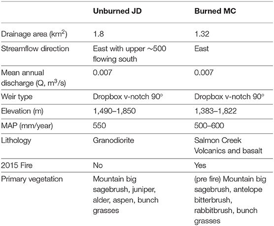
Table 2. Characteristics of the unburned JD and burned MC sub-catchments.

Sampling Design

To investigate spatiotemporal chemistry patterns in unburned JD and burned MC, we used a high-spatial scope approach: temporally repeated high-spatial density measurements at the km extent. In April, May, and June 2016, we sampled each stream at 50 m intervals (the grain of our study) over ~2,500 m distance (the extent of our study; Figure 1). Each 50 m site is referred to as a reach site (blue dots in Figure 1) and the reach sites span over ~2,500 m distance, the extent, which we refer to as the stream segment (Figure 1). In each stream segment, sampling started at the weir and continued to the uppermost observed surface flows (Figure 1) to include the entire sub-catchment. We refer to the suite of 50 m reach sites collectively as the stream longitudinal profile, and the spatial patterns identified using these sites as longitudinal patterns. Water samples were collected in pools at the stream thalweg following Dent and Grimm (1999).

FIGURE 1

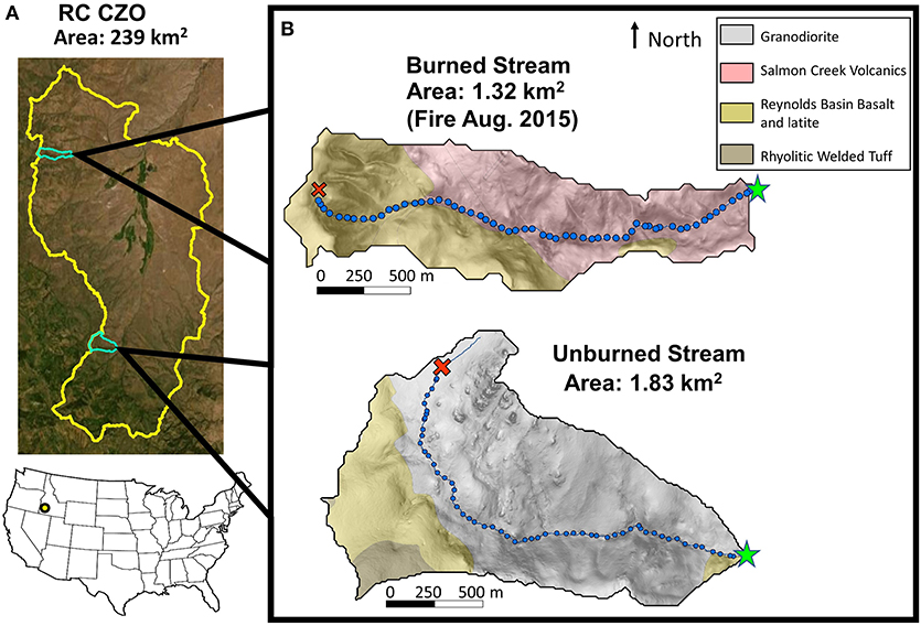
Figure 1. (A) Reynolds Creek Critical Zone Observatory (RC CZO) in southwestern, Idaho, USA (yellow dot). Outlined in turquoise are two headwater sub-catchments, unburned JD and burned MC, which are nested within the RC CZO, the perimeter of which is outlined in yellow. (B) Shows the study scope with the unburned JD (lower) and burned MC (upper) longitudinal sampling grain of 50 m interval, or stream reach sites (blue circles), spanning ~2,500 m extent. Longitudinal sampling sites start at a weir (green star) and extend to the uppermost reach with observed surface flow in each stream (red “x”), as identified in the field in April 2016. Colors indicate lithology based on McIntyre (1972).

Biogeochemical Characterization of Intermittent Streams

Physical and Chemical Field Properties

We characterized each stream reach site by measuring a suite of in situ properties including temperature (°C), pH, dissolved oxygen (DO mg/L), and estimated canopy cover. Water temperature (°C) and pH were measured at each stream reach site using an Oakton pH 110 Series probe (Vernon Hills, IL) calibrated with 4, 7, and 10 pH standard solutions; DO was similarly measured at each reach site with a YSI dissolved oxygen probe (Burlington, VT). Canopy cover was visually estimated in July at half of the stream sites using upward-oriented fisheye lens photos at pool height. Maximum canopy coverage was estimated at alternating sites from photos taken during full leaf-out. Canopy coverage was categorized based on the proportion of the photo covered by foliage (0–25, 25–50, 50–75, and 75–100%). Discharge (m³/s) was calculated from continuous stage measurements using a stage-discharge rating curve only at the outlet weir of each stream segment (Figure 1B). We acknowledge that direct measures of discharge and associated water balance at stream reach site would have augmented our understanding of stream dynamics and local water balance, but this was beyond this study. Accurately measuring discharge throughout a stream network at low flows is methodologically challenging and time-consuming. Instead, we focus here on concentration patterns and use indirect and environmental tracer approaches described below to understand inputs to and outputs from each reach site.

Surface Water Collection

To establish biogeochemical patterns in each stream, we collected surface water samples in the field and then filtered and analyzed them in the lab for the concentrations of a suite of chemical constituents. In the field, samples were collected in 250 mL amber high-density polyethylene bottles (HDPE) bottles, which had been rinsed three times and pre-leached in 18.2 MOhm distilled (DI) water. Bottles were then rinsed three times in the field with the stream sample and then filled to eliminate headspace. Samples were transported by backpack out of the steep terrain (~35–60 total per stream per sample period), and the water samples were kept refrigerated (4°C) until filtered and analyzed. For carbon and total nitrogen (TN) analysis, water samples were filtered within 72 h (typically within 24 h) in the lab using vacuum filtration through pre-combusted 0.7 μm Whatman glass fiber filters (GFF) into DI- and sample-rinsed 60 ml amber HDPE bottles. Amber HDPE bottles were used instead of glass owing to transport hazards (Sanderman et al., 2009). The remaining sample was syringe-filtered through a 0.45 μm Puradisc nylon filter into four 60 ml clear HDPE bottles for analysis of nutrients, anions, cations, isotopes, and fluorescence index. Samples were collected moving from downstream to upstream to minimize disturbance.

Laboratory Analysis

Stream chemistry was analyzed for a suite of chemical constituents, including dissolved inorganic carbon (DIC), DOC, TN, nutrients including ammonium-N, nitrate (${\text{NO}}_3^{-}$-N), orthophosphate (${\text{PO}}_4^{3-}$-P), anions including chloride (Cl⁻) and sulfate (${\text{SO}}_4^{2-}$), and cation concentrations including base cations and rare earth elements such as strontium (Sr). In addition, we analyzed stream water for stable water isotopes (δ¹⁸O and δ²H), fluorescence index (FI), and absorbance coefficient (a₂₅₄ [m⁻¹]. FI and a₂₅₄ methods are discussed in the DOC sourcing section. DIC, DOC and TN concentrations were measured on a Shimadzu TOC-V CSH (Columbia, MA, USA) equipped with an ASI-V autosampler and TNM-1 chemiluminescence detector for TN. Errors <2–3% were accepted for concentrations >1 mg C/L. High DIC concentrations (~10–30 mg DIC/L as C) resulted in difficulty using the non-purgeable organic carbon method (NPOC). Thus, we calculated DOC as the difference between TC and DIC and propagated the errors associated with this calculation (~0.3–0.9 mg/L). Cross validation of our DOC values with the Perdrial Environmental Biogeochemistry Lab at the University of Vermont (Burlington, VT) showed reasonable agreement (n = 140, r = 0.65). Owing to the higher error associated with DOC by difference, we approached DOC concentrations with some caution but retained them because DOC and spectral characteristics showed similarly variable patterns, and DOC provided an interesting contrast to other nutrients and DIC. Nutrients were measured on a Westco Discrete Analyzer (Unity Scientific, Brookfield, CT, USA), an automated chemical spectrophotometer. We accepted a <10% error for ${\text{NO}}_3^{-}$ -N and ${\text{PO}}_4^{3-}$ -P concentrations <1 mg/L and a 20% error for ${\text{NH}}_4^{+}$ -N <0.10 mg/L. For most of the analyses, we utilize TN because both ${\text{NO}}_3^{-}$ and ${\text{NH}}_4^{+}$ were below detection limit, with the exception of early season samples and those from burned MC. Anions Cl⁻ and ${\text{SO}}_4^{2-}$ were analyzed on a Dionex ion chromatograph (ICS-5000, Sunnyvale, CA, USA) with AS18 column 4 X 250 mm, and we accepted <10% error for sample <1 mg/L and 2–3% for samples > 1 mg/L. Cations were measured by the Center for Archaeology, Materials and Applied Spectroscopy (CAMAS) lab (Idaho State University, Pocatello, ID) on a Thermo X-II 283 series Inductively Coupled Plasma Mass Spectrometer (ICP-MS) equipped with a Cetac 240-position 284 liquid autosampler (ThermoFisher Scientific). Dilutions were 1:10 sample to de-ionized water. Some cations were below the detection limit of 10 ppb. We reliably measured Sr, Ba, Na, Mg, Al, Si, K, Ca, Sc, Ti, Fe, and Zn for all 3 months. Lastly, stable water isotope samples were analyzed at ISU/CAMAS Stable Isotope Laboratory on a Thermo Scientific, High Temperature Conversion Elemental Analyzer (TC-EA) interfaced to a Delta V Advantage mass spectrometer. Precision for both δ¹⁸O and δ²H was better than ± 0.2%0 and ± 2.00%0 respectively.

Lastly, autochthonous and allochthonous DOC sourcing was investigated by analyzing the spectral characteristics of DOM in the lab, specifically Fluorescence Index (FI) and absorbance. Completed by the Perdrial Environmental Biogeochemistry Lab at the University of Vermont (Burlington, VT), these characteristics were measured using the Aqualog Fluorescence and Absorbance Spectrometer (Horiba, Irvine, CA, USA). The excitation (EX) wavelength range spanned from 250 to 600 nm (increment 3 nm) and emission (EM) ranged from 212 to 619 nm (increment 3.34 nm). All excitation emission matrices (EEMs) were blank-subtracted (nanopure water, resistivity 18 MΩ cm⁻¹), corrected for inner filter effects, and Raman-normalized (Ohno, 2002; Miller et al., 2010). All samples were diluted to absorbance values below 0.3 and we computed relevant indices, including the FI (calculated as the intensity at Emission 470 nm divided by the intensity at Emission 520 nm for Excitation at 370 nm (Cory and McKnight, 2005). Absorbance (a) at 254 nm can also be used as a direct measure of aromaticity of DOM. We report the absorption coefficient (a₂₅₄ [m⁻¹]) which is calculated independently of DOC concentrations and using Equation 1 (Green and Blough, 1994; Inamdar et al., 2012) below:

$\begin{array}{ll}{a}_{254}[{\text{m}}^{-1}]=(\text{UV absorbance at }254\text{nm})\times 2.303\times 100.& (1)\end{array}$

Even though specific UV absorbance (SUVA₂₅₄) is the most commonly used indicator for DOM aromaticity (Weishaar et al., 2003), we refrained from its use due to the high error in DOC measurements and report a₂₅₄ [m⁻¹] instead.

Spatiotemporal Pattern Analyses

Initial Clustering of Water Properties and Biogeochemistry

To assess possible common synchronous or asynchronous drivers of biogeochemistry, we initially identified chemical variables within each stream that were strongly and weakly related over time using cluster analysis. We explored highly correlated groupings among chemical variables described above using cluster variable analysis for each month in order to understand a given variable's relationship with other variables over time. The loaded variables were the chemical properties and analyte concentrations measured in the field and lab including temperature, pH, DO, carbon (DIC and DOC), anions (Cl⁻), nutrients (TN and ${\text{PO}}_4^{3-}$), all cations measurable across the 3 months (Sr, Ba, Na, Mg, Al, Si, K, Ca, Sc, Ti, Fe, and Zn), and stable water isotopes (δ¹⁸O and δ²H). The cluster variable analyses were conducted in JMP (version 14.2) which first grouped variables into cluster components determined by first and second principal components and then ranked variables within cluster components based on the strength determined by a cluster algorithm (SAS Institute Inc., 2017). This algorithm iteratively clusters variables based on a combination of strength of the principal component and relative eigenvalue strength. The order in which the analytes and chemical properties are reported within each cluster is based on the highest Pearson correlation coefficient (r) within the cluster. The results of these analyses informed our choice of analytes used for longitudinal pattern reporting and testing our specific process hypotheses. We chose analytes that juxtapose each other by selecting both highly ranked variables within clusters of strongly temporally correlated variables as well as analytes that were not strongly clustered. We did this in order to represent a spectrum of more conservative solutes such as Cl⁻ to more biological reactive ones such as TN in each stream. The above criteria supported reporting longitudinal patterns for DIC, Cl⁻, Sr, DOC, TN, and ${\text{PO}}_4^{3-}$. However, we assessed temporal patterns from April to June in all chemical properties and solutes as well.

Longitudinal Spatial Patterns and Temporal Tendencies

To explore the biogeochemical patterns both along the length of the stream and monthly changes as the stream dried, we plotted the longitudinal patterns of all solutes for each month, but focused on those identified above in the cluster analysis: DIC, Cl⁻, Sr, DOC, TN, and ${\text{PO}}_4^{3-}$. These analytes also represent more conservative analytes and more reactive analytes as defined by Baker and Webster (2017). Stream data collected longitudinally from non-perennial streams presented challenges. First, samples collected 50 m apart in a stream are not statistically independent, second as streams dried April to June, it was impossible to sample in some locations and stream sample sizes changed, and third underlying longitudinal patterns complicated typical methods of quantifying spatial heterogeneity (details in statistical challenges of stream drying discussion section). Overall temporal comparisons of chemical properties, solutes, and cations from high to low flow were analyzed using mean differences and propagated errors from April to June within each stream. We determined differences to be substantial when they were larger than errors. As detailed above (Table 1), we expected to observe longitudinal and temporal similarities in both streams from April to June and predicted higher concentrations of carbon with evapoconcentration, lower concentrations of nutrients as in-stream primary production seasonally increased, and increasing cation concentrations as both streams became increasingly groundwater-dominated. However, we expected differences between the two streams like higher TN due to fire and higher cation loss due to volcanic lithology in burned MC.

Explaining Patterns: Testing Hypothesized Processes

Evaporative Processes

The potential evaporative signature of stream water was assessed by plotting stable water isotopes δ¹⁸O and δ²H against the Global Meteoric Water Line (GMWL) as well as the Local Meteoric Water Line (LWML; δ²H = 7.1(δ¹⁸O)-6.3), with data derived by Tappa et al. (2016). We compared monthly δ¹⁸O and δ²H data within each stream to the LMWL and calculated the monthly best-fit slopes based on simple linear regression and the LMWL-intercepts. To test for statistical differences between months and streams, we ran t-tests on the slopes of the regressed isotopic relationships. We hypothesized that the streams would undergo evaporation with drying in this semi-arid system (Fritz and Clark, 1997), and thus, that streams' isotopic data would fall below the LMWL (Gat, 1996). In addition, we predicted both streams would exhibit an increasingly evaporative signature as the streams dried, with a stronger shift in burned MC.

We evaluated the role of in-stream evapoconcentration in explaining chemistry patterns associated with stream drying by comparing the behavior of δ¹⁸O to Cl⁻ between upstream and downstream sites. We calculated predicted downstream values of Cl⁻ concentration ([$C{l}_D^{-}$]) based on ratios of δ¹⁸O from upstream (subscript “U” in Equation 2) and downstream (subscript “D”) samples and the observed upstream Cl⁻ ([$C{l}_U^{-}$]) values (Mulholland and Hill, 1997; Gallo et al., 2012):

$\begin{array}{ll}\left[C{l}_D^{-}\right]=\frac{\left[C{l}_U^{-}\right]\left[\delta 18O_D\right]}{\left[\delta 18O_U\right]}& (2)\end{array}$

Because both δ¹⁸O and Cl⁻ are expected to be conservative tracers (Baker and Webster, 2017), Equation 2 should lead to accurate predictions of Cl⁻ and each downstream site unless evapoconcentration or flushing were dominant processes. Therefore, we compared the predicted [$C{l}_D^{-}$] and observed Cl⁻ concentrations for each downstream site. If evapoconcentration were driving patterns in the water samples, we would expect to observe differences in the predicted vs. observed Cl⁻ concentrations. To explain any differences, we would need to parse out the role of flushing vs. evapoconcentration (Gallo et al., 2012).

Groundwater Influence

We used water isotopes and the Sr/DIC ratio to evaluate the potential influence of groundwater as streams dried. First, we calculated unburned JD's and burned MC's isotopic intercepts with the LMWL (Tappa et al., 2016) using each monthly regression (Fritz and Clark, 1997) and evaluated temporal shifts. We then compared the stream's LMWL-intercepts to the mean rain, snow, and groundwater samples collected by Radke et al. (2019) in a nearby but higher elevation watershed within RC CZO (Reynolds Mountain East ~2,100 m elevation). In this way, isotopic means of rain (δ²H −66.5 ± 12.7 and δ¹⁸O −8.4 ± 2.4, mean ± SE), snow (δ²H −129 ± 10.2 and δ¹⁸O −16.8 ± 1.3, mean ± SE) and groundwater samples (δ²H −121 ± 1.04 and δ¹⁸O −16.4 ± 0.18, mean ± SE) were assumed to be reasonable endmembers for our sites as well. As the streams dried, we expected the stream-LMWL intercepts to shift toward the groundwater signature later in the season if groundwater made up a larger component of the streams' surface water.

We also plotted Sr against DIC for each month because a previous study showed Sr to be a good indicator of groundwater at the RC CZO (Radke et al., 2019). We calculated RC CZO groundwater and precipitation (rain and snow) averages from samples collected by Radke et al. (2019) in late summer (August 2017), and used these values as endmembers in our analysis. Sr averaged 142.74 ± 8.77 ppb (mean ± SE) and DIC averaged 21.20 ± 0.55 mg C/L (mean ± SE). Rain and snow water samples had average values of 1.37 ± 1.63 ppb (mean ± SE) and 1.54 ± 1.80 mg C/L (mean ± SE) for Sr and DIC, respectively (Radke et al., 2019). We compared the upstream/downstream Sr-DIC relationship by comparing the uppermost 1,000 m sites with those in the lowest 1,000 m. We expected to observe a shift toward the groundwater ratio reflected in the late summer Sr/DIC ratios in unburned JD and burned MC that would be consistent with the shift in isotopic signatures.

Autochthonous or Allochthonous DOC Sourcing

Allochthonous carbon can be spectrally distinguished from autochthonous due to the structural carbon components in terrestrial vegetation, like lignin, which are also more aromatic. FI and a₂₅₄ [m⁻¹] measure these spectral components and help classify carbon sources as allochthonous or autochthonous (McKnight et al., 2001; Inamdar et al., 2012). We compared FI to published ranges of these values associated with more autochthonous or allochthonous sources (Inamdar et al., 2012). Based on these values, we interpreted FI values between 1.2 and 1.5 as reflecting an allochthonous signature whereas FI above 1.7 reflects an autochthonous/microbial signature (McKnight et al., 2001). Furthermore, we report the variability using coefficient of variation (CV) because FI had no underlying longitudinal patterns in either stream (see discussion section, “Statistical Challenges of Stream Drying Data”). However, in our calculations, we controlled for sample size in each stream by including only those sites that had water flowing all 3 months so as not to bias any one month.

Aromatic and humic DOM is a product of terrestrial vegetation so that a higher aromatic a₂₅₄ signature reflects a more allochthonous DOM with structural carbon. Thus, the relationship between FI and a₂₅₄ is inverted, such that lower a₂₅₄ result from less aromatic DOM, more autochthonous/microbial derived carbon and higher a₂₅₄ result from more aromatic, more allochthonous derived carbon (Inamdar et al., 2012). Due to increased in-stream primary production as both streams dried, we expected to observe FI to increase reflecting shifts from more allochthonous to autochthonous carbon, and a₂₅₄ to decrease reflecting diminished aromatic properties with a more pronounced shift in burned MC.

Results

Biogeochemical Characterization of Intermittent Streams

Stream Hydrologic Conditions

Seasonal drying in both intermittent headwater streams was similar, with weir discharges (Q) decreasing in April, May, and June 2016 (Figure 2A). Drying occurred in both streams between April and June. For unburned JD, all of the April sampling sites (n = 57) had surface flow, 89% persisted in May (n = 51), and only 65% sustained surface flows in June (n = 37). Drying occurred in reaches interspersed throughout the unburned JD stream. Similarly, all of the reach sites in burned MC were flowing in April (n = 59), but only 73% in May (n = 43), and 64% sustained flow in June (n = 38). Unlike in unburned JD, drying in burned MC occurred from the top of the stream to the bottom as though the entire stream contracted longitudinally (though subsequent work showed this pattern did not persist later in the summer; Warix, 2020). Thus, by June, 35% of unburned JD's and 36% of burned MC's reach sites had dried, with the highest proportion of sites drying from May to June in unburned JD stream and from April to May in burned MC stream. Over the sample period, unburned JD stream discharge exhibited a slightly greater relative change (April Q ~ 0.022 m³/s to June Q < 0.005 m³/s) than burned MC (April Q ~0.017 m³/s to June Q ~0.005 m³/s; Figure 2A). Burned MC also exhibited flashier stream flow as spikes in discharge, presumably responding to event-based precipitation or snowmelt inputs (Figure 2A) that did not occur as strongly in unburned JD.

FIGURE 2

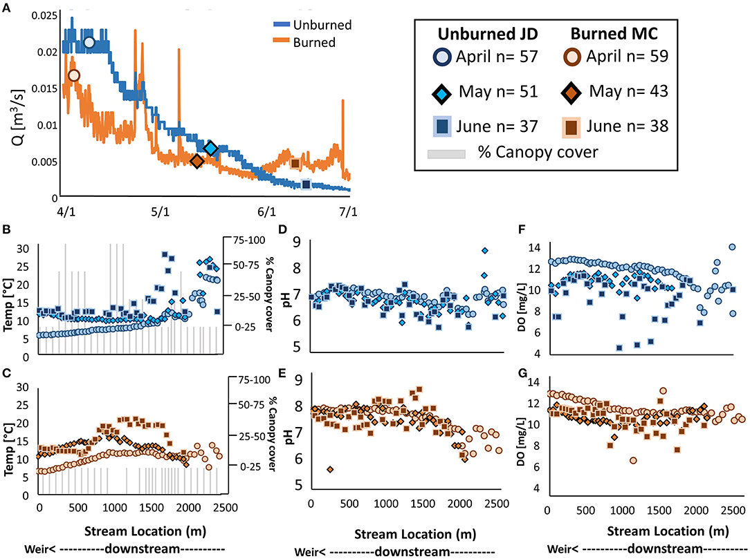
Figure 2. 2016 discharge (A) of the unburned JD (blue) and burned MC (orange) measured at the weir (most downstream sample point); symbols reflect the discharge on the sample dates. Longitudinal patterns of (B,C) temperature (°C) and estimated canopy cover (% cover in gray bars) (D,E), pH (-log [H+]), and (F,G) dissolved oxygen (DO mg/L).

Physical and Chemical Field Properties

The streams were similar in physical and chemical properties measured in the field but as expected, canopy cover differed between the unburned stream and burned stream. Stream temperature showed strong longitudinal and increasing temporal shifts in both streams, whereas pH and DO were more variable longitudinally and temporally (Figures 2B–G and Supplementary Table 1). The two streams differed in canopy cover in that 44% of unburned JD had >25% canopy cover during full leaf-out whereas 100% of sites sampled in burned MC had <25% canopy cover, and most sites fell very close to 0% canopy cover even in July 2016 (Figures 2B,C). Although some burned MC sites had >0% canopy cover in July, the post-fire vegetation differed from the vegetation in the unburned JD. The riparian vegetation of burned MC in July was dominated by fast-growing, non-woody shrubs and small, young willows because all vegetation, namely sagebrush and bunch grasses were charred to the ground (Vega et al., 2020). This contrasted with the overhanging riparian alder, willow, and juniper in unburned JD.

Biogeochemical Pattern Analysis

Initial Clustering of Water Properties and Biogeochemistry

Correlations between stream analytes varied between streams and these relationships changed as each stream dried. We identified groups of solutes that behaved similarly or dissimilarly for each stream at different moments in the season. For example, in unburned JD, we observed positive correlations between Sr, Mg, Ca, K, Na, Ba, Fe, DOC, temperature (Temp), DIC, δ¹⁸O, TN, Cl⁻, Sc, and Si in April. Ti, Al, DO, pH, ${\text{PO}}_4^{3-}$, and Zn were negatively correlated with these analytes and chemical properties, but positively correlated with each other (Figure 3A). By June, Mg, Fe, Cl⁻, K, Temp, TN, δ¹⁸O, Sc, and Si were positively correlated with each other, but shifted to being negatively correlated with other analytes or chemical properties. From April to June, shifts from negatively to positively correlated analytes were observed between Ti, DO, pH, and ${\text{PO}}_4^{3-}$ and other analytes or properties in unburned JD (Figure 3E). We observed similar (though not identical) patterns within burned MC (Figures 3B,D,F). Strongly correlated (either positively or negatively) analytes were placed into clusters for each month and stream (Supplementary Table 2). Based on these results, we selected representative analytes to illustrate different clusters and behaviors for the longitudinal analysis, including DIC, DOC, TN, ${\text{PO}}_4^{3-}$, Sr and Cl⁻.

FIGURE 3

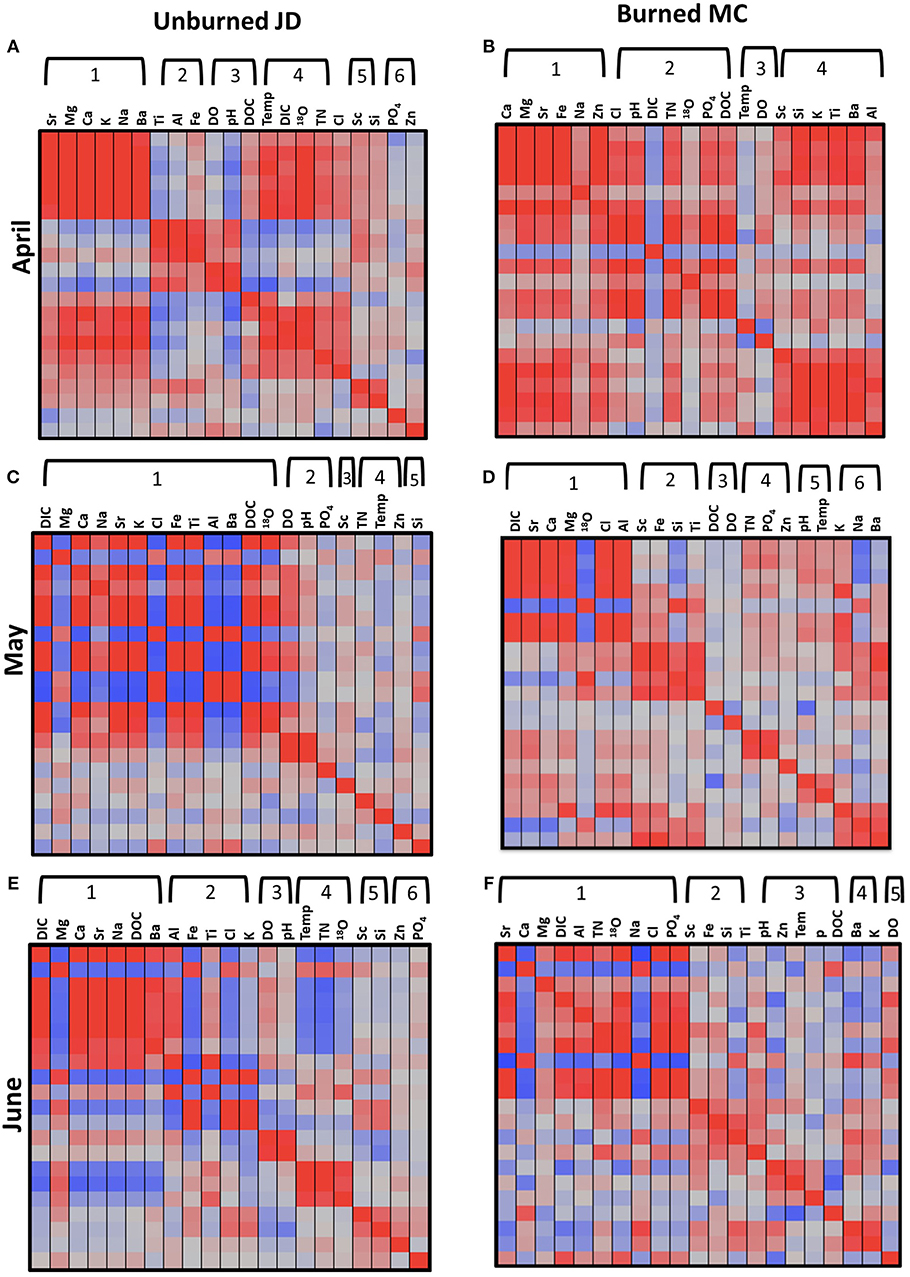
Figure 3. Cluster analysis shows correlations between analytes by rows for April (A,B), May (C,D), and June (E,F) for unburned JD (left column) and burned MC (right column). Analytes include: temperature, or Temp (°C), DO (mg/L), pH, DIC (mg C/L), Cl⁻ (mg Cl/L), DOC (mg C/L), TN (mg N/L), ${\text{PO}}_4^{3-}$ (mg P/L), δ¹⁸O, and cations (ppb): Sr, Ba, Na, Mg, Al, Si, K, Ca, Sc, Ti, Fe, and Zn. Analytes are labeled across the top of each x-axis and are listed in the same order along the y-axis in each panel. Analyte order is based on cluster analysis groupings where analytes within each cluster are more strongly correlated (higher Pearson correlation coefficient or r-value) to each other than to other groups of analytes. The r-values are colored by saturation where the higher the r-value, the more saturated the color, and gray represents a low r-value and low correlation. Red indicates positive correlations and blue negative correlations.

Longitudinal Spatial Patterns

Common longitudinal patterns were evident in both unburned JD and burned MC streams (Figure 4) for many of the more conservative analytes (e.g., DIC, Sr, and Cl⁻) than the biologically reactive ones (e.g., DOC, TN, and ${\text{PO}}_4^{3-}$). As expected, mean concentrations generally increased for DIC, Sr, and Cl⁻ downstream (Figures 4A–F). The exception to this pattern were consistently high concentrations at the top of unburned JD (relative to downstream concentrations) at reach sites that were south-facing and meadow-like. Concentrations of more reactive analytes, DOC, TN, and ${\text{PO}}_4^{3-}$, tended to decrease downstream in unburned JD whereas DOC and ${\text{PO}}_4^{3-}$ were relatively invariant longitudinally in the burned MC stream. TN was exceptional in that it varied in the uppermost portions of both streams with patterns that changed each month of the sampling campaign.

FIGURE 4

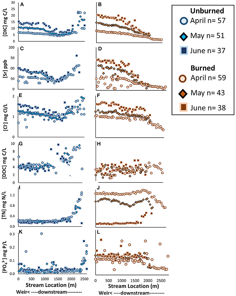
Figure 4. Longitudinal patterns of (A,B) dissolved inorganic carbon (DIC mg C/L) (C,D), strontium (Sr ppb) (E,F), chloride (Cl⁻ mg Cl/L) (G,H), dissolved organic carbon (DOC mg C/L) (I,J), total nitrogen (TN mg N/L) (K,L), phosphate (${\text{PO}}_4^{3-}$ mg P/L) for unburned JD (blue, left column) and burned MC (orange, right column) streams. Values from April are represented by circles, May sites are diamonds, and June sites are squares along the length of the stream where 0 m is the weir and ~2,500 m is the upper stream reach.

Temporal Shifts

As expected, mean differences in concentrations between April and June showed that TN concentrations substantially decreased over the growing season in each stream, and by an order of magnitude in burned MC (Figure 5B). Mean TN concentration decreased by >80% from April to June (Figure 5B) in burned MC stream (1.14 ± 0.03 to 0.19 ± 0.02 mg N/L, mean ± SE); TN was composed mostly of ${\text{NO}}_3^{-}$; even in April, ${\text{NH}}_4^{+}$ was largely below our instrument detection limit. We observed a similar but less pronounced decrease in TN in unburned JD (Figure 5A), where a 39% decrease occurred over the same months (0.36 ± 0.04 to 0.22 ± 0.03 mg N/L, mean ± SE). Unlike TN, ${\text{PO}}_4^{3-}$ decreased only slightly in the burned MC stream over the growing season and did not exhibit a measurable change in unburned JD (Figures 5A,B and Supplementary Table 3). In contrast to our expectations, DOC exhibited no clear temporal shift from April to June in unburned JD and slightly decreased in burned MC (Figure 5).

FIGURE 5

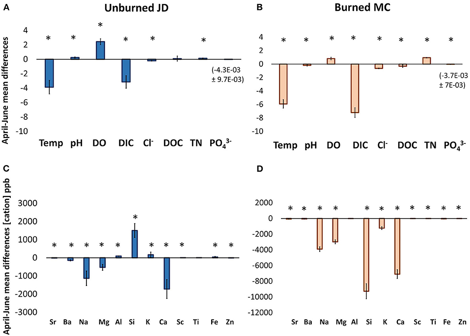
Figure 5. Mean solute differences from April to June are shown for (A) unburned JD and (B) burned MC for temperature, or Temp, (°C), pH (-log [H+]), DO (mg/L), DIC (mg C/L), DOC (mg C/L), TN (mg N/L), ${\text{PO}}_4^{3-}$(mg P/L), Cl⁻(mg Cl/L), DOC (mg C/L), TN (mg N/L), ${\text{PO}}_4^{3-}$(mg P/L). Mean cation differences (ppb) from April to June are shown for unburned JD (C) and burned MC (D). Error bars show propagated error and asterisks indicate where differences are greater than the propagated error. Positive differences indicate decreasing in concentration from April to June and negative differences indicate increasing concentration from April to June (arrows for reference). Note pH measures are representative of log scale, so small changes are not equivalent to raw concentrations of other solutes. Additionally, please note the difference in axes scales between panel (C,D).

In both streams, we observed similar temporal patterns in the average differences from April to June for base cations and other solutes (Figures 5C,D). Like DIC and Cl⁻, most cations increased from April to June in both streams as indicated by negative difference values between April and June mean concentrations (Figures 5C,D). However, in unburned JD, some cation concentrations decreased as indicated by positive difference values as was the case for Si, Fe, and Ba. As expected, burned MC exhibited three to ten times larger cation differences than unburned JD for several cations including Na, Mg, Si, K, and Ca (Figures 5C,D and Supplementary Table 4).

Explaining Patterns: Testing Hypothesized Processes

Evaporative Processes

Isotopic signatures for both streams showed that evaporation was occurring, which we expected. However, counter to our predictions, we did not find evidence of temporal shifts toward increasing evaporation with stream drying in either stream. The regression slopes of the δ¹⁸O-δ²H relationships for all months for both unburned JD and burned MC fell below the GMWL and LMWL (Tappa et al., 2016), indicating an evaporative signature in these two streams compared to local precipitation (Figures 6A,B). In the unburned JD, we observed a lower-sloped evaporative trend with drying as April's slope (± SE) was 2.7 ± 0.16, May's was 3.6 ± 0.27, and June's slope 4.7 ± 0.30 (Table 3). All months within unburned JD were statistically different so that April differed from May (t = −5.2, p = < 0.0001, df = 103), May differed from June (t = −4.4, p = 3.7E-05, df = 81), and April from June (t = −14.14, p = < 0.0001, df = 84). In the burned MC stream, April's slope (± SE) was 4.3 ± 0.30, May's was 3.0 ± 0.26, and June's was 4.5 ± 0.23 (Table 3). In contrast to unburned JD, burned MC slopes for April and June did not statistically differ from each other (t = −0.51, p = 0.61, df = 91), although both differed from May (t = −2.6, p = 0.01, df = 95 and t = −5.1, p = < 0.0001, df = 76, respectively), which had the most evaporative signature over the study period. Between the two streams, slopes were only significantly different from each other in April (t = −10.24, p = < 0.0001, df = 108) and not in May (t = 1.0, p = 0.32, df = 89) or June (t = 0.6, p = 0.56, df = 70). We generally did not observe longitudinal patterns of evaporation (Figures 6A,B), with the exception of the uppermost portion of unburned JD. There, the aspect and vegetative cover of the stream was distinct from downstream reaches: these south-facing meadow sites had a strong evaporative signature in April (Figure 6A) and had dried by May.

FIGURE 6

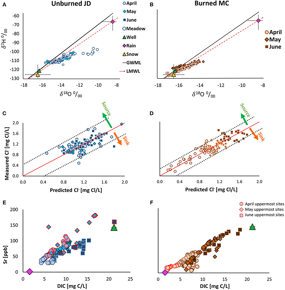
Figure 6. Stable water isotopes (δ¹⁸O and δ²H) for sites in both unburned JD (A) and burned MC (B) in April (light circles), May (mid-tone diamonds), and June (dark squares). The global meteoric water line (GMWL) is shown in solid black and the local meteoric water line (LMWL) is the dashed red line (δ²H = 7.1(δ¹⁸O)-6.3; Tappa et al., 2016). Mean rain (pink diamond), mean snow (yellow triangle), and mean well values (green triangle) samples were collected by Radke et al. (2019) at a higher elevation site in Reynolds Creek watershed. Measured vs. predicted Cl⁻ concentrations calculated using δ¹⁸O upstream and downstream site ratios for the unburned JD (C) and the burned MC (D). Red solid line represents identical measured and predicted concentrations and the dashed gray lines enclose the prediction interval. Cl⁻ values above the red line indicate Cl⁻ concentrations greater than expected (potential source) and Cl⁻ concentration below the red line indicate Cl⁻- values that are less than expected (potential sink). Sr and DIC relationships for the unburned JD (E) and the burned MC (F). Mean precipitation (both snow and rain) and mean groundwater endmembers from Radke et al. (2019) are represented by pink diamonds and green triangles, respectively. Gray bars on endmembers show the SE. Uppermost reach sites (>2,000 m) of each stream are outlined in red for each month water was present.

TABLE 3

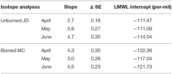
Table 3. The slope ± standard error and the LWML-intercept extracted from the data presented in Figures 6A,B.

In-stream Evapoconcetration or Dilution Influences on Solute Concentrations

To investigate potential effects of evaporation or dilution on the concentration of solutes as streams dried, we evaluated source-sink dynamics of chloride compared to δ¹⁸O. In both streams, most measured Cl⁻ fell within the error of the predicted Cl⁻ based on δ¹⁸O, indicating the two analytes behaved conservatively, with no major new gains or losses of water. Given this finding, we did not further investigate spatial or temporal deviations due to either evapoconcentration or dilution (Figures 6C,D). Although we hypothesized that in-stream evapoconcentration would be a driver of increased analyte concentrations, we found few sites in either stream that showed concentrations outside of the δ¹⁸O-based prediction intervals. Additionally, counter to our predictions, we observed no differences between streams despite their difference in canopy cover.

Groundwater Influence

The isotopic signature of both streams showed surface water sources to be mixed contributions of snowmelt and rain: each stream's isotope values fell between the snow and rain mean values reported by Radke et al. (2019; Figures 6A,B). Based on intercepts, water in both streams had dominant contributions from snow/groundwater; snow sources for unburned JD reflected a larger rain contribution as indicated by isotopic-intercepts with the LMWL (~−111 δ²H per mil) whereas the LMWL-intercept for burned MC stream (~−120 δ²H per mil) reflected a larger snow and/or groundwater contribution (Figures 6A,B). Because the groundwater and snow isotopic signatures were similar, we could not distinguish between the two sources with isotopic tracers. Counter to our expectations, no clear temporal shifts in water sources emerged in the isotope data in either stream (Table 3).

However, temporal shifts in groundwater-precipitation mixing were apparent by pairing the isotopic patterns with observed shifts in DIC and other analyte concentrations. For example, we observed that DIC and Sr were strongly correlated (Figure 3). When compared to the average precipitation (rain and snow) and late summer groundwater Sr/DIC endmembers, stream water was sourced from precipitation in April and shifted toward groundwater sourcing in June in each stream (Figures 6E,F). In contrast to isotopes of water, rain and snow precipitation had similar DIC and Sr signatures and these signatures were substantially different from groundwater DIC and Sr signatures (Radke et al., 2019). We likely did not capture an additional endmember in unburned JD in the upper portion of the catchment (Figure 6E) whereas most of the variation in the burned MC was captured by two endmembers, potentially with exception of a few downstream sites (Figure 6F). The uppermost reach sites (>2,000 m) of each stream (flowing in April and May) had different signatures; the signatures from the upstream reaches in unburned JD fell close to groundwater and burned MC upstream reach sites fell close to a precipitation signature (Figures 6E,F and Supplementary Figure 1).

Organic Carbon Sourcing: Autochthonous and Allochthonous Processes

DOM sources and spectral characteristics varied along the profile of each stream during each month; FI varied by similar amounts in both streams whereas a₂₅₄ [m⁻¹] varied more in unburned JD (Figure 7). Many FI values fell between the 1.5 allochthonous derived threshold and the 1.7 autochthonous/microbially derived threshold (Figures 7A,B), indicating mixed carbon sources in both streams. Unburned JD had a slight but surprising longitudinal FI pattern in April (mean 1.59 ± 0.01 SE) when we observed a more autochthonous/microbial FI signature downstream, while the upper reach of the stream had a more allochthonous signature (Figure 7A, circles). May generally had an allochthonous signature (mean 1.49 ± 0.003 SE) as did June (mean 1.50 ± 0.007 SE), and this similarity between seasons was counter to our predictions. Interestingly, while May and June mean FI values were similar, June exhibited greater variation (CV 2.8) than May (CV 1.2), with points spanning the thresholds between autochthonous and allochthonous sources in both months (Supplementary Table 5).

FIGURE 7

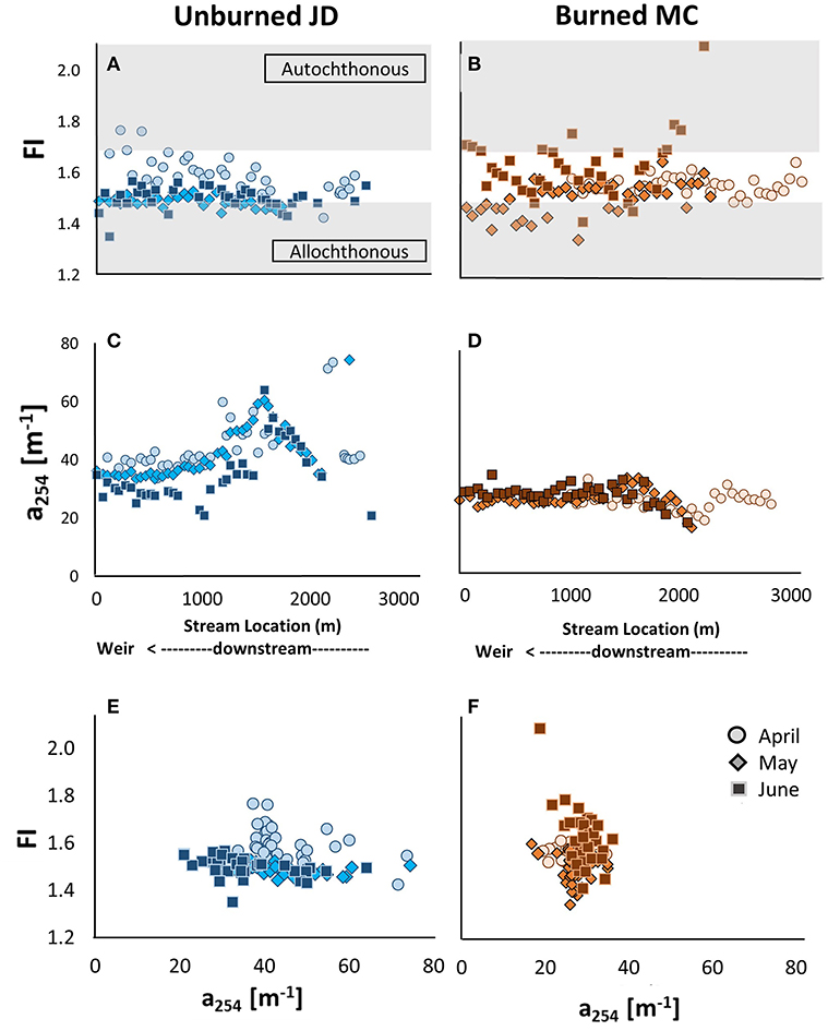
Figure 7. (A,B) Fluorescence index (FI) (C,D), absorbance coefficient (a₂₅₄ [m⁻¹]), and (E,F) the relationship of FI to a₂₅₄ for stream profile of unburned JD (blue, left) and burned MC (orange, right); shape, shade, and color of months are described in Figure 2. Gray shaded boxes (A,B) indicate the 1.5-1.2 allochthonous-derived threshold and the 1.7–2.0 autochthonous/microbial-derived threshold.

In burned MC (Figure 7B), we observed a mixed autochthonous and allochthonous FI signature in April (mean 1.55 ± 0.005 SE), and a similar but more varied FI signature in May (mean 1.50 ± 0.009 SE). June's FI varied along the stream profile with an overall downstream increase toward autochthonous/microbial signature (mean 1.62 ± 0.02 SE). This tendency matched our expectations of increasing in-stream productivity, which we expected would be more pronounced in the burned stream. In addition, burned MC's higher mid-summer FI variation was reflected in the relatively high June FI CV (7.5) compared to that of April (1.0) and May (3.5; Supplementary Table 5). Despite the overall autochthonous tendency in June, there were also sites for which the FI value fell below or close to the allochthonous threshold (1.5, Figure 7B, squares). We did not expect to observe this high variation.

We expected that as streams dried, DOC aromaticity (high in terrestrially derived carbon) would be decreasing due to increased in-stream productivity, especially in burned MC, and thus, we expected decreases in a₂₅₄ values. Overall, unburned JD had higher a₂₅₄ values that were more longitudinally and seasonally variable than burned MC (Figures 7C,D and Supplementary Table 5). We expected higher overall aromaticity in unburned JD. Though we expected to see higher FI values coupled with low a₂₅₄ values, we did not observe these relationships consistently. In April, unburned JD had higher a₂₅₄ values (mean 44.5 ± 1.4 SE) coupled with higher FI values (Figure 7E). The unburned JD maintained higher a₂₅₄ values in May (mean 48.1 ± 3.0 SE) and dropped in June (mean 38.5 ± 2.9 SE); this decrease in aromaticity suggests less terrestrial carbon and followed our expectations. Compared to unburned JD, burned MC a₂₅₄ values shifted less from April (mean 26.2 ± 0.48 SE) to May (mean 27.2 ± 0.54 SE) and June (mean 29.1 ± 0.53 SE, Figure 7D). The differences in a₂₅₄ temporal patterns between the streams were illustrated by the relationship of FI and a₂₅₄ (Figures 7E,F) where the spread of FI values was greater in the burned MC, but the spread of a₂₅₄ was greater in the unburned JD. We hypothesized that increased in-stream productivity would result in shifts of increased FI and decreased a₂₅₄ values. However, the spatial patterns we observed in both streams were more longitudinally varied and had less clear seasonal shifts than expected.

Discussion

Stream intermittency and fire regimes are changing in the Intermountain West and cold montane shrubland ecosystems that characterize the northern Rocky Mountains and Great Basin are especially vulnerable to these changes. We hypothesized stream chemistry patterns would change seasonally and longitudinally in response to both drying and fire, and that process shifts would explain these biogeochemical patterns. Specifically, we hypothesized that with drying, in-stream evaporative processes, increased groundwater influence, and shifts in DOC sourcing from allochthonous to autochthonous would contribute to differences in these longitudinal stream chemistry patterns. In a recently burned watershed, we expected the impacts of these processes would be amplified.

Stream Drying: Non-linear Spatiotemporal Biogeochemical Patterns

Both streams exhibited non-linear longitudinal patterns in chemistry that changed with stream drying. Spatially variable and distinct patterns among analytes were revealed by this study's high-scope sampling approach and breadth of measured chemical constituents. For instance, we identified potential springs/deeper groundwater inputs where temperature or solute concentrations remained stable despite seasonal shifts at other locations longitudinally along the streams (e.g., around ~1,500 m in unburned JD and ~ 2,000 m in burned MC). In contrast to our expectations, we found similar longitudinal patterns and processes driving these patterns in both streams. This provides some evidence for emerging regional behavior in the subsurface processes (i.e., groundwater contributions) driving stream chemistry. Our findings collectively point to the power of high-scope sampling to capture both the temporal and spatial variability in intermittent stream processes, and they contribute empirical data on how spatiotemporal patterns and processes may change with stream drying in headwater streams like these.

Streams Similarities: DIC Dominance With Drying

Given the differences in fire history and lithology, the similarity of chemistry patterns and shifting processes between these two streams was surprising. In both unburned JD and burned MC, DIC and many cations exhibited clear longitudinal patterns that increased in mean concentration with stream drying. Though we did not directly analyze concentration-discharge relationships longitudinally at each 50 m reach site, chloride source/sink dynamics did not suggest strong spatial inputs or outputs in any month. Monthly increases in DIC and other conservative solute concentrations were consistent with dilution behavior of concentration-discharge observed over the water year at the weir of each stream (Glossner, 2019). While conservative solutes in larger streams often display chemostatic behavior (Godsey et al., 2009), our data is consistent with chemodynamic concentration-discharge relationships documented in smaller catchments (Hunsaker and Johnon, 2017) and intermittent streams (Bernal et al., 2019). Instead of evapoconcentration or dilution, our findings point to deeper groundwater sources driving increased concentrations as the streams dried. Our findings are consistent work by Wlostowski et al. (2020), whose findings describe loamy and sand-rich soils and relatively shallow bedrock in unburned JD resulting in more baseflow-dominated streamflow with less subsurface water storage compared to CZOs with clay-rich soils. Distinct from other baseflow dominated streams, groundwater contributed to low flow in our streams, not high flow as observed in the Jemez River Basin Critical Zone observatory in New Mexico (McIntosh et al., 2017). Our results build off of those reported by Radke et al. (2019) at a higher elevation RC CZO catchment during snowmelt, where deeper flow paths rather than shallow subsurface flow paths contributed to stream DOC as observed by Boyer et al. (1997). Deeper flow paths also contribute to increasing ion concentration patterns at low flow in Dry Creek Experimental Watershed near Boise, ID (McNamara et al., 2005). Our findings, along with these earlier works suggest a regional occurrence of limited near-surface storage capacity due to loamy soils and the importance of deeper groundwater for stream water.

In contrast to DIC, more biologically reactive solutes TN, DOC, and ${\text{PO}}_4^{3-}$ either decreased or were relatively invariant with stream drying. Mean TN concentrations decreased throughout the growing season, and DOC showed relatively high variability and no clear longitudinal pattern or large seasonal shift in either stream. With respect to TN, we expected temporal decreases because nitrogen is biologically reactive and often subject to uptake, especially during low flows and low concentrations (Moatar et al., 2017). On the other hand, many studies of stream carbon dynamics have found clear seasonal patterns in DOC (Hornberger et al., 1994; Boyer et al., 1997; Mulholland and Hill, 1997; McGuire et al., 2014; Hale and Godsey, 2019). However, we did not observe a strong DOC pattern with drying in either stream. Rather, we found strong temporal shifts in DIC, and DIC concentrations that were 2–3 fold higher than DOC in unburned JD and burned MC. Thus, DIC, rather than DOC, appeared to dominate stream carbon dynamics at our sites.

Non-linear spatial patterns in longitudinal stream chemistry spatial patterns have been observed in other studies that employed high spatial-scope measurements, but few have examined these longitudinal patterns in the context of stream drying or across such a broad suite of biologically reactive and conservative analytes. In one such example, within snowmelt-driven, deciduous forested streams at Hubbard Brook, NH, Likens and Buso (2006) sampled at 100 m intervals over a network and observed non-linear spatial patterns in a wide suite of constituents including DOC, DIC, K, Na, ${\text{SO}}_4^{2-}$, ${\text{NO}}_3^{-}$, Sc, dissolved Si, and Ca (also see McGuire et al., 2014; Zimmer and Lautz, 2014). Similarly, Dent and Grimm (1999) found that ${\text{NO}}_3^{-}$ -N and soluble reactive phosphorus (SRP or ${\text{PO}}_4^{3-}$) varied longitudinally in the hot desert at Sycamore Creek, AZ. Moreover, based on 25 m intervals over 10 km of stream, they observed that ${\text{NO}}_3^{-}$ -N decreased and SRP increased with succession following monsoonal flooding. These findings agree with our observations of decreasing TN concentrations and relatively invariant (unburned JD) or slightly decreasing ${\text{PO}}_4^{3-}$ (burned MC) with drying.

Stream Differences: Lithology and Fire Impacts

We found differences between the two streams we studied in cation concentrations, the proportion of open canopy, and magnitude of seasonal decrease in TN, organic carbon and water sourcing. Lithological differences likely account for higher cation concentrations in volcanic burned MC compared to granitic unburned JD stream (Meybeck, 1987; Ibarra et al., 2016). It is also likely that fire impacts increased cation concentrations through ash and sediment inputs and/or mineralization of these inputs, especially during snow melt. At the watershed scale, sediment losses were high during winter and snowmelt in the year following fire, a low flow year, and sustained in 2017 (>450 compared to 20 g m⁻² yr⁻¹ mean sediment yield in Johnston). Sediment losses were low during the drying summer months (<5% of annual sediment yield) indicating low contributions of particulates during this study period (Glossner, 2019); mineralization of these ash-derived products warrants further study.

Elevated nitrogen levels in April and May in burned MC decreased by >80% in June. These TN results supported our hypothesis that nitrogen levels would be elevated immediately following wildfire but that decreases in TN would be observed as burned MC dried due to potentially increased nutrient uptake. Other studies such as Murphy et al. (2006) and Rau et al. (2007) have documented that there is often a lag in nitrate uptake following fire due to the time required to re-establish uptake by denitrifying bacteria populations and vegetation. In some cases, high nitrogen levels have been documented in streams for years following fire (Hauer and Spencer, 1998; Mast et al., 2016), potentially related to low DOC from terrestrial carbon losses (Rodríguez-Cardona et al., 2020). However, TN levels in burned MC decreased relatively quickly to concentrations similar to those of unburned JD by June. Finally, DOM sourcing followed different temporal tendencies in the two streams: burned MC shifted as expected from more allochthonous to autochthonous whereas unburned JD showed more mixed contributions. These findings will be discussed further below in the “Statistical Challenges of Stream Drying Data”.

Fire can have a large effect on water budget and cause increases in stream flow as catchment ET diminishes following vegetation losses (Kinoshita and Hogue, 2015; Atchley et al., 2018), but we did not find strong evidence of this influencing stream chemistry drying patterns. This in part may be because burned MC experienced a relatively low water year in 2016 (Glossner, 2019; Vega et al., 2020) and rapid growth of grasses and herbaceous was observed. Rapid fire recovery (within a year) has been observed previously at RC CZO with regards to gross ecosystem production (Fellows et al., 2018) and ET (Flerchinger et al., 2016), with statistically marginal short-term increases to stream flow (Flerchinger et al., 2016). Moreover, ET rates have been shown to be relatively low in sagebrush in RC CZO (Sharma et al., 2020). Isotopic LMWL-intercepts indicated differing water sources between the streams and suggested unburned JD was more rainfed than burned MC, which was fed more by groundwater/snow. Given the vegetation differences, it is possible unburned JD had more shallow subsurface storage of rainwater than burned MC. However, as vegetation regrew in burned MC, there was no clear LMWL-intercept shift from April to June suggesting changes in soil water storage capacity. Alternatively, water source differences may have reflected pre-fire differences and further study would be required to parse this out. As mentioned, we observed stream chemistry responses to fire in some instances like elevated TN, but we did not detect increased stream flow. These observations are consistent with the weak evidence of monthly changes in evapoconcentration or dilution processes and burned MC's lack of shifts in water isotopic water sources or evaporative slopes. In addition to the similarity of stream patterns indicating the importance of deeper subsurface processes on stream chemistry, the similarity may indicate muted effects of fire on stream chemistry in the burned watershed.

Processes Explaining Spatiotemporal Patterns

Our findings highlight the utility of stream chemistry to elucidate both hydrological processes (evaopconcentration or dilution and water sourcing) and the in-stream biological processes (potential autochthonous carbon-sourcing) that contribute to spatiotemporal patterns as streams dry seasonally and following wildfire. A strength of our data was that we were able to evaluate surface-groundwater interactions, which has been identified as a key research priority to understanding intermittent stream controls (Costigan et al., 2016). Our inferences are only made possible by the high spatial scope sampling approach we employed.

Evaluating Hydrological Processes: Shift Toward Groundwater With Drying

By quantifying evaporation and groundwater influence, we could distinguish between chemistry drying patterns driven by surface processes and chemistry drying patterns driven by subsurface hydrologic processes in these streams. Isotopic slopes showed both streams were evaporative; however, we observed no temporal shifts toward increased in-stream evaporation with drying. Contrary to our expectations and despite differences in canopy cover, both streams showed similar evaporative trends in water isotopes with no statistical difference in slope between the two streams in May or June. Furthermore, we found only weak evidence of in-stream evapoconcentration or dilution on the spatial stream chemistry patterns in either stream during any month. In contrast, Sr-DIC ratios provided strong evidence that stream surface water shifted toward a deeper groundwater signature with drying. These low-flow groundwater contributions differ from the lateral input dominance of snowmelt described by Boyer et al. (1997). The Sr-DIC relationships varied longitudinally and were better captured by precipitation and groundwater endmembers in burned MC than unburned JD. In April, the Sr-DIC signature of the uppermost portion of unburned JD led us to reason that either that these sites are spring-fed or that our sampling missed the shift from precipitation to groundwater sourcing. In general, increased contact time between water and soil/bedrock may explain elevated cation and DIC concentrations in groundwater (Fritz and Clark, 1997; Richter and Billings, 2015; Olshansky et al., 2019), each of which increased with drying in both streams. Although isotope intercepts did not show strong shifts in water sourcing between months as Sr-DIC ratios did, the isotopic signatures of snow and groundwater were indistinguishable. This suggests two potential scenarios. First, as snowmelt recharges deeper groundwater, snowmelt increases its solute concentrations. Alternatively, shallow subsurface evaporation could cause evapoconcentration (Radke et al., 2019). Quantifying subsurface processes such as those that would affect the residence times of water (Brooks et al., 2015), carbon in groundwater, or potential evapoconcentration in soils (Radke et al., 2019) may be important for understanding stream dynamics at RC CZO and warrants further regional study.

Evaluating Biological Processes: Carbon Sourcing Is Longitudinally Variable

Rather than exhibiting distinct seasonal shifts over time, biologically active solutes, such as organic carbon, showed a mixed signature of allochthonous/autochthonous sourcing and composition in both streams each month. We found DOC sourcing (FI) and aromatic properties a₂₅₄ varied in both streams, but burned MC was less aromatic overall (lower a₂₅₄). Longitudinally, unburned JD had mixed sourcing (FI values) and a wide spanning aromatic signature (a₂₅₄) even in June, though there was a tendency toward being less aromatic. Although unburned JD FI observations were similar to summer 2017 samples from higher elevation streams at RC CZO (Radke et al., 2019), they were counter to our expectations. Canopy cover in the unburned JD was heterogeneous: leaf out may have decreased sunlight availability to the stream, limiting productivity and contributing more allochthonous material throughout the summer. Burned MC more closely matched our expectations of increased in-stream productivity with a more autochthonous FI in June and an overall less aromatic signature, but FI was nevertheless unexpectedly variable. More in-stream productivity may have been supported by high (~20-fold more) nitrogen availability in the early season and an open canopy from April to June, combined with the generally reduced vegetation as allochthonous carbon sources post fire. While there were temporal differences between the streams, the high variability that characterized DOM sourcing and spectral characteristics reflected a mixed organic carbon signature in both streams. This may be typical of small-area catchments that are often hydraulically connected to surrounding terrestrial uplands (Creed et al., 2015). Nevertheless, burned MC showed clearer, and potentially less complex patterns of increasing groundwater influence and autochthonous DOC. Though it is unclear how characteristic these patterns may have been before the fire in burned MC, it is possible the fire's reduction of canopy cover and increase of TN may have contributed to more pronounced temporal shifts toward autochthonous DOC.

Study Approach: Pros and Cons

Power of High Spatial-Scope Sampling and Integrated Methodology

Collectively, our findings have contributed to recognizing and understanding stream chemistry patterns that cannot be addressed with traditional sampling approaches that rely on a small number of spatially discrete locations, such as stream outlets (e.g., Fisher and Likens, 1973; Boyer et al., 1997; Mulholland and Hill, 1997; Hood et al., 2006; Jaffe et al., 2008 etc.). For instance, Jaffe et al. (2008) found FI to vary from 1.15 to 1.75 at the landscape to biome scale. We found comparable variation both longitudinally down the 2.5 km stream segments at a 50 m grain and temporally across months we studied. This finding suggests that traditional coarse-grain spatial sampling of DOM sources (1) may not capture heterogeneity of the streams above or below a sampling point and (2) may lead to inappropriate inferences about a given stream network. It is unclear if network convergence would occur downstream in DOM sourcing, as has been observed in DOC concentrations (Asano et al., 2009; Hale and Godsey, 2019), and if so, at what scales (Creed et al., 2015). Our findings provide evidence to support the Creed et al. (2015) hypothesis that DOM sourcing dynamics within a single catchment may be more complex than thought and may have consequences for the chemical composition and quality of organic matter being transported downstream.

Stream chemistry studies have traditionally either focused on hydrological processes (Brooks et al., 2015) or on in-stream biological processes (e.g., Minshall et al., 1989; Dent and Grimm, 1999), and study scope determines at what scale(s) patterns can be detected or processes can be assessed (Schneider, 2001; Fausch et al., 2002). In this observational study, our aim was to explore both hydrological and biological processes that may drive stream chemistry patterns using integrated methodology at a high spatial scope as streams dry. Taking this spatial approach required that we balance trade-offs between distance covered (extent) and sampling interval (spatial grain); we did not study a large stream network, but focused on the headwater stream segment, where we expected to see the most pronounced drying and biogeochemical patterns and variation. Although we also used repeated monthly sampling to investigate temporal patterns, we focused our efforts at the beginning of the drying season with moderate temporal resolution (monthly) over a limited temporal extent (3 months at the beginning of one drying season).

Due to their small size, headwater streams are highly variable with regards to stream chemistry (Zimmer et al., 2013; Creed et al., 2015; Hunsaker and Johnon, 2017), and thus they are likely to be more susceptible to seasonal and spatial regime shifts such as increased stream intermittency and fire, both promoted by climate change. The particulars of these shifts in headwaters are important to understand in various biomes for study design as well as water quality monitoring (Abbott et al., 2018). Future work might include spatially distributed streamflow measurements to accompany stream chemistry observations because it is possible that the local water balance differs seasonally and longitudinally, affecting in-stream evapoconcentration/dilution dynamics (e.g., Glossner, 2019; Warix, 2020). Lastly, we balanced sampling intensity and number of streams studied. Although our inferences are limited by the fact that we studied only two streams, the similarities between the two suggest some of the patterns we observed may be expected throughout the RC CZO and region. Our analysis of a wide range of chemical constituents at 50 m reach intervals complimented the work of Hale and Godsey (2019) who measured DOC at 200 m intervals at the network scale in southeastern Idaho, USA, showing that additional analytes can improve process interpretation. We suggest that exploratory studies, such as this one, are important to tease apart which processes are effectively uniform throughout a stream reach, and which are likely to be spatially heterogeneous and seasonally dynamic.

Statistical Challenges of Stream Drying Data

Additional challenges existed applying typical statistical approaches used to describe perennial stream chemistry patterns to spatiotemporal drying patterns. It was particularly challenging to describe temporal patterns, compare the longitudinal spatial variation between months as streams dried, and to quantify the spatial patterns of a given month. Much of this difficulty stemmed from the loss of data points as streams dried, impacting the extent and resolution and effectively reducing the sample size each month and leaving few perfect statistical approaches. Some authors have reported maximums and minimums to capture seasonal differences within a network (Likens and Buso, 2006; Brooks and Lemon, 2007; Zimmer et al., 2013), but this limits comparisons between variables, particularly of different magnitudes or different units of measure. Coefficient of variation (CV; calculated by the standard deviation, SD, divided by the mean) is a unitless tool for quantifying variation and is therefore appealing to compare different variables. As streams dry, CV has been used to quantify temporal patterns (Likens and Buso, 2006), spatial patterns at varying scales (Dent et al., 2001), and spatiotemporal stream chemistry patterns (Hale and Godsey, 2019) to compare across varying monthly means and sample sizes. However, CV is sensitive to changes in the mean, as Dent and Grimm (1999) point out, as well as the sample size which makes CV potentially problematic for drying streams. For example, in our data if April and June solute concentrations have the same SD (representing spatial variation) but June has a higher mean, June will have a lower CV. This could reflect the loss of sampling locations rather than changes in spatial variability of the sites that remained wet in June. Dent and Grimm (1999) acknowledged the limitation and emphasized CV only in specific instances.

We also faced difficulties in quantifying spatial patterns in our streams due to underlying, non-linear longitudinal patterns, which changed with stream drying. Brooks and Lemon (2007) addressed this issue by reporting means and SD for an upper, middle, and lower region of the San Pedro River, AZ. To control for differences in the mean, sample size and underlying longitudinal patterns, we calculated CV in instances for which underlying longitudinal patterns did not change with drying, which occurred only for FI. More sophisticated approaches have included constructing semivariograms to quantify spatial patterns (McGuire et al., 2014) and spatiotemporal patterns (Dent and Grimm, 1999). The data from our study required an in-depth approach to detecting and quantifying spatiotemporal patterns which was beyond the scope of this paper, and we more thoroughly addressed quantifying patterns in a separate, forthcoming publication (MacNeille, 2020). Continued development of robust statistical methods and conceptual models that incorporate drying (changes in sample size) is merited. This is a vital step to developing more appropriate approaches and tools to understand patterns and mechanisms of steam drying (Jensen et al., 2019).

Conclusions

Understanding intermittent stream ecosystem structure and processes requires a shift in stream conceptual models to include stream drying (Allen et al., 2020) and testing controls on drying like surface water-groundwater interactions (Costigan et al., 2016). Exploring patterns using a high-spatial scope approach, biogeochemical data enabled us to test several hypotheses about processes associated with stream drying and following fire. We found headwater streams had distinct chemical patterns that shifted longitudinally with seasonal drying and showed similar patterns despite fire history differences. In this study, an unburned and a burned stream exhibited similar temporal patterns with stream drying and similar shifts in processes. We argue that detecting shifts in the processes that influenced these patterns required measurements at a fine grain over an intermediate extent. DIC dominated carbon dynamics in both streams, with increasing concentrations with drying. We observed similar drying shifts in increasing Sr and Cl⁻, relatively invariant DOC, decreasing TN, and relatively invariant ${\text{PO}}_4^{3-}$. Cations generally increased from April to June with more substantial losses in burned MC potentially due to volcanic bedrock. The most striking difference in temporal patterns between the unburned JD and burned MC was the dramatic loss of TN from April to June in the burned MC. As the streams dried, surface water chemistry patterns could be influenced by surface evaporative processes, dilution, and/or from subsurface processes with shallow and deep groundwater influence. During stream drying, the snow-fed, semi-arid mountainous catchments we studied were both characterized as evaporative streams, but with weak evidence for in-stream evapoconcentration or dilution as either stream dried. There were not substantial in-stream evaporative differences despite canopy cover differences between unburned JD and burned MC. Instead, stronger evidence for deeper groundwater processes influencing stream chemistry patterns with longitudinal distinctions were observed in these streams, with more clear chemistry shifts with drying in burned MC. The similarities between streams may suggest that subsurface structure mutes the effects of fire and lithology differences at RC CZO. Organic carbon sourcing was mixed and highly longitudinally varied in both streams, but with an overall shift toward autochthonous in burned MC. These findings contribute to understanding streams in the sagebrush steppe by exploring spatiotemporal stream chemistry patterns and processes shifts as stream drying and following wildfire. Such empirical data are critical to the development of more sophisticated stream models, which are especially needed as climate changes across the western U.S.

Data Availability Statement

The datasets presented in this study can be found in online repositories. The names of the repository/repositories and accession number(s) can be found at: http://dx.doi.org/10.18122/td/1332/boisestate/reynoldscreek/16, Boise State ScholarWorks.

Author Contributions

RM: contributed to project conception, experimental design, primary researcher conducting sampling, lab analysis, statistical analysis, manuscript writing and editing, and major concepts/framing. KL: contributed to project conception and experimental design, primary supervisor of sampling, lab analysis, statistical analysis, manuscript editing, major concepts/framing, Reynolds Creek Critical Zone Observatory PI, and funding. SG: data and statistical analysis consultant, manuscript editing, and contributed to major concepts/framing. JP: supervisor for laboratory analysis of organic carbon and fluorescence data, data analysis consultant, manuscript editing, and major concepts/framing. CB: project conception, experimental design, data analysis consultant, manuscript editing, and major concepts/framing. All authors contributed to the article and approved the submitted version.

Funding

This research was supported by NSF RC CZO Cooperative Agreement #EAR 1331872, USDA-ARS, and the Idaho State University Doctorate of Arts fellowship in biology.

Conflict of Interest

The authors declare that the research was conducted in the absence of any commercial or financial relationships that could be construed as a potential conflict of interest.

Acknowledgments

Special thanks to the Northwest Watershed Management Center personnel for logistical and infrastructure support in addition to Lohse Lab and Idaho State University. Additional acknowledgments include Dr. DeWayne Derryberry, Dr. Bruce Finney, Susan Parsons, Emma McCorkle, Kayla Glossner, and Anna Radke. Special dedication to the memory of Dr. Wayne “Doc” Minshall.

Supplementary Material

The Supplementary Material for this article can be found online at: https://www.frontiersin.org/articles/10.3389/frwa.2020.563841/full#supplementary-material

Footnotes

1. ^http://nhd.usgs.gov/index.html

References

Abatzoglou, J. T., and Kolden, C. A. (2011). Climate change in Western US deserts: potential for increased wildfire and invasive annual grasses. Rangel. Ecol. Manag. 64, 471–478. doi: 10.2111/REM-D-09-00151.1

CrossRef Full Text | Google Scholar

Abatzoglou, J. T., Rupp, D. E., and Mote, P. W. (2014). Seasonal climate variability and change in the pacific northwest of the United States. J. Clim. 27, 2125–2142. doi: 10.1175/JCLI-D-13-00218.1

CrossRef Full Text | Google Scholar

Abatzoglou, J. T., and Williams, A. P. (2016). Impact of anthropogenic climate change on wildfire across western US forests. Proc. Natl. Acad. Sci. U.S.A. 113, 11770–11775. doi: 10.1073/pnas.1607171113

PubMed Abstract | CrossRef Full Text | Google Scholar

Abbott, B. W., Gruau, G., Zarntske, J. P., Moatar, F., Barbe, L., Thomas, Z., et al. (2018). Unexpected spatial stability of water chemistry in headwater stream networks. Ecol. Lett. 21, 296–308. doi: 10.1111/ele.12897

PubMed Abstract | CrossRef Full Text | Google Scholar

Allen, D., Datry, T., Boersma, K., Bogan, M., Boulton, A. J., Bruno, D., et al. (2020). River ecosystem conceptual models and non-perennial rivers: a critical review 1. Wiley Interdiscip. Rev. Water 7:e1473. doi: 10.1002/wat2.1473

CrossRef Full Text | Google Scholar

Asano, Y., Uchida, T., Mimasu, Y., and Ohte, N. (2009). Spatial patterns of stream solute concentrations in a steep mountainous catchment with a homogeneous landscape. Water Resour. Res. 45. doi: 10.1029/2008WR007466

CrossRef Full Text | Google Scholar

Atchley, A. L., Kinoshita, A. M., Lopez, S. R., Trader, L., and Middleton, R. (2018). Simulating surface and subsurface water balance changes due to burn severity. Vadose Zone J. 17, 1–13. doi: 10.2136/vzj2018.05.0099

CrossRef Full Text | Google Scholar

Baker, M., and Webster, J. R. (2017). Conservative and reactive solute dynamics. Methods Stream Ecol. 2, 129–146. doi: 10.1016/B978-0-12-813047-6.00008-5

CrossRef Full Text | Google Scholar

Bernal, S., Lupon, A., Wollheim, W. M., Sabater, F., Poblador, S., and Marti, E. (2019). Supply, demand, and in-stream retention of dissolved organic carbon and nitrate during storms in mediterranean forested headwater streams. Front. Environ. Sci. 7:60. doi: 10.3389/fenvs.2019.00060

CrossRef Full Text | Google Scholar

Bixby, R. J., Cooper, S. D., Gresswell, R. E., Brown, L. E., Dahm, C. N., and Dwire, K. A. (2015). Fire effects on aquatic ecosystems: an assessment of the current state of the science. Fire Ecol. 34, 1340–1350. doi: 10.1086/684073

CrossRef Full Text | Google Scholar

Boyer, E. W., Hornberger, G. M., Bencala, K., and McKight, D. M. (1997). Response characteristics of DOC flushing in an alpine catchment. Hydrol. Process. 11, 1635–1647. doi: 10.1002/(SICI)1099-1085(19971015)11:12<;1635::AID-HYP494>;3.0.CO;2-H

CrossRef Full Text | Google Scholar

Bradley, B. (2009). Regional analysis of the impacts of climate change on cheatgrass invasion shows potential risk and opportunity. Glob. Change Biol. 15, 196–208. doi: 10.1111/j.1365-2486.2008.01709.x

CrossRef Full Text | Google Scholar

Bradley, B. A., Curtis, C. A., and Chambers, J. C. (2016). “Bromus response to climate and projected changes with climate change,” in Exotic Brome-Grasses in Arid and Semiarid Ecosystems of the Western US, eds E. D. McArthur, E. M. Romney, S. D. Smith, and P. T. Tueller (Switzerland: Springer International Publishing), 257–274. doi: 10.1007/978-3-319-24930-8_9

CrossRef Full Text | Google Scholar

Brooks, P. D., Chorover, J., Fan, Y., Godsey, S. E., Maxwell, R. M., McNamara, J. P., et al. (2015). Hydrological partitioning in the critical zone: recent advances and opportunities for developing transferable understanding of water cycle dynamics. Water Resour. Res. 51, 6973–6987. doi: 10.1002/2015WR017039

CrossRef Full Text | Google Scholar

Brooks, P. D., and Lemon, M. M. (2007). Spatial variability in dissolved organic matter and inorganic nitrogen concentrations in a semi-arid stream, San Pedro River, Arizona. J. Geophys. Res. Biosci. 112:262. doi: 10.1029/2006JG000262

CrossRef Full Text | Google Scholar

Brooks, P. D., McKight, D. M., and Bencala, K. E. (1999). The relationship between soil heterotrophic activity, soil dissolved organic carbon (DOC) leachate, and catchment-scale DOC export in headwater catchments. Water Resour. Res. 35, 1895–1902. doi: 10.1029/1998WR900125

CrossRef Full Text | Google Scholar

Busch, M. H., Costigan, K. H., Fritz, K. M., Datry, T., Krabbenhoft, C. A., Hammond, J. C., et al. (2020). What is a name? Patterns, trends, and suggestions for defining non-perennial rivers and streams. Water 12:1980. doi: 10.3390/w12071980

CrossRef Full Text | Google Scholar

Cooper, S. D., Page, H. M., Wiseman, S. M., Klose, K., Bennett, D., Even, T., et al. (2015). Physicochemical and biological responses of stream to wildfire severity in riparian zones. Freshw. Biol. 60, 2600–2619. doi: 10.1111/fwb.12523

CrossRef Full Text | Google Scholar

Cory, R. M., and McKnight, D. M. (2005). Fluorescence spectroscopy reveals ubiquitous presence of oxidized and reduced quinones in dissolved organic matter. Environ. Sci. Technol. 39, 8142–8149. doi: 10.1021/es0506962

CrossRef Full Text | Google Scholar

Costigan, K. H., Jaeger, K. L., Goss, C. W., Fritz, K. M., and Goebel, P. C. (2016). Understanding controls on flow permanence in intermittent rivers to aid ecological research: integrating meteorology, geology, and land cover. Ecohydrology 9, 1141–1153. doi: 10.1002/eco.1712

CrossRef Full Text | Google Scholar

Creed, I. F., McKnight, D. M., Pellerin, B. A., Green, M. B., Bergamaschi, B. A., Aiken, G. R., et al. (2015). The river as a chemostat: fresh perspectives on dissolved organic matter flowing down the river continuum. Can. J. Fish. Aquat. Sci. 78, 1272–1285. doi: 10.1139/cjfas-2014-0400

CrossRef Full Text | Google Scholar

Datry, T., Larned, S. T., and Tockner, K. (2014). Intermittent rivers: a challenge for freshwater ecology. BioScience 64, 229–235. doi: 10.1093/biosci/bit027

CrossRef Full Text | Google Scholar

Davis, J. M., Baxter, C. V., Rosi-Marshall, E. J., Pierce, J. L., and Crosby, B. T. (2013). Anticipating stream ecosystem responses to climate change: toward predictions that incorporate effects via land-water linkages. Ecosystems 16, 909–922. doi: 10.1007/s10021-013-9653-4

CrossRef Full Text | Google Scholar

Dent, C. L., Grimm, N. B., and Fisher, S. G. (2001). Multiscale effects of surface-subsurface exchange on stream water nutrient concentrations. North Am. Benthol. Soc. 20, 162–181. doi: 10.2307/1468313

CrossRef Full Text | Google Scholar

Dent, L. C., and Grimm, N. B. (1999). Spatial heterogeneity of stream water nutrient concentrations over successional time. Ecology 80, 2283–2298. doi: 10.1890/0012-9658(1999)0802283:SHOSWN2.0.CO

CrossRef Full Text | Google Scholar

Dohman, J. (2019). Three-Dimensional Subsurface Controls on Stream Intermittency in a Semi-Arid Landscape: A Case Study in Gibson Jack Creek, Pocatello, ID. (Master's thesis). Pocatello, ID: Idaho State University.

Google Scholar

Döll, P., and Schmied, H. M. (2012). How is the impact of climate change on river flow regimes related to the impact on mean annual runoff? A global-scale analysis. Environ. Res. Lett. 7, 1–11. doi: 10.1088/1748-9326/7/1/014037

CrossRef Full Text | Google Scholar

Fausch, K. D., Torgersen, C. E., Baxter, C. V., and Li, H. W. (2002). Landscapes to riverscapes: bridging the gap between research and conservation of stream fishes. BioScience 52, 83–489. doi: 10.1641/0006-3568(2002)0520483:LTRBTG2.0.CO

CrossRef Full Text | Google Scholar

Fellows, A., Flerchinger, G., Lohse, K., and Seyfried, M. (2018). Rapid recovery of gross production and respiration in a mesic mountain big sagebrush ecosystem following prescribed fire. Ecosystems 21, 1283–1294. doi: 10.1007/s10021-017-0218-9

CrossRef Full Text | Google Scholar

Fisher, S. G., and Likens, G. E. (1973). Energy flow in bear brook, new hampshire: an integrative approach to stream ecosystem metabolism. Ecol. Monogr. 43, 421–439. doi: 10.2307/1942301

CrossRef Full Text | Google Scholar

Flerchinger, G. N., Seyfried, M. S., and Hardegree, S. P. (2016). Hydrologic response and recovery to prescribed fire and vegetation removal in a small rangeland catchment. Ecohydrology 9, 1604–1619. doi: 10.1002/eco.1751

CrossRef Full Text | Google Scholar

Fritz, P., and Clark, I. D., (Eds.). (1997). “Tracing the hydrological cycle,” in Environmental Isotopes in Hydrogeology (New York: CRC Press LLC), 36–61.

Google Scholar

Gallo, E. L., Lohse, K. A., Brooks, P. D., McIntosh, J. C., Meixner, T., and McLain, J. E. T. (2012). Quantifying the effects of stream channels on storm water quality in a semi-arid urban environment. J. Hydrol. 98, 470–471. doi: 10.1016/j.jhydrol.2012.08.047

CrossRef Full Text | Google Scholar

Gat, J. R. (1996). Oxygen and hydrogen isotopes in the hydrologic cycle. Annu. Rev. Earth Planet. Sci. 24, 225–262. doi: 10.1146/annurev.earth.24.1.225

CrossRef Full Text | Google Scholar

Glossner, K. (2019). Transport and Fluxes of Suspended Sediment and Carbon Across Multiple Spatio-Temporal Scales in a Semi-Arid Region. (Master's thesis). Pocatello, ID: Idaho State University.

Google Scholar

Godsey, S. E., and Kirchner, J. W. (2014). Dynamic, discontinuous stream networks: hydrologically driven variations in active drainage density, flowing channels and stream order. Hydrol. Process. 28, 5791–5803. doi: 10.1002/hyp.10310

CrossRef Full Text | Google Scholar

Godsey, S. E., Kirchner, J. W., and Clow, D. W. (2009). Concentration-discharge relationships reflect chemostastic characteristics of US catchments. Hydrol. Process. 23, 1844–1864. doi: 10.1002/hyp.7315

CrossRef Full Text | Google Scholar

Godsey, S. E., Kirchner, J. W., and Tague, C. L. (2014). Effects of changes in winter snowpacks on summer low flows: case studies in the Sierra Nevada, California, USA. Hydrol. Process. 28, 5048–5056. doi: 10.1002/hyp.9943

CrossRef Full Text | Google Scholar

Godsey, S. E., Marks, D., Kormos, P. R., Seyfried, M. S., Enslin, C. L., Winstral, A. H., et al. (2018). Eleven years of mountain weather, snow, soil moisture, and streamflow data from the rain-snow transition zone-the Johnston draw catchment, reynolds creek experimental watershed and critical zone observatory, USA. Earth Syst. Sci. Data 10, 1207–1216. doi: 10.5194/essd-10-1207-2018

CrossRef Full Text | Google Scholar

Green, S., and Blough, N. (1994). Optical absorption and fluorescence properties of chromophoric dissolved organic matter in natural waters. Limnol. Oceanogr. Methods 39, 1903–1916. doi: 10.4319/lo.1994.39.8.1903

CrossRef Full Text | Google Scholar

Hale, R. L., and Godsey, S. E. (2019). Dynamic stream network intermittence explains emergent dissolved organic carbon chemostasis in headwaters. Hydrol. Process. 33, 1926–1936. doi: 10.1002/hyp.13455

CrossRef Full Text | Google Scholar

Hauer, F. R., and Spencer, C. N. (1998). Phosphorous and nitrogen dynamics in streams associated with wildfire: a study of immediate and longterm effects. Int. J. Wildland Fire 8, 183–198. doi: 10.1071/WF9980183

CrossRef Full Text | Google Scholar

Hood, E., Gooseff, M. N., and Johnson, S. L. (2006). Changes in the character of stream water dissolved organic carbon during flushing in three small watersheds, Oregon. J. Geophys. Res. 111:82. doi: 10.1029/2005JG000082

CrossRef Full Text | Google Scholar

Hornberger, G. M., Bencala, K. E., and McKight, D. M. (1994). Hydrological controls on dissolved organic carbon during snowmelt in the Snake River near Montezuma, Colorado. Biogeochemistry 25, 147–165. doi: 10.1007/BF00024390

CrossRef Full Text | Google Scholar

Hunsaker, C. T., and Johnon, D. W. (2017). Concentration-discharge relationships in headwater streams of the Sierra Nevada, California. Water Resour. Res. 53, 7869–7884. doi: 10.1002/2016WR019693

CrossRef Full Text | Google Scholar

Ibarra, D. E., Caves, J. K., Moon, S., Thomas, D. L., Hartman, J., Chamberlain, C. P., et al. (2016). Differential weathering of basaltic and granitic catchments from concentration-discharge relationships. Geochim. Cosmochim. Acta 190, 265–293. doi: 10.1016/j.gca.2016.07.006

CrossRef Full Text | Google Scholar

Inamdar, S., Finger, N., Singh, S., Mitchell, M., Levia, D., Bais, H., et al. (2012). Dissolved organic matter (DOM) concentration and quality in a forested mid-Atlantic watershed, USA. Biogeochemistry 108, 55–76. doi: 10.1007/s10533-011-9572-4

CrossRef Full Text | Google Scholar

Jaeger, K. L., Olden, J. D., and Pelland, N. A. (2014). Climate change poised to threaten hydrologic connectivity and endemic fishes in dryland streams. Proc. Natl. Acad. Sci. U.S.A. 111, 13894–13899. doi: 10.1073/pnas.1320890111

PubMed Abstract | CrossRef Full Text | Google Scholar

Jaffe, R., McKnight, D., Maie, N., Cory, R., McDowell, W. H., and Campbell, J. L. (2008). Spatial and temporal variations in DOM composition in ecosystems: the importance of long-term monitoring of optical properties. J. Geophys. Res. 113, 1–15. doi: 10.1029/2008JG000683

CrossRef Full Text | Google Scholar

Jensen, C. K., McGuire, K. J., McLaughlin, D. L., and Durelle, T. S. (2019). Quantifying spatiotemporal variation in headwater stream length using flow intermittency sensors. Environ. Monit. Assess. 191:226. doi: 10.1007/s10661-019-7373-8

PubMed Abstract | CrossRef Full Text | Google Scholar

Jones, J. B., Fisher, S. G., and Grimm, N. B. (1996). A long-term perspective of dissolved organic carbon transport in Sycamore Creek, Arizona, USA. Hydrobiologia 317, 183–188. doi: 10.1007/BF00036468

CrossRef Full Text | Google Scholar

Kinoshita, A. M., and Hogue, T. S. (2015). Increased dry season water yield in burned watersheds in Southern California. Environ. Res. Lett. 10:14003. doi: 10.1088/1748-9326/10/1/014003

CrossRef Full Text | Google Scholar

Klos, P. Z., Link, T. E., and Abatzoglou, J. T. (2014). Extent of the rain-snow transition zone in the western U.S. under historic and projected climate. Geol. Res. Lett. 41, 4560–4568. doi: 10.1002/2014GL060500

CrossRef Full Text | Google Scholar

Kormos, P. R., Marks, D., McNamara, J. P., Marshall, H. P., Winstral, A., and Flores, A. N. (2014). Snow distribution, melt and surface water input to the soil in the mountain rain-snow transition zone. J. Hydrol. 519, 190–204. doi: 10.1016/j.jhydrol.2014.06.051

CrossRef Full Text | Google Scholar

Larned, S. T., Datry, T., Arscott, D. B., and Tockner, K. (2010). Emerging concepts in temporary-river ecology. Freshw. Biol. 55, 717–738. doi: 10.1111/j.1365-2427.2009.02322.x

CrossRef Full Text | Google Scholar

Likens, G. E., and Buso, D. C. (2006). Variation in streamwater chemistry throughout the hubbard brook valley. Biogeochemistry 78, 1–30. doi: 10.1007/s10533-005-2024-2

CrossRef Full Text | Google Scholar

Link, S. O., Keeler, C. W., Hill, R. W., and Hagen, E. (2006). Bromus tectorum cover mapping and fire risk. Int. J. Wildland Fire 15, 113–119. doi: 10.1071/WF05001

CrossRef Full Text | Google Scholar

MacNeille, R. B. (2020). Quantifying patterns and processes of intermittent stream biogeochemistry and of introductory STEM classroom behavior (Doctorate of Arts dissertation). Idaho State University, Pocatello, ID, United States.

Google Scholar

Maheu, A., Caissie, D., St-Hilaire, A., and El-Jabi, N. (2014). River evaporation and corresponding heat fluxes in forested catchments. Hydrol. Process. 28, 5725–5738. doi: 10.1002/hyp.10071

CrossRef Full Text | Google Scholar

Marks, D., Cooley, K. R., Robertson, D. C., and Winstral, A. (2011). Long-term snow database, reynolds creek experimental Watershed, Idaho, United States. Water Resour. Res. 37, 2835–2838. doi: 10.1029/2001WR000416

CrossRef Full Text | Google Scholar

Mast, M. A., Murphy, S. F., Clow, D. W., Penn, C. A., and Sexstone, G. A. (2016). Water-quality response to a high-elevation wildfire in the colorado front range. Hydrol. Process. 30, 1811–1823. doi: 10.1002/hyp.10755

CrossRef Full Text | Google Scholar

McGuire, K. J., Torgersen, C. E., Likens, G. E., Buso, D. C., Lowe, W. H., and Bailey, S. W. (2014). Network analysis reveals multiscale controls on streamwater chemistry. Proc. Natl. Acad. Sci. U.S.A. 111, 7030–7035. doi: 10.1073/pnas.1404820111

PubMed Abstract | CrossRef Full Text | Google Scholar

McIntosh, J. C., Schaumberg, C., Perdrial, J., Harpold, A., Vazquez-Ortega, A., Meixner, T., et al. (2017). Geochemical evolution of the critical zone across variable time scales inform concentration-discharge relationships: jemez river basin critical zone observatory. Water Resour. Res. 53, 4169–4196. doi: 10.1002/2016WR019712

CrossRef Full Text | Google Scholar

McIntyre, D. H. (1972). Cenozoic Geology of the Reynolds Creek Experimental Watershed. Idaho: Bur Mines.

Google Scholar

McKnight, D. M., Boyer, E. W., Westerhoff, P. K., Doran, P. T., Kulbe, T., and Andersen, D. T. (2001). Spectrofluorometric characterization of dissolved organic matter for indication of precursor material and aromaticity. Limnol. Oceanogr. Methods 46, 38–48. doi: 10.4319/lo.2001.46.1.0038

CrossRef Full Text | Google Scholar

McNamara, J. P., Chandler, D., Seyfried, M., and Achet, S. (2005). Soil moisture states, lateral flow, and streamflow generation in a semi-arid, snowmelt-driven catchment. Hydrol. Process. 19, 4023–2038. doi: 10.1002/hyp.5869

CrossRef Full Text | Google Scholar

Meybeck, M. (1987). Global chemical weathering of surficial rocks estimates from river dissolved loads. Am. J. Sci. 287, 401–428. doi: 10.2475/ajs.287.5.401

CrossRef Full Text | Google Scholar

Miller, M. P., Simone, B. E., McKnight, D. M., Cory, R. M., Williams, M. W., and Boyer, E. W. (2010). New light on a dark subject: comment. Aquat. Sci. 72, 269–275. doi: 10.1007/s00027-010-0130-2

CrossRef Full Text | Google Scholar

Minshall, G. W., Brock, J. T., and Varley, J. D. (1989). Wildfires and yellowstone's stream ecosystem. BioScience 39, 707–715. doi: 10.2307/1311002

CrossRef Full Text | Google Scholar

Moatar, F., Abbott, B. W., Minaudo, C., Curie, F., and Pinay, G. (2017). Elemental properties, hydrology, and biology interact to shape concentration-discharge curves for carbon, nutrients, sediment, and major ions. Water Resour. Res. 53, 1270–1287. doi: 10.1002/2016WR019635

CrossRef Full Text | Google Scholar

Mulholland, P. J., and Hill, W. R. (1997). Seasonal patterns in streamwater nutrient and dissolved organic carbon concentrations: separating catchment flow path and in-stream effects. Water Resour. Res. 33, 1297–1306. doi: 10.1029/97WR00490

CrossRef Full Text | Google Scholar

Murphy, J. D., Miller, W. W., Walker, R. F., Carroll, E. F., and Blank, R. R. (2006). Wildfire effects on soil nutrients and leaching in a tahoe basin watershed. J. Environ. Qual. 35, 479–489. doi: 10.2134/jeq2005.0144

PubMed Abstract | CrossRef Full Text | Google Scholar

Naiman, R. J., and Sedell, J. R. (1980). Relationships between metabolic parameters and stream order in oregon. Can. J. Fish. Aquat. Sci. 37, 834–847. doi: 10.1139/f80-112

CrossRef Full Text | Google Scholar

Nayak, A., Marks, D. G., and Seyfried, M. (2010). Long-term snow, climate, and streamflow trends at the reynolds creek experimental watershed, Owyhee Mountains, Idaho, United States. Water Resour. Res. 46, 1–15. doi: 10.1029/2008WR007525

CrossRef Full Text | Google Scholar

Ohno, T. (2002). Fluorescence inner-filtering correction for determining the humification index of dissolved organic matter. Environ. Sci. Technol. 36, 742–746. doi: 10.1021/es0155276

PubMed Abstract | CrossRef Full Text | Google Scholar

Olshansky, Y., Knowles, J. F., Barron-Gafford, G., Rasmussen, C., Abramson, N., and Chorover, J. (2019). Soil fluid biogeochemical response to climatic events. J. Geophys. Res. Biogeosci. 124, 2866–2882. doi: 10.1029/2019JG005216

CrossRef Full Text | Google Scholar

Parks, S. A., Miller, C., Abatzoglou, J. T., Holsinger, L. M., Parisien, M.-A., and Dombrowski, S. Z. (2016). How will climate change affect wildland fire severity in the western US? Environ. Res. Lett. 11, 1–10. doi: 10.1088/1748-9326/11/3/035002

CrossRef Full Text | Google Scholar

Patton, N. R., Lohse, K. A., Godsey, S. E., Crosby, B. T., and Seyfried, M. S. (2018). Predicting soil thickness on soil mantled hillslopes. Nat. Commun. 9:3329. doi: 10.1038/s41467-018-05743-y

PubMed Abstract | CrossRef Full Text | Google Scholar

Patton, N. R., Lohse, K. A., Seyfried, M. S., Godsey, S. E., and Parsons, S. B. (2019). Topographical controls of soil organic carbon on soil-mantled landscapes. Sci. Rep. 9:6390. doi: 10.1038/s41598-019-42556-5

PubMed Abstract | CrossRef Full Text | Google Scholar

Pierson, F. B., Slaughter, C. W., and Cram, Z. K. (2001). Long-term stream discharge and suspended-sediment database, reynolds creek experimental Watershed, Idaho, United States. Water Resour. Res. 37, 2857–2861. doi: 10.1029/2001WR000420

CrossRef Full Text | Google Scholar

Poole, G. C., and Berman, C. H. (2001). An ecological perspective on in-stream temperature: natural heat dynamics and mechanisms of human-caused thermal degradation. Environ. Manage. 27, 787–802. doi: 10.1007/s002670010188

PubMed Abstract | CrossRef Full Text | Google Scholar

Poon, P. K., and Kinoshita, A. M. (2018). Spatial and temporal evapotranspiration trends after wildfire in semi-arid landscapes. J. Hydrol. 559, 71–83. doi: 10.1016/j.jhydrol.2018.02.023

CrossRef Full Text | Google Scholar

Radke, A. G., Godsey, S. E., Lohse, K. A., McCorkle, E., Perdrial, J., Seyfried, M. S., et al. (2019). Spatiotemporal heterogeneity of water flowpaths controls dissolved organic carbon sourcing in a snow-dominated, headwater catchment. Front. Ecol. Evol. 7:46. doi: 10.3389/fevo.2019.00046

CrossRef Full Text | Google Scholar

Rau, B. M., Blank, R. R., Chambers, J. C., and Johnson, D. W. (2007). Prescribed fire in a great basin sagebrush ecosystem: dynamics of soil extractable nitrogen and phosphorus. J. Arid Environ. 71, 362–375. doi: 10.1016/j.jaridenv.2007.05.006

CrossRef Full Text | Google Scholar

Richter, D. B., and Billings, S. A. (2015). “One physical system”: tansley's ecosystem as earth's critical zone. New Phytol. 206, 900–912. doi: 10.1111/nph.13338

PubMed Abstract | CrossRef Full Text | Google Scholar

Rodríguez-Cardona, B. M., Coble, A. A., Wymore, A. S., Kolosov, R., Podgorski, D. C., Zito, P., et al. (2020). Wildfires lead to decreased carbon and increased nitrogen concentrations in upland artic streams. Sci. Rep. 10:8722. doi: 10.1038/s41598-020-65520-0

PubMed Abstract | CrossRef Full Text | Google Scholar

Rugenski, A. T., and Minshall, G. W. (2014). Climate-moderated responses to wildfire by macroinvertebrates and basal food resources in montane wilderness streams. Ecosphere 5, 1–24. doi: 10.1890/ES13-00236.1

CrossRef Full Text | Google Scholar

Sanderman, J., Lohse, K. A., Baldock, J., and Amundson, R. (2009). Linking soils and streams: sources and chemistry of dissolved organic carbon in a Mediterranean catchment. Water Resour. Res. 45, 1–13. doi: 10.1029/2008WR006977

CrossRef Full Text | Google Scholar

Schiff, S. L., and Aravena, R. (1990). Dissolved organic carbon cycling in forested watersheds: a carbon isotope approach. Water Resour. Res. 26, 2949–2957. doi: 10.1029/WR026i012p02949

CrossRef Full Text | Google Scholar

Schneider, D. C. (2001). The rise of the concept of scale in ecology: the concept of scale is evolving from verbal expression to quantitative expression. BioScience 51, 545–553. doi: 10.1641/0006-3568(2001)0510545:TROTCO2.0.CO

CrossRef Full Text | Google Scholar

Seyfried, M., Harris, R. C., Marks, D., and Jacob, B. (2000). A geographic database for watershed research, reynolds creek experimental watershed, Idaho, USA. ARS Tech. Bull. 3, 1–26.

Google Scholar

Seyfried, M. S., Lohse, K. A., Marks, D., Flerchinger, G. N., and Pierson, F. (2018). Reynolds creek experimental watershed and critical zone observatory. Vadose Zone J. 17:180129. doi: 10.2136/vzj2018.07.0129

CrossRef Full Text | Google Scholar

Sharma, H., Reinhardt, K., Lohse, K. A., and Aho, K. (2020). Summer-time carbon and water fluxes in sagebrush ecosystems spanning rain-to snow-dominated precipitation regimes. Rangel. Ecol. Manag. 73, 266–275. doi: 10.1016/j.rama.2019.11.002

CrossRef Full Text | Google Scholar

Spencer, C. N., Gabel, K. O., and Hauer, F. R. (2003). Wildfire effects on stream food webs and nutrient dynamics in Glacier National Park, USA. For. Ecol. Manag. 178, 141–153. doi: 10.1016/S0378-1127(03)00058-6

CrossRef Full Text | Google Scholar

Stanley, E. H., Fisher, S. G., and Grimm, N. B. (1997). Ecosystem expansion and contraction in streams. BioScience 47, 427–435. doi: 10.2307/1313058

CrossRef Full Text | Google Scholar

Stewart, I. T., Cayan, D. R., and Dettinger, M. D. (2004). Changes in snowmelt runoff timing in Western North America under a “business as usual” climate chang scenario. Clim. Change 62, 217–232. doi: 10.1023/B:CLIM.0000013702.22656.e8

CrossRef Full Text | Google Scholar

Subiza, E. A. W., and Brand, C. (2018). Short-term effects of wildfire on patagonian headwater streams. Int. J. Wildland Fire 27, 457–470. doi: 10.1071/WF17164

CrossRef Full Text | Google Scholar

Tague, C., and Grant, G. E. (2009). Groundwater dynamics mediate low-flow response to global warming in snow-dominated alpine regions. Water Resour. Res. 45, 1–12. doi: 10.1029/2008WR007179

CrossRef Full Text | Google Scholar

Tappa, D. J., Kohn, M. J., McNamara, J. P., Benner, S. G., and Flores, A. N. (2016). Isotopic composition of precipitation in a topographically steep, seasonally snow-dominated watershed and implications of variations from the global meteoric water line. Hydrol. Process. 30, 4582–4592. doi: 10.1002/hyp.10940

CrossRef Full Text | Google Scholar

Tennant, C. J., Crosby, B. T., and Godsey, S. E. (2015). Elevation-dependent response of streamflow to climate warming. Hydrol. Process. 29, 991–1001. doi: 10.1002/hyp.10203

CrossRef Full Text | Google Scholar

US Geological Survey USGS (2006). National Hydrography Dataset Web Site. Available online at: http://nhd.usgs.gov/index.html (accessed September, 2017).

Google Scholar

van Meerveld, H. J. I., Kirchner, J. W., Vis, M. J. P., Assendelft, R. S., and Seibert, J. (2019). Expansion and contraction of the flowing stream network alter hillslope flowpath lengths and the shape of the travel time distribution. Hydrol. Earth Syst. Sci. 23, 4825–4834. doi: 10.5194/hess-23-4825-2019

CrossRef Full Text | Google Scholar

Vega, S. P., Williams, C. J., Brooks, E. S., Pierson, F. B., Strand, E. K., Robichaud, P. R., et al. (2020). Interaction of wind and cold-season hydrologic processes on erosion from complex topography following wildfire in sagebrush steppe. Earth Syst. Process. Landf. 45, 841–861. doi: 10.1002/esp.4778

CrossRef Full Text | Google Scholar

Warix, S. (2020). Stream Drying Controls in Semi-Arid Headwater Streams: Baseflow, Topographic Metrics, and Diel Cycles. (Master's thesis). Pocatello (ID): Idaho State University.

Google Scholar

Weishaar, J. L., Aiken, G. R., Bergamaschi, B. A., Fram, M. S., Fujii, R., and Mopper, K. (2003). Evaluation of specific ultraviolet absorbance as an indicator of the chemical composition and reactivity of dissolved organic carbon. Environ. Sci. Technol. 37, 4702–4708. doi: 10.1021/es030360x

CrossRef Full Text | Google Scholar

Wine, M. L., and Cadol, D. (2016). Hydrological effects of large southwestern USA wildfires significantly increase regional water supply: fact or fiction? Environ. Res. Lett. 11:085006. doi: 10.1088/1748-9326/11/8/085006

CrossRef Full Text | Google Scholar

Wlostowski, A., Molotch, N., Anderson, S. P., Brantley, S. L., Chorover, J., Dralle, D., et al. (2020). Signatures of hydrologic function across the critical zone observatory network. Water Resour. Res. doi: 10.1029/2019WR026635

CrossRef Full Text | Google Scholar

Zimmer, M. A., Bailey, S. W., McGuire, K. J., and Bullen, T. D. (2013). Fine scale variations of surface water chemistry in an ephemeral to perennial drainage network. Hydrol. Process. 27, 3438–3451. doi: 10.1002/hyp.9449

CrossRef Full Text | Google Scholar

Zimmer, M. A., and Lautz, L. K. (2014). Temporal and spatial response of hyporheic zone geochemistry to a storm event. Hydrol. Process. 28, 2324–2337. doi: 10.1002/hyp.9778

CrossRef Full Text | Google Scholar

Zimmer, M. A., and McGlynn, B. L. (2017). Bidirectional stream-groundwater flow in response to ephemeral and intermittent streamflow and groundwater seasonality. Hydrol. Process. 31, 1–10. doi: 10.1002/hyp.11301

CrossRef Full Text | Google Scholar