 Shiheng Duan
 Paul Ullrich
 Lele Shu
- Atmospheric Science Graduate Group, University of California, Davis, Davis, CA, United States
In this study, a novel temporal convolutional neural network (TCNN) model is developed for long-term streamflow projection in California within the Catchment Attributes for Large-Sample Studies (CAMELS) watershed regions. The TCNN model consists of several convolution blocks and causal convolution is used as physical constraint. The ensemble performance of the model is first compared with other machine learning models for streamflow prediction. The model is further assessed through comparison with reduced models and using different hyperparameters, with results suggesting that this model correctly ascertains the physical relationship between input variables and streamflow. The stability of the model and its behavior in the extrapolated regime is assessed through an idealized extreme test with quadruple precipitation and 5°C higher temperature. Future streamflow projections are then developed using daily high-resolution Localized Constructed Analogs dataset (LOCA). To understand the importance of the nonlinear machine learning approach, we estimate the degree of nonlinearity in the streamflow response among input variables. Our work shows the ability and potential for TCNNs to perform future hydrology projections.
1. Introduction
Streamflow is an undeniably important hydrologic quantity for agriculture, society and ecosystems. While historical records of streamflow have been indispensable in informing us of the probability associated with particular flow conditions, it is unclear to what degree these predictions are valid under future meteorological conditions in light of climate change. Failure to correctly predict reservoir inputs has the potential to lead to reservoir failure, such as was witnessed recently with the Oroville reservoir spillway collapse (White et al., 2019). Long-term projections of streamflow that capture the climatology of streamflow within each watershed are further useful for informing water management strategy. Models for streamflow prediction and projection can be generally divided into two categories: physically-based models and data-driven models (Shen, 2018). Since physically-based hydrological models typically require significant computational expense and extensive calibration of land surface characteristics, machine learning (ML) models are being increasingly employed for streamflow prediction, especially Artificial Neural Networks (ANNs) (Gao et al., 2010; Noori and Kalin, 2016; Atieh et al., 2017; Peng et al., 2017), Support Vector Machines (SVMs) (Kisi and Cimen, 2011; Huang et al., 2014), and recurrent networks like Long-Short Term Memory (LSTM) (Feng et al., 2019; Kratzert et al., 2019; Le et al., 2019; Yan et al., 2019).
Instead of directly simulating physical processes, ML models mimic the physical rules from historical datasets to develop a functional relationship between inputs and outputs. The learning process largely consists of repeated matrix algebra to adjust the weights in the models, which makes it amenable to acceleration by graphics processing units (GPUs). Further, because ML is broadly applicable across a variety of industries and fields, significant investments have been made in the software supporting its use. Compared with physically-based models, ML models are generally faster to train and can operate with essentially any predictors (Kratzert et al., 2019). However, the structure of the model and predictor selection are important since they determine the model performance. The general principle governing these models is to build a simple, easy to train model with all the necessary predictors—while avoiding redundant predictors—and ensuring the relationships being clear and direct.
Significant research on ML data-driven models for streamflow has been directed toward data preprocessing, with the purpose being to reduce the number of degrees of freedom in the input dataset and so make any underlying patterns or relationships easier to be identified by ML algorithms. Streamflow at a single gauge station is a fairly traditional 1D time-series dataset, but one that is composed of different components at a variety of frequencies. Consequently Kisi and Cimen (2011) used the discrete wavelet transform (DWT) with SVM for monthly streamflow prediction. The DWT was used to decompose streamflow into high-frequency and low-frequency components, referred to as the “details” and “approximation” in their study, respectively. The approximation, which is the low-frequency component, acts as the baseflow while other high-frequency details represent the variation with shorter period. Their results demonstrated preprocessing with DWT increased the prediction accuracy compared with a model leveraging the raw series. Analogously, Peng et al. (2017) employed the empirical wavelet transform (EWT). Unlike DWT, the EWT decomposition consisted of only three modes, which were used for an ANN model and a residual component. Huang et al. (2014) introduced the empirical mode decomposition (EMD) method for streamflow preprocessing. They decomposed the original data into five intrinsic mode functions and a residual. Instead of removing the residual, they retained it and excluded the high-frequency intrinsic mode function, producing better performance compared with the model using only the original data series. Although these preprocessing steps can simplify the streamflow series and increase performance, they also introduce additional hyperparameters and uncertainty into the model which may impact model robustness.
ML model research has also focused on limiting the choice of predictors—including both input variables and time window size—so as to reduce the number of inputs (Rasouli et al., 2012). Since traditional ML models do not generally incorporate comprehensive physical relationships, ML model developers can focus on only the predictors that explain the most output variability. For streamflow, the most common predictors are precipitation (P) and streamflow (Q) over some historical time period. However, other predictors have been explored as well, informed by our understanding of the system's physical drivers; for instance, Rasouli et al. (2012) investigated several climate indices as predictors, and demonstrated that these can be beneficial for prediction with long lead times up to 7 days. If one only uses precipitation and historical streamflow as predictors, the 1-day lag streamflow prediction problem can be expressed as: Identify a function f so that the predicted daily time series
satisfies (measured under some prescribed metric). Here the subscript represents the time index and N represents the number of historical time points used for prediction. N must typically be large enough to incorporate all historical information relevant to prediction of streamflow at present, but large values of N can lead to increased model complexity which can in turn reduce performance. The value of N is thus usually decided by calculating the autocorrelation or partial correlation; Yaseen et al. (2016) used this approach for monthly streamflow prediction, eventually deciding on a time lag of 5 months.
A common feature in early data-driven streamflow prediction models is that the input variables were independent of time when fed into the ANNs or SVMs. For example, there were no connections within each layer of dense ANNs, and consequently the network could not “remember” past states. Under such architectures, temporal features in the predictors that may be vital for time series prediction might be neglected. To deal with this problem, some recurrent ML models have been adapted to recognize time dependent features (Le et al., 2019; Yan et al., 2019). Among such models, the most commonly used network (at present) is the LSTM. Kratzert et al. (2019) used LSTM and Catchment Attributes for Large-Sample Studies dataset (CAMELS) to predict streamflow over CONUS. Their results demonstrated that the LSTM model is capable of extracting temporal features and the results from the ML model can then be used to interpret the physical characteristics of different basins. Feng et al. (2019) added the previous flow rate as data integration, which improves the prediction accuracy of LSTM model. They also employed a convolution data integration method, although the resulting model did not outperform feeding observations directly into LSTM model.
Although there are many ML prediction models, not all can be directly employed for long-term projection. Under future climate change scenarios driven by increased greenhouse gas concentrations, the U.S. West is expected to experience more precipitation and higher surface temperature (Huang and Ullrich, 2017; Ullrich et al., 2018). It is similarly expected that the resultant streamflow patterns will also change. In ML models, since the model is developed and trained with a prescribed training dataset, it is generally expected that the target variable is the same in both training and testing sets. In the real world, however, the statistical properties of the target variable may be changing in time (for instance, under climate change). Under such scenarios, the prediction model may be inconsistent with future projection data, a problem referred to as concept drift (Tsymbal, 2004). Although streamflow can be used in a predictive model framework such as Equation (1) (an initial-boundary value problem), a simple substitution of for Q to produce a projection model can lead to errors in streamflow that accumulate over time, potentially biasing the projection. Consequently, projection models must be more heavily constrained to external forcing data, which can restrict the selection of ML model. In the context of projection, Koirala et al. (2014) used the Catchment-based Macro-scale Floodplain Model (CaMa-Flood) with runoff from CMIP5 models as input to derive streamflow under different climate scenarios. Gao et al. (2010) used an ANN and ECHAM5/MPI-OM model output to derive monthly projection for Huaihe River Basin. These studies demonstrated the potential for ML in streamflow projection.
In the present work, we document the development and validation of a ML-based modeling system for estimating future daily streamflow in California under climate change. After intercomparison among various ML models, a general Temporal Convolutional Neural Network (TCNN) is selected as our candidate system. Although CNNs have not been typically employed for streamflow prediction and projection—being more widely known for image processing—recent work has shown that they exhibit comparable performance to recurrent networks for time series problems (Bai et al., 2018). Consequently our study aims to further establish that TCNNs are competitive for streamflow forecasting with only atmospheric forcing data. Model sensitivities to input variables and time window size are investigated to develop optimal configurations for each basin. With the ML-based streamflow model in hand, future streamflow projections are constructed through the end of the twenty-first century using statistically downscaled LOCA meteorology as input. To the best of the authors' knowledge, this is the first work to assess TCNNs for streamflow projection with only atmospheric forcing data. The comprehensive study of the model's sensitivity to covariates and time window size are further novelties of this study. Although this work identifies a strategy for production of future streamflow projections, future work is needed to validate the methodology against physical constraints and investigate the impacts these changes may convey.
The remainder of the paper is structured as follows: section 2 provides technical details about our study, including descriptions of the data sources and the ML model structures. Section 3 explores prediction and projection across ML models, examines the sensitivity of the TCNN to input variables and time window size, and assesses the linearity of the problem. Insights from these future streamflow projections are presented in section 4. Conclusions follow in section 5.
2. Data and Models
2.1. CAMELS
The Catchment Attributes for Large-Sample Studies (CAMELS) dataset provides the hydrologic data for this study (Newman et al., 2014). The CAMELS dataset contains gauge streamflow data and forcing data for 671 basins that feature minimal human disturbance and at least 20 years of data over CONUS. The forcing data is provided as a basin average from NLDAS, Daymet, and Maurer, and includes precipitation, day length, solar radiation, and temperature. The streamflow time series data is obtained from USGS gauge stations. The dataset covers 40 watersheds in California, which we have downselected to the 20 watersheds without missing values for this study. Figure 1 shows the location, HUC8 identifier, and name of these watersheds. Based on the location of these watersheds, we divided them into five categories and there are the corresponding abbreviations: NC for Northern California (Basin 11381500, 11451100, 11475560, 11522500, and 11528700), SN for Sierra Nevada (Basin 10343500, 11264500, 11266500, and 11284400), SC for Southern California (Basin 10258500, 10259000, and 10259200), CC for Central Coast (Basin 11141280, 11143000, 11148900, 11224500, and 11253310) and BA for the Bay Area (Basin 11162500, 11176400, and 11180500). In our model, streamflow is normalized by the basin area to avoid discrepancies in the magnitude of the streamflow. The data period is from January 1st, 1980 through December 31st, 2014. In total, we select 10,000 daily samples for training (approximately 27 years) and leave the remainder of the dataset for testing. These training samples are consecutive from the beginning of the time series.
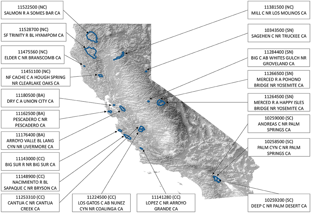
Figure 1. A topographic plot of California and the 20 watershed regions considered in this study.
2.2. LOCA Downscaled Meteorology
For future streamflow projection, the Localized Constructed Analogs (LOCA) dataset (Pierce et al., 2014) is employed. This dataset provides the three necessary input variables for this study, namely precipitation, solar radiation, and near-surface temperature. LOCA is a downscaled dataset ensemble with 6 kilometer resolution over North America from central Mexico through Southern Canada. Among all available LOCA datasets, we downselect four global climate model for this study, which are HadGEM2-ES, CNRM-CM5, CanESM2, and MIROC5 under RCP8.5. These models agree with the four models chosen by California's Climate Action Team Research Working Group as priority models for research contributing to California's Fourth Climate Change Assessment (Pierce et al., 2018). The climatology of these models can be described as warm/dry (HadGEM2-ES), cool/wet (CNRM-CM5), and average (CanESM2). Finally, MIROC5 was selected because it is the most unlike the other three. Since all the basins have irregular shapes, TempestRemap (Ullrich and Taylor, 2015; Ullrich et al., 2016) is used to conservatively regrid the LOCA data to obtain basin-mean forcing data. Because of the uncertainty from both the climate model output and the downscaling process, the historical LOCA data and CAMELS data have some significant disagreements, especially in the values of solar radiation. Specifically, LOCA tends to overestimate the solar radiation compared with NLDAS, as seen in Tables S1–S5. To avoid issues related to this systematic difference, the LOCA data was linearly transformed based on the historical forcing data to match the mean and variance of observations. The same transformation was also applied on the projection forcing data. Specifically, for a given daily input XLOCA, either historical or projection, we denote the transformed value as Xtrans, where μ and σ represent the corresponding mean and standard deviation from the historical period:
The values of μ and σ for NLDAS and the climate model ensemble can be found in Tables S1–S5.
Although LOCA provides historical daily atmospheric forcing data, it is not suitable for model training since it is generated from several climate models via an statistical downscaling method. The climate models produce a simulated climatology which is only constrained to the real world through prescribed atmospheric greenhouse gas concentrations, so there is effectively no relationship between LOCA and observed gage-based streamflow measurements. This is also the reason why we only analyze the climatology of flow rate in section 4, and do not directly compare the time series of streamflow.
2.3. Model Predictors and Target
As mentioned earlier, the input variables (predictors) for our streamflow models are precipitation, temperature, and solar radiation. By default, the input time window size is set it to 365 days (although this is explored later in the text). In general, the length of the input time window needs to be long enough to capture the relevant physical relationships between input variables and streamflow. For each of our ML models, the target variable is streamflow on the last day in the time window. In other words, our objective is to determine the function f in the following equation:
where Q denotes streamflow, P the precipitation, T the temperature, and S the solar radiation. Note that this equation is only provided for the reader to better understand the relationship between streamflow and the independent quantities. The actual functional relationship will vary based on the model architecture. The subscript denotes the corresponding daily value for that particular quantity, and N denotes the input time window size. The input and output variables are all normalized before feeding them into the models via
Here Xi and xi are the ith normalized and original variable, and μ and σ stand for mean and standard deviation of that variable. With the normalized variables having zero mean and unit variance, the specific units and range of the inputs will not influence the model. In turn, the normalization procedure is expected to improve the model performance (e.g., Shanker et al., 1996).
2.4. Machine Learning (ML) Models
Four machine learning model architectures have been investigated and compared with a baseline linear regression model. For the predictive simulations, model performance is quantified by the Nash-Sutcliffe model efficiency (NSE) coefficient (Nash and Sutcliffe, 1970), which is defined as:
where denotes the predicted flow at time t, the observed flow at time t, and the mean observed flow. Here the observed quantities refer to output streamflow from USGS gauge stations. Larger NSE values indicate better performance. Since the NSE is proportional to the square of the difference between model and observations, it tends to put greater emphasis on high flow periods. To maximize NSE, we set 1−NSE as the loss function for our models—that is, the quantity to be minimized during training process. For each model, training is performed separately on each basin but with the same model architecture.
Before training these networks, we first need to set the hyperparameters, which are tuning factors in the model architectures and training process. Common hyperparameters include the number of layers, optimizer, and number of epochs: The number of layers is important to the specific model architecture; the optimizer refers to the gradient descent algorithm used in the training process; and the number of epochs refers to the number of times that the model is trained on the entire training set. The Adam optimizer is used with 0.0005 as the learning rate. We trained each model for 150 epochs with the batch size set to 512. These training configurations are set based on the training loss function, which ensures the loss decreases and stabilizes at a low value. Although the hyperparameters are important for overall model performance (Bergstra and Bengio, 2012), in this work we hold the optimizer and the number of epochs the same for all models. This study does not investigate differences that may arise through more fine tuning of these hyperparameters for specific models—indeed a comprehensive investigation of the optimal hyperparameters for each model is beyond our current computational capability. The remainder of this section describes the architecture of the models investigated in this study.
2.4.1. Linear Regression
Linear regression refers to the simple linear regression model that only incorporates first-order terms from Equation (3). This precludes nonlinear relationships between days in the time series of input variables or between different input variables. As mentioned earlier, the simple linear regression model will be our baseline for assessing the ML models.
2.4.2. Artificial Neural Network (ANN)
An ANN is a traditional neural network composed of dense neural layers (Hassoun et al., 1995). It is an all-connected network without interactions within each single layer. According to the universal approximation theorem, with enough hidden units and depth among the hidden layers, an ANN can simulate any nonlinear relationship (Csáji et al., 2001; Lu et al., 2017). For time series data, however, recurrent neural networks such as GRU and LSTM normally outperform ANNs because of their ability to capture temporal features. In our work, the ANN model has two hidden layers with 100 hidden units and a “ReLU” activation function in each layer. The set of hyperparameters is set based on our coarse tuning for all interested basins. This ANN model is a nonlinear model without temporal features, which is the baseline for the following GRU, LSTM, and CNN models. ANNs have been previously investigated for streamflow prediction in Kisi and Kerem Cigizoglu (2007), and they compared the performance from different ANN models. Noori and Kalin (2016) used an ANN coupled model and it was found that ANN can help improve the streamflow prediction when coupled with physically-based SWAT model.
2.4.3. Gated Recurrent Units (GRU)
As mentioned earlier, recurrent neural networks (RNNs) are typically used to deal with time series and related quantities. However, under simple recurrent designs the gradient will often vanish or explode during the training process (Bengio et al., 1994). As introduced by Cho et al. (2014), GRUs are a typical gated recurrent neural network whose design can help to avoid gradient vanishing for recurrent networks. There are two gates in a GRU cell, referred to as the update gate u and relevant gate r. A general GRU cell is depicted in Figure S1, followed by a set of equations defining the GRU cell. There can be several hidden units in a GRU layer and the number of hidden units is the number of features in cell states.
Similar with the ANN model, a GRU model consists of several layers, with each layer containing several hidden units. In our work, we analyze a three-layer GRU model connected with a dense layer. The GRU layers are set to extract temporal features and the final dense layer is for output. Each GRU layer has 50 hidden units; this number is from coarse hyperparameter searches. The stacked layer design provides sufficient complexity to fit the streamflow data, and provides a similar stacked architecture to compare with the TCNN model.
2.4.4. Long-Short Term Memory (LSTM)
The LSTM model is another example of a gated network, and one which has been increasingly explored in recent years for streamflow forecasting (Kratzert et al., 2019). The primary difference between the LSTM and GRU models is that the LSTM features three gates—the update gate u, the forget gate f and the output gate o. A typical LSTM cell and the corresponding formulas are shown in Figure S2. Like our GRU model, the LSTM model has three LSTM layers and one dense layer. Within each LSTM layer, there are 50 hidden units. The stacked layer design ensures complexity to fit the streamflow data and the same number of cells with GRU can help compare the different model performance.
2.4.5. Temporal Convolutional Neural Network (TCNN)
CNNs remain a widely used model for image processing and analysis because of their ability to extract and decompose features (Gu et al., 2018). The typical input of the CNN model is an image with width, length, and color channels. In our study of streamflow, which is one-dimensional data, the input shape is the number of variables times the input time window size. A typical CNN is comprised of convolutional layers and dense layers. Some CNNs will further add pooling layers between convolutional layers to reduce the dimensionality of the problem and extract important features. But it has also been argued that with sufficiently large convolutional layers, the network can perform well only using convolutional operations (Springenberg et al., 2014). Thus, for simplicity we have only used convolutional layers in our CNN.
A typical CNN architecture used for time-series data is the Temporal Convolutional Neural Network (TCNN) (Lea et al., 2017). Compared with the more well-known CNN for images, TCNNs consist of a one-dimensional network using dilated causal convolutions to keep temporal causation and residual blocks for deeper networks. Bai et al. (2018) tested TCNNs and LSTMs with different time series problems, and argued that TCNNs are better in terms of accuracy and speed for problems of similar complexity. Thus, to compare with our three-layer GRU and LSTM models, we will assess a three-block TCNN with residual connections. Each block has two convolution layers and one residual connection. Dilation rates are set to 1, 6, 12, respectively and kernel size is fixed at 7 for all convolution layers. The number of filters are set to 40, 20, 20 for each block. In the final block, the reception field is large enough to cover the entirety of the time window. Also, with stacked causal convolution blocks, the input information will be concentrated within the last few neurons. To reduce redundancy and avoid overfitting, a slice layer is set after the final TCNN block to only keep last 20 neurons. The TCNN model flow chart and an illustration of dilated causal convolution are shown in Figure S3.
2.5. Ensemble Runs
Unlike the linear model, which has an exact analytical solution, all the neural networks use gradient-based method to optimize the loss function. Since the networks allow for local minima, different initial weights can potentially produce different models with different performance. Thus one needs to be careful to avoid drawing conclusions on the relative performance of each model that are merely a byproduct of the initial weights. In order to eliminate this effect, we run each model 15 times to get an ensemble distribution of NSE values. Thus our results and conclusions are based on the statistical distribution of model performance across the ensemble.
Throughout this study we make use of boxplots for assessing comparative performance between ensembles. As shown in Krzywinski and Altman (2014), comparative performance is intuitive from the boxplot—namely, if the median for one model is above the interquartile range of another, we are confident that it is the better model. However, if the median from the second model lies within the interquartile range of the first model, performance could be the result of randomness in the training process, making it difficult to determine the better model.
3. Results
In this section we first compare the various ML models discussed in section 2.4 to demonstrate the competitive performance of the TCNN. The TCNN is then examined in light of stability under extreme forcing, its sensitivity to choice of input variables across basins, and sensitivity to time window size. A physical interpretation of the observed model sensitivity is also discussed here.
3.1. Model Intercomparison
Figure 2 shows the ensemble prediction results for each basin among the four ML models, plus the linear regression model. The linear regression model performs the worst among available models in almost all basins, in testament to the nonlinearity of the prediction problem. The ANN model tends to achieve a higher NSE value than the linear regression model for almost all basins, but in terms of NSE the ANN is still inferior to the recurrent networks and the TCNN, especially for basins where the NSE values for the recurrent networks and the TCNN are over 0.6, such as 11475560(NC) and 11522500(NC). In these basins, the relatively low NSE scores from the ANN indicate that there are some temporal features that the ANN cannot capture but which are important for streamflow prediction. Nonetheless, for some basins, the ANN outperforms the LSTM. There are two possible reasons this may occur. Firstly, it could be that temporal features are not important for these basins, a hypothesis that is supported by the observation that the ANN tends to also be better than GRU [e.g., basins 11176400(BA) and 11224500(CC)]. On the other hand, the TCNN doesn't have a recurrent architecture so it can effectively ignore the temporal features and mimic the ANN. This could suggest that LSTMs may not be as generalizable as TCNNs. Another possible reason is that the LSTM hyperparameter set is suboptimal for these basins – assessing this possibility may require a more comprehensive basin-dependent hyperparameter search.

Figure 2. Ensemble prediction comparison for all basins with different models. The boxplots denote results over each ensemble of 15 model runs for the ML models. The straight line denotes the linear regression result. For basin 11224500 CC the linear regression model produced a NSE of −2.47.
Among models with temporal features (TCNN, LSTM, GRU), the TCNN exhibits the best average performance. The average NSE over all basins and all ensemble runs is 0.40 for LSTM, 0.44 for GRU, and 0.55 for TCNN. The average NSE value for the best run over all basins is 0.58 for LSTM, 0.58 for GRU, and 0.65 for TCNN. For those basins where LSTM and GRU achieve the highest NSE values, the performance of the TCNN model is competitive—for example, in basins 11141280(CC) and 11284400(SN) the NSE values among the different neural networks are all higher than 0.5. For basins where neural networks do not perform well, such as basins 10259200(SC), 11176400(BA), and 11253310(CC), the TCNN is nonetheless the best among the different neural networks. Notably, the recurrent networks can achieve high NSE values for some basins while performing poorly for other basins. That is, their performance varies substantially among different basins. The TCNN, however, is more stable among all basins: The standard deviation of the ensembles over all basins is 0.47 for LSTM, 0.38 for GRU, and 0.23 for TCNN. Although the choice of hyperparameters is important in these results, the wider spread in the NSE value indicates that for streamflow prediction the recurrent networks have more local minima over the optimization space, and consequently must be trained many times to find a globally optimal configuration.
The stacked recurrent networks here are chosen to compare with the stacked TCNN model. A one-layer LSTM model, such as the one used in Kratzert et al. (2019), is also investigated. We employ 256 hidden units for the LSTM to match (Kratzert et al., 2019). Similarly a one-layer GRU model with 256 hidden units is also compared. With this configuration, the average NSE over all basins and all ensemble runs does improve to 0.47 for the one-layer LSTM, but degrades to 0.34 for the one-layer GRU. The standard deviation is 0.40 and 0.74 for the one-layer LSTM and GRU, respectively. When comparing the average NSE for the best run, the one-layer LSTM and GRU achieve 0.61 and 0.56, respectively. We again tested another one-layer LSTM model with 370 hidden units so as to match the number of free parameters within the TCNN model. The average NSE over all ensemble runs is 0.44, and 0.58 for the best run. The standard deviation is 0.43. A comprehensive comparison can be found in Table 1. Figure S4 shows the ensemble prediction comparison of the TCNN model with one-layer recurrent networks. Compared with the one-layer recurrent networks, the TCNN model still exhibits slightly better performance with lower variation.

Table 1. Mean and standard deviation for ensemble prediction comparison with different models.
Besides evaluating the NSE value for the whole prediction period, we also examined the model performance for high flow and low flow days. High flow (low flow) days are defined as days when the observed flow rate is higher (lower) than the 95th (5th) percentile over all days. Since the low flow series for some basins is zero throughout, NSE cannot be used to assess performance. Instead, we use mean squared error (MSE) to quantify the performance, given by
The MSE spread for all basins over the ensemble can be found in Figures S5, S6. Whereas the TCNN tends to perform well during high flow periods, the LSTM does exhibit better performance in low flow periods. For the high flow period, when average MSE is compared over all the ensemble runs, the TCNN achieves the best performance on 12 basins compared with 4 basins for LSTM. When comparing the minimum MSE for the high flow period, the TCNN is the best model for 10 basins compared with 6 basins for LSTM. For the low flow period, when using the average MSE, TCNN is the best model for 2 basins compared with 10 basins for LSTM; when assessing minimum MSE value, the LSTM is superior in 16 basins. The reason for this behavior is likely a simple consequence of the chosen hyperparameters of the model; further optimization will likely result in incremental improvements to both the TCNN and LSTM. Notably, the purpose for the comparisons in this section are not to show the TCNN is better than the LSTM, since such a proof would require us to effectively test all possible architectures and hyperparameters. Instead, these results demonstrate that the TCNN can achieve comparable performance to other commonly used models.
In addition to assessing model performance, training time also merits comparison among the different models. The average training time for one basin with the ANN on a single RTX 2080Ti is 11 s, 77 s for TCNN, 149 s for stacked GRU, and 150 s for stacked LSTM. For the one-layer LSTM model, it takes 220 s for 256 hidden units and 380 s for 370 hidden units. Hence, for this particular configuration the TCNN model is the fastest among the models with temporal features, although only by a factor of two.
Based on the results presented in this section, TCNN is chosen as our candidate network for prediction and projection of streamflow. The remainder of this paper now focuses assessing and explaining the performance of the TCNN.
3.2. Model Stability Under Extreme Climatological Forcing
One of the biggest challenges for ML projection is concept drift (also known as non-stationarity). Under climate change, it is widely accepted that the statistical properties of the input predictors and output streamflow will change through time. Although surface temperatures are expected to increase almost everywhere, in parts of California these increases are also accompanied by an increase in total precipitation of about 1.2% per decade (Ullrich et al., 2018). It is further expected that the input variance will increase in conjunction with more frequent extreme precipitation and temperature events (Swain et al., 2018). However, because the TCNN model is trained on historical data, the end-of-century inputs may incur extrapolation, which has the potential to produce unphysical results such as negative flow. To test whether the TCNN model is able to produce physically reasonable results even when inputs are not within the range of the training data, an idealized test is devised to stress the model far beyond the long-term range of possible inputs. Specifically, the model was executed with quadruple precipitation and a temperature increase of 5 degrees Celsius from the training set. Only one simulation was performed for each basin, using the TCNN model with highest NSE value from the ensemble run.
The extreme scenario investigated here is unrealistic even in light of climate change. However, if the ML model were not stable, this extreme scenario, far outside the realm of the training data, should cause the model to “blow up” or generate negative flow rates. However, if our model can still produce acceptable results under such an extreme scenario, we have greater confidence that it will generate reasonable projection results under the RCP8.5 scenario. Results from a single representative basin are depicted in Figure 3. Although only one basin in shown here, the results are analogous in other basins (not shown). As expected, the projected streamflow is generally much larger than historical, with much higher flood peaks. In addition, the high flow period is longer under this test as a result of precipitation accumulation, and low flow periods produce consistently higher streamflow. The regression line from the scatter plot is Qp = 4.001 × Qh (R2 = 0.74), where Qp is projection streamflow and Qh is the historical streamflow. Thus the 4× increase in precipitation produces approximately a 4× increase in streamflow. However, this simple linear factor appears to underestimate flows on the low flow days and overestimate flows during high flow days, again indicative of nonlinearity in the streamflow dynamics.
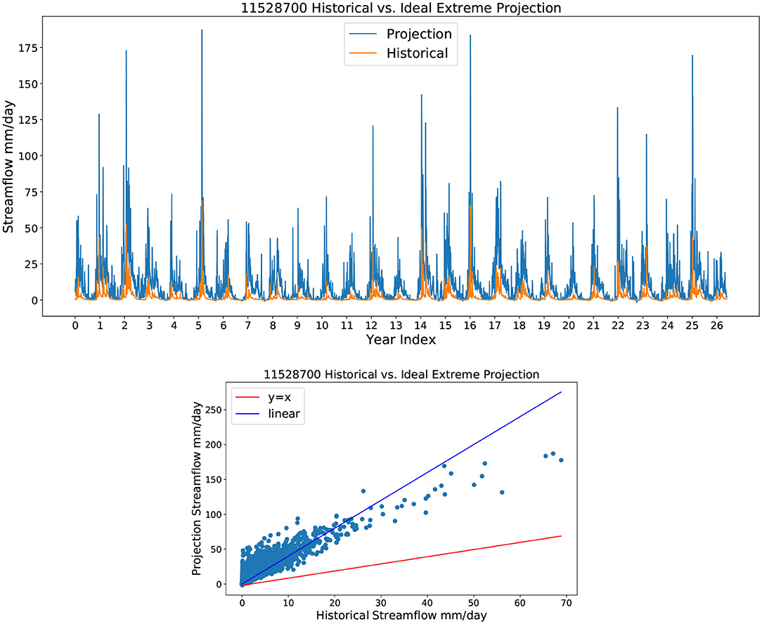
Figure 3. A depiction of the streamflow response under idealized extreme forcing showing (top) time series of flow and (bottom) historical streamflow vs. projected streamflow.
3.3. Model Sensitivity to Input Variables
As discussed earlier, the input variables for our full model are precipitation, temperature, and solar radiation. Although input fields beyond precipitation can improve model performance by capturing significant physical relationships, they also increase the complexity of the model, potentially leading to a wider spread among trained models. To test the importance of these variables for streamflow prediction three reduced models were compared, consisting of precipitation solely (p), precipitation and temperature (pt), and precipitation and solar radiation (ps). When comparing the performance of reduced models and the full model, the 15-model ensemble was again used to avoid noise from the initial state.
The overall performance of ps and pt models is again assessed using box plots of NSE values. Figure 4 shows the result of the ensemble comparison. It is apparent that for some basins temperature boosts predictability, while for others solar radiation is more important. There are only three basins where the best pst model is better than the best ps or pt model [11264500(SN), 11266500(SN), and 11381500(NC)], and in each of these cases the improvement with all three variables is modest. In each basin, the dominant variable does reflect the geographic features of the basin. Basins where temperature significantly improves performance are 10343500 (SN), 11264500 (SN), 11266500 (SN), 11451100 (NC), 11522500 (NC), 11176400 (BA), and 11224500 (CC) which include three Sierra Nevada basins, two Northern California basins, and one Bay Area basin. Basins where solar radiation improves performance are 10258500 (SC), 10259000 (SC), 11143000 (CC), 11253310 (CC), 11180500 (BA), 11284400 (SN), and 11475560 (NC)—except for the last two, these are located in coastal areas or in the inland desert of Southern California. These results suggest that, to a close approximately, we can divide the basins into three categories using these reduced models: those where temperature is important (generally in mountainous regions), those where solar radiation is important (generally near coastlines), and those where temperature and solar radiation offer no significant benefit to predictability.
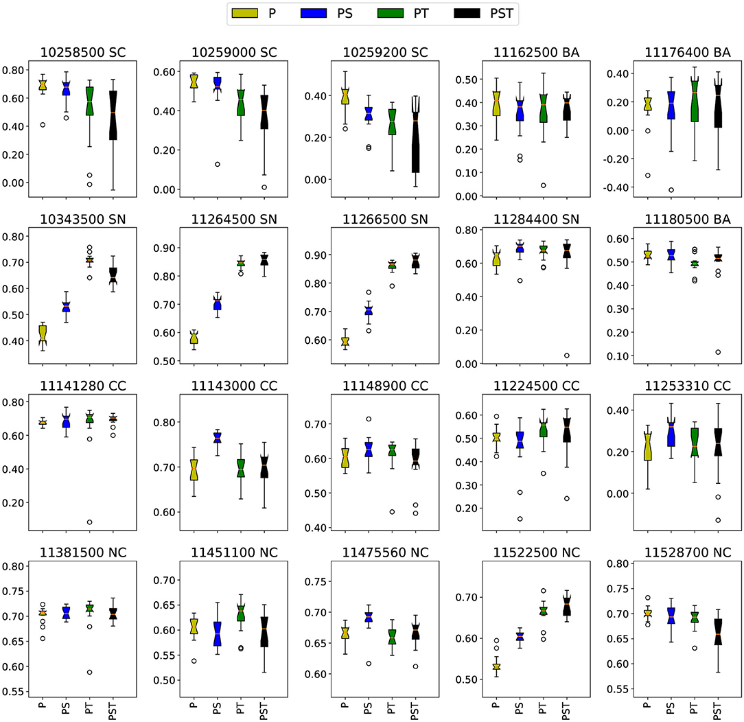
Figure 4. Ensemble prediction comparison for all basins with different reduced TCNN models.
The physical explanation underlying the performance of the reduced models is related to the climatological properties of these different basins. For instance, in the basins of the Sierra Nevadas and Northern California, accumulation and melt of wintertime snowpack generally plays an important role in driving streamflow. However, the inclusion of temperature in these mountainous regions does not necessarily guarantee a performance improvement. For instance, temperature does not improve the model of 11528700 (NC), where snow is a major driver for streamflow; nonetheless, the inclusion of temperature also does not significantly degrade performance. Further, in basins where temperature improves performance we also generally see that inclusion of solar radiation does provide some improvement over the models only using precipitation—this suggests that the ML model is potentially identifying the relationship between solar radiation and temperature, or is instead using solar radiation to estimate snow melt rates.
The physical processes driving streamflow in the coastal basins are significantly different than those of the mountains. Namely, coastal basins do not experience significant temperature variations as a result of temperature regulation by the ocean. Further, because the ocean provides a ready source of moisture, air remains close to saturation. In accordance with the Penman-Monteith equation, evaporation from these basins will be driven primarily by radiative forcing, in agreement with our results. Among the central coast basins, the one exception that shows improved performance with temperature, but no significant improvement from solar radiation is 11224500 (CC). Although this basin is on the Central Coast, it is far from the coastline and so subject to larger temperature swings and lower relative humidity. The relatively high-altitude coastal ranges in this basin do produce occasional snow accumulation, but it is unlikely that snow dynamics plays a role here.
For those basins where inclusion of solar radiation and temperature produce worse model performance (i.e., the three Southern California basins), we hypothesize that the ML model is either identifying non-existent physical relationships between these variables and streamflow in the training data, or that the increased model complexity is making it more difficult for the model to converge to an optimal configuration. The truth is likely a combination of both of these factors, as for all three SC basins the “best performing” pst model is not significantly worse than the median p-only model, but is clearly worse than the best p-only model.
In conclusion, the reduced models explored here are helpful for giving insight into the processes that are most relevant for each basin, and thus the relevant causative relationships. Here snowpack dynamics and coastal meteorology have emerged as two obvious geographical features important for determining model behavior. Given this behavior agrees with our physical understanding of the system, we have further evidence to suggest that the models are behaving credibly.
3.4. Model Sensitivity to Time Window Size
The input time window size is an important hyperparameter for our model, and one that is intrinsically connected to the physical processes driving streamflow. However, a time window that is too large can reduce model performance and slow training time. Some past studies set the time window size based on the results from a purely statistical analysis of autocorrelation or partial correlation (Yaseen et al., 2016; Peng et al., 2017). In this study, we estimate the time window size from an understanding of the physical properties of each region. For streamflow prediction and projection, the response time for precipitation, groundwater and snowpack can range from several hours to months, and a proper time window size should capture all necessary features and avoid redundant information. The seasonality of the streamflow varies regionally and depends on the climatic characteristics and the contribution of snow/ice, and anthropologenic interventions. An investigation of monthly global steamflow (Dettinger and Diaz, 2000) indicated that lags between the peak precipitation and peak steamflow peaks up to 11 months, while 0–3 months was the typical value. In this study we explore 100, 180, and 365 days as different window sizes. The 365-day window corresponds to an entire water year, and so should capture all potential physical processes except for long-term withdrawals or variations in groundwater. The 100-day window captures a typical season length and the 180-day window is in between these two. Figure 5 shows the ensemble performance results comparing models with different time window sizes.
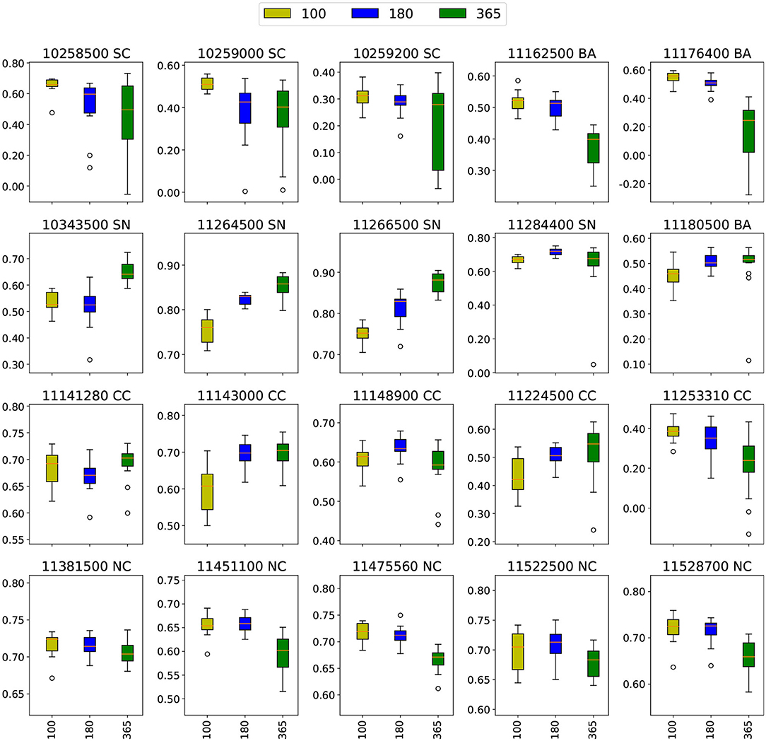
Figure 5. Ensemble prediction comparison for all basins with different window sizes.
What stands out in Figure 5 is the monotonic tendencies in most basins. There are increasing tendencies with the time window size for basins 11224500 (CC), 10343500 (SN), 11264500 (SN), and 11266500 (SN), while 11162500 (BA), 11176400 (BA), 11253310 (CC), 11475560 (NC), and 11528700 (NC) show decreasing tendencies. An increasing tendency implies the presence of slow processes governing streamflow, whereas a decreasing tendency implies upstream processes are fast and there is no significant benefit in using a larger window size. In fact, we can again classify basins into two categories by their monotonic tendencies. Similar with the previous interpretation of different predictors, these results are likely to be related to physical factors, especially snowpack—particularly because of its long response time. In general, the basins with increasing tendencies are in mountainous area like Sierra Nevada and the Coastal Ranges while basins with decreasing tendencies are in Northern California, the Bay Area, and the Central Coast, which are closer to the Pacific. Mountainous areas tend to have more snowpack due to their higher elevation and thus streamflow there is more likely influenced by snowpack. For coastal areas, snowpack does not play a role in streamflow dynamics, and since the temperature is more stable relative to inland areas, the impact from snowpack will also be weaker than that in inland basins. Therefore, snowpack should be the primary factor driving the direction of the tendency. Another factor not explored here that may affect the tendency is the groundwater response time—this may play a role in central coast basins such as 11143000 (CC) and 11224500 (CC), which respond positively to increased time window size.
4. Projected Streamflow
The best models from the ensemble run for each basin are now employed with remapped and rescaled LOCA data to produce our projection dataset. As described in section 2.2, we first apply TempestRemap to obtain mean forcing data for irregular basins from the gridded LOCA product. Then both future and historical forcing from LOCA are rescaled (bias corrected) based on the historical observations before being used to drive the ML model. Tables S6–S8 show the mean daily precipitation, temperature and solar radiation from NLDAS and the four climate models employed. Figures S7–S9 also show the climatological daily mean of these variables. Generally CanESM2, CNRMCM5, and HadGEM2ES suggest a future wetter climate with more precipitation, while MIROC5 tends to produce similar or less precipitation for these basins. Essentially all the basins are projected to experience higher daily temperatures, but the change in solar radiation is small. Figures 6, 7 show climatological daily streamflow with historical and under the future projection with RCP8.5 forcing. The daily streamflow projection dataset produced in this manner is available at Duan et al. (2020) with the units of millimeters per day. Within the database, each file has the name as the format of “nnnnnnnn-model-scenario.csv.” The first eight digits are HUC8 identifiers for each basin, followed by the climate model name, and then the scenario (either “hist” or “RCP8.5”).
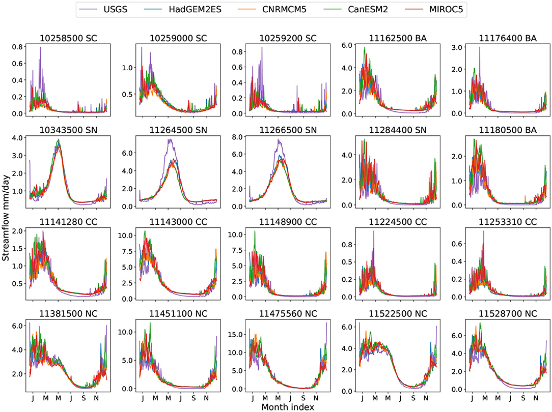
Figure 6. Historical climatological daily streamflow from USGS and four climate models.
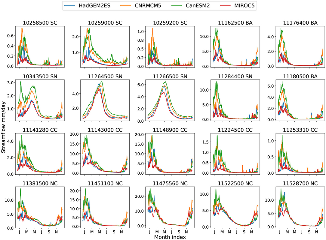
Figure 7. Projection climatological daily streamflow from four climate models.
4.1. Analysis of the Projected Streamflow
Since the historical forcing from different climate models are corrected to match observations (as discussed in section 2.2), historical streamflow exhibits nearly the same pattern and magnitude with forcings from different climate models (Figure 6). Compared with USGS observation, the flows tend to match fairly well except in a few SC and SN basins, where a clear magnitude difference at the flow peak emerges. For 10258500(SC) and 10259200(SC), even with the NLDAS forcing data the TCNN underestimates the peak, so we can conclude that the TCNN simply does not identify a relationship between forcing and streamflow during these high flow events. Looking at the SN basins, Figure 2 shows that the TCNN model achieves an NSE score around 0.9 for 11264500(SN) and 11266500(SN), so in this case the differences are likely due to differences between the forcing from NLDAS vs. LOCA. Namely, we can deduce that for these basins the Gaussian bias correction (2) still produces a forcing which is still somewhat inconsistent with historical forcing. For 11264500(SN) and 11266500(SN) the primary source of this error appears to be wintertime and springtime temperatures, which are intimately connected to precipitation phase and snowpack melt rate; when the LOCA temperatures and radiation are replaced with NLDAS temperatures and radiation (while retaining the LOCA precipitation) the correct streamflow curves are recovered (Figure S13).
To assess the magnitude of future change, we examine the projected flow duration curve (FDC) vs. the historical FDC from the same climate model. Figure 8, Figures S14–S16 show the projected future and historical FDCs with four different climate models. When the projected streamflow curve is above the historical curve, the ML model indicates that higher streamflow rates become more probable. It is perhaps not surprising that since precipitation increases across almost all basins, almost all of the basins show increasing streamflow. The projections also generally indicate that the peak flow rate will be higher, potentially indicative of an increased probability of flooding (although the degree to which this is possible is a subject for future investigation). Note that the multimodel CMIP5 ensemble does produce some disagreement: For instance, under the MIROC5 projection, the FDC curves for historical and projection match closely for the most basins. As noted earlier, the MIROC5 model is considered the most unlike the other CMIP5 models in this investigation, tending to produce precipitation amounts that are relatively constant over time.
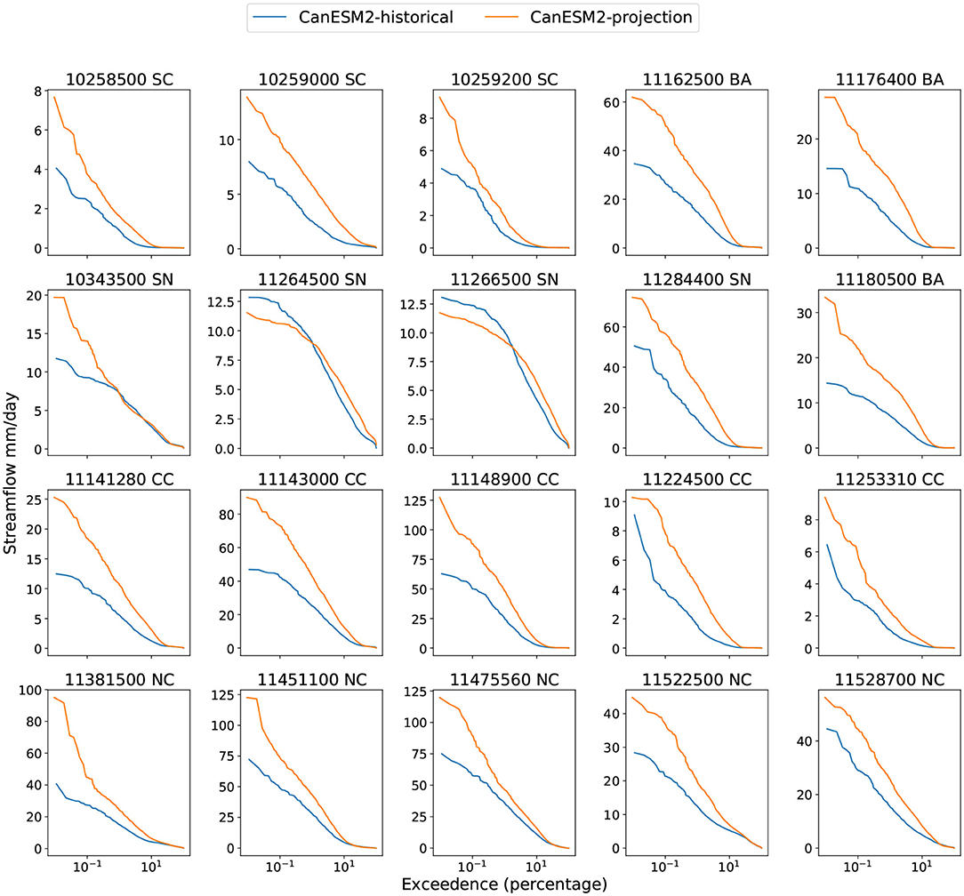
Figure 8. Flow duration curve with CanESM2 forcing over both historical and future (projection) periods.
Although most basins see an increase in flow rate, basins 10343500 (SN), 11264500 (SN), and 11266500 (SN) are notable exceptions. For these three basins, the future FDC curves are sometimes below the historical curves (this is even more obvious with MIROC5 forcing). For basins 11264500 (SN) and 1266500 (SN) lower flow rates become more probable but the maximum flow rate decreases. These three basins are all in the Sierra Nevada area—10343500 (SN) in the Tahoe National Forest and the other two in Yosemite. Examining Figures 6, 7, these three basins exhibit significant differences in the character of their flow compared with other basins. Namely, the climatological streamflow for these basins shows a peak in late Spring and Summer, while other basins are peaked in the winter season. Since we have shown earlier that streamflow in these basins are driven by snow dynamics, differences in streamflow are likely due to the impact of a slow snowmelt process. Notably, this is in accord with our previous discussion in sections 3.3, 3.4, where these basins are temperature dominant and benefit from longer time window sizes. These projection results lend further evidence to the claim that streamflow in these basins is highly dependent on snowmelt.
The change in the peak flow timing for each basin was also investigated. The peak time is defined as the day of maximal flow rate for the year, measured in days since the beginning of a water year (set to October 1st in our study). Figure 9 shows the peak time for each basin in historical and projection years with MIROC5 forcing. Peak timing figures with forcings from other climate models can be found in Figures S17–S19. Although there is generally no significant change in peak timing for most basins, the Sierra Nevada basins are again outliers. Namely, there is a statistically significant shift to earlier peak times in these snowpack-dominated basins. Although it is not always the case for all the climate models, the projected lead of peak time associated with decrease of streamflow in the future again captures the unique hydrology dynamics in the Sierra Nevadas.
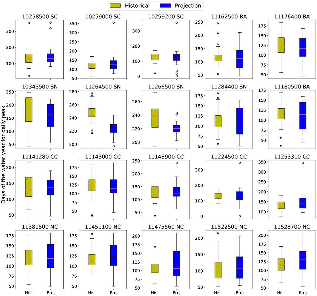
Figure 9. Day of peak flow for each basin with MIROC5 forcing.
4.2. Understanding Nonlinearity in the Projection
To better understand the nonlinearity of the streamflow response to forcing under climate change, we consider a decomposition of the response according to its predictors. Specifically, the impact of precipitation alone on the projected streamflow can be isolated by holding the temperature and solar radiation at historical values while using the future projected precipitation. An analogous approach can then be employed for temperature and solar radiation. By then subtracting the historical streamflow time series from each of these streamflow projections, we obtain ΔQp, ΔQt, ΔQs, the change in streamflow from precipitation alone, temperature alone, and solar radiation alone. These are contrasted against ΔQpts, which denotes the change in streamflow from all three factors. From the first-order Taylor series expansion we then have
for some residual r that captures the influence of high-order terms. The linear response is defined as summation of three individual responses. To reduce noise from daily variations in streamflow, the monthly averaged streamflow is used for comparison. In Figure 10, we plot ΔQpts vs. ΔQlinear, with the R2 value in the title. A fully linear response would be expected to lay along the y = x line.
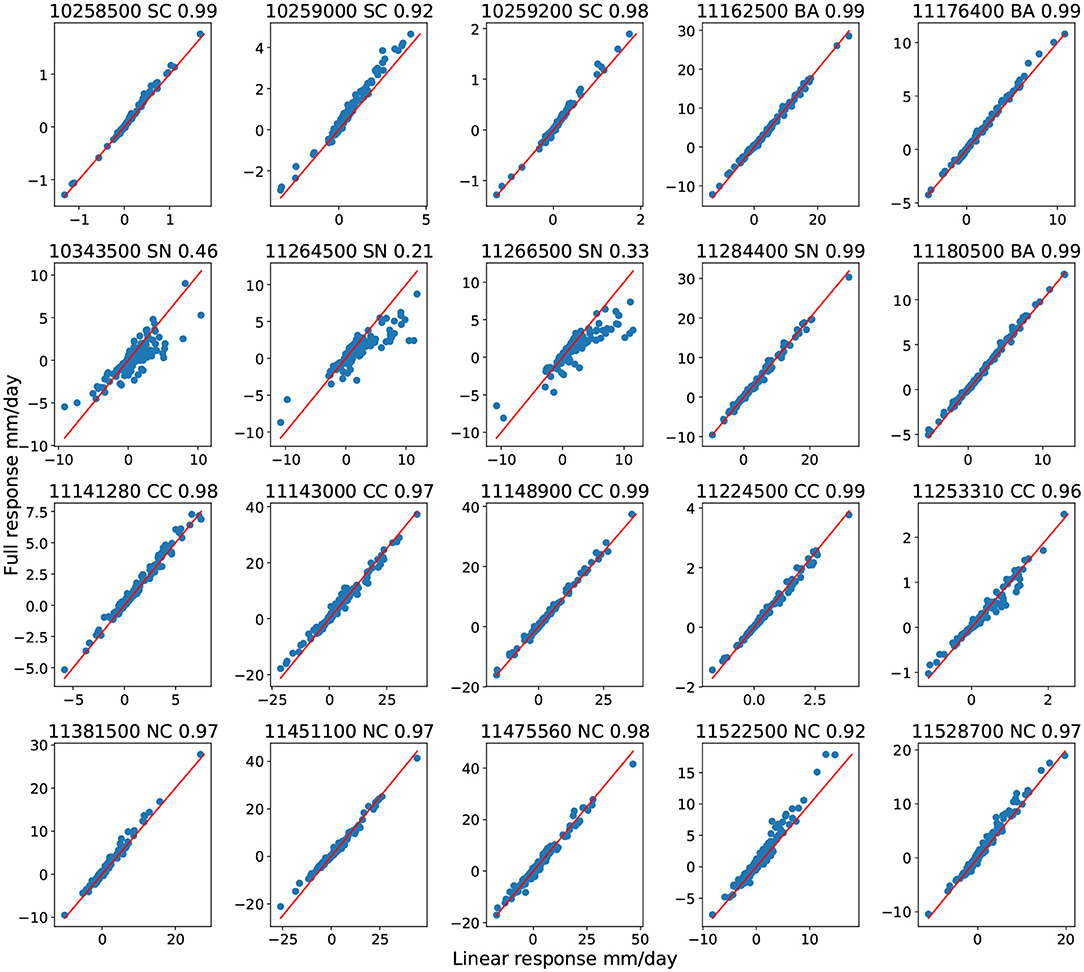
Figure 10. Full response and linear response for all basins with CanESM2 forcing.
As seen in Figure 10, almost all basins show a nearly linear response to the input variables, except for basin 10343500(SN), 11264500 (SN), and 11266400(SN)—all in the Sierra Nevada mountains. From our discussion in sections 3.3, 3.4, these SN basins are temperature dominated and require a longer time window size to correctly capture streamflow, indicating the interplay between precipitation and temperature in governing snow processes.
5. Conclusions and Future Work
In this study, we have designed and analyzed a general temporal convolutional neural network for streamflow projection in California. Causal convolution is used to maintain physical causation. The input consists of precipitation, temperature, and solar radiation over a particular past window size. In prediction mode, the TCNN model is compared with other commonly used ML models based on ensemble performance so as to eliminate random effects from initializing the training. The results of this intercomparison indicate there are some important temporal features that ANNs struggle to capture, in contrast to TCNNs and other recurrent neural networks (LSTMs and GRUs). Compared with other recurrent networks, the TCNN model is faster and more stable under training. Overall, the TCNN produces better agreement both on average and in the high-flow regime, whereas the LSTM was better in the low-flow regime. Like these other networks, the TCNN model can also be generalized to other basins while maintaining the same architecture.
To demonstrate model stability under extreme forcing, an idealized test with quadruple precipitation and 5 Celsius higher temperature is implemented to verify whether the model produces reasonable results when tested with data outside the training regime. A qualitative analysis and linear regression of projected streamflow against historical precipitation suggests our model produces physically acceptable results for projection.
We have also observed that the TCNN model can build different functional relationships for different basins, as demonstrated through the examination of reduced models, models with different time window sizes, and the nonlinear response of the model to input variables. With this understanding of the “under the hood” workings of the ML model, we can distinguish different geographic features across basins. This classification ability suggests our model can simulate physical processes with causal convolution as a constraint. In regions where snowpack is relevant, we conclude that temperature should be included as a model covariate; whereas in coastal regions, solar radiation should be included. Including both variables was not observed to significantly improve model performance in any basin. Also, in regions where snowpack is relevant, a longer time window size is desirable for model performance (here we tested a 365-day window), whereas in other regions a shorter time window of 100-days produced better results.
Under the RCP8.5 scenario, the nonlinearity of the streamflow response was examined by decomposing the response into three modes by the predictors. By inspecting the linear response and full response, we observed that most basins exhibit a linear response from precipitation, temperature, and solar radiation, except for the basins in Sierra Nevada. The nonlinearity is likely associated with snowpack, which is a physical feature that is sensitive to both precipitation and temperature.
Model results for future projections and historical hindcasts were compared to understand the changing character of the streamflow. Generally streamflow in most basins increases through the end of the century, except for the Sierra Nevada basins. Peak flow time remained statistically indistinguishable among most basins, except the Sierra Nevada basins which showed a shift to earlier dates under some models. These results further indicate that the snow dynamics in the Sierra Nevada is important for correctly capturing streamflow in these basins.
The idealized test here mainly deals with the problem of model stability under extrapolation. In terms of ensuring the model produces physically plausible results under extreme forcings, we need to compare with a physically based model with the same extreme forcing. This problem has been saved for our future work. Also, to better understand the ML model and ensure its credibility for producing future projections, we intend to next cross-validate our projection datasets with a physically-based model over the same time period. Model credibility can also be enhanced through alternative designs that explicitly include physically-based conservation laws. For instance, subsurface flow or evaporation are not produced as outputs, and so validation of the water budget is impossible. With a more complicated design, ML models could predict streamflow, evaporation and groundwater, and be constrained via an appropriate physically-based conservation law. Such constraints would further enable physical interpretation of the model results. Finally, we wish to determine if the TCNN can be used to interpolate predictors to higher temporal resolution, for use (for instance) in physically-based models. The ML model could also be used to examine model performance when the strict causation is relaxed (namely, if future streamflow could provide a better estimate of present streamflow).
Data Availability Statement
The datasets presented in this study can be found in online repositories. The names of the repository/repositories and accession number(s) can be found in the article/Supplementary Material.
Author Contributions
SD, PU, and LS designed the model. SD and PU designed the experiments and wrote the manuscript. SD carried out the experiments. All authors contributed to the article and approved the submitted version.
Funding
This work was supported by California Energy Commission grant Advanced Statistical-Dynamical Downscaling Methods and Products for California Electrical System project (award no. EPC-16-063) and the U.S. Department of Energy Regional and Global Climate Modeling Program (RGCM) An Integrated Evaluation of the Simulated Hydroclimate System of the Continental US project (award no. DE-SC0016605).
Conflict of Interest
The authors declare that the research was conducted in the absence of any commercial or financial relationships that could be construed as a potential conflict of interest.
Acknowledgments
We wish to thank David Pierce and Sam Iacobellis for their help with LOCA dataset and Andrew Newman for his help with CAMELS dataset. We would like to thank MetroIT in UC Davis for the help with the GPU cluster.
Supplementary Material
The Supplementary Material for this article can be found online at: https://www.frontiersin.org/articles/10.3389/frwa.2020.00028/full#supplementary-material
References
Atieh, M., Taylor, G., Sattar, A. M., and Gharabaghi, B. (2017). Prediction of flow duration curves for ungauged basins. J. Hydrol. 545, 383–394. doi: 10.1016/j.jhydrol.2016.12.048
Bai, S., Kolter, J. Z., and Koltun, V. (2018). An empirical evaluation of generic convolutional and recurrent networks for sequence modeling. arXiv preprint arXiv:1803.01271.
Bengio, Y., Simard, P., and Frasconi, P. (1994). Learning long-term dependencies with gradient descent is difficult. IEEE Trans. Neural Netw. 5, 157–166. doi: 10.1109/72.279181
Bergstra, J., and Bengio, Y. (2012). Random search for hyper-parameter optimization. J. Mach. Learn. Res. 13, 281–305.
Cho, K., Van Merriënboer, B., Gulcehre, C., Bahdanau, D., Bougares, F., Schwenk, H., et al. (2014). Learning phrase representations using RNN encoder-decoder for statistical machine translation. arXiv preprint arXiv:1406.1078. doi: 10.3115/v1/D14-1179
Csáji, B. C. et al. (2001). Approximation With Artificial Neural Networks. Faculty of Sciences, Etvs Lornd University, Hungary.
Dettinger, M. D., and Diaz, H. F. (2000). Global characteristics of stream flow seasonality and variability. J. Hydrometeorol. 1, 289–310. doi: 10.1175/1525-7541(2000)001<0289:GCOSFS>2.0.CO;2
Duan, S., Ullrich, P., and Shu, L. (2020). California streamflow projection dataset. Zenodo. doi: 10.5281/zenodo.3823273
Feng, D., Fang, K., and Shen, C. (2019). Enhancing streamflow forecast and extracting insights using long-short term memory networks with data integration at continental scales. arXiv preprint arXiv:1912.08949. doi: 10.1029/2019WR026793
Gao, C., Gemmer, M., Zeng, X., Liu, B., Su, B., and Wen, Y. (2010). Projected streamflow in the Huaihe river basin (2010-2100) using artificial neural network. Stochast. Environ. Res. Risk Assess. 24, 685–697. doi: 10.1007/s00477-009-0355-6
Gu, J., Wang, Z., Kuen, J., Ma, L., Shahroudy, A., Shuai, B., et al. (2018). Recent advances in convolutional neural networks. Pattern Recogn. 77,354–377. doi: 10.1016/j.patcog.2017.10.013
Huang, S., Chang, J., Huang, Q., and Chen, Y. (2014). Monthly streamflow prediction using modified emd-based support vector machine. J. Hydrol. 511, 764–775. doi: 10.1016/j.jhydrol.2014.01.062
Huang, X., and Ullrich, P. A. (2017). The changing character of twenty-first-century precipitation over the western united states in the variable-resolution CESM. J. Clim. 30, 7555–7575. doi: 10.1175/JCLI-D-16-0673.1
Kisi, O., and Cimen, M. (2011). A wavelet-support vector machine conjunction model for monthly streamflow forecasting. J. Hydrol. 399, 132–140. doi: 10.1016/j.jhydrol.2010.12.041
Kisi, O., and Kerem Cigizoglu, H. (2007). Comparison of different ANN techniques in river flow prediction. Civil Eng. Environ. Syst. 24, 211–231. doi: 10.1080/10286600600888565
Koirala, S., Hirabayashi, Y., Mahendran, R., and Kanae, S. (2014). Global assessment of agreement among streamflow projections using CMIP5 model outputs. Environ. Res. Lett. 9:064017. doi: 10.1088/1748-9326/9/6/064017
Kratzert, F., Klotz, D., Shalev, G., Klambauer, G., Hochreiter, S., and Nearing, G. (2019). Benchmarking a catchment-aware long short-term memory network (LSTM) for large-scale hydrological modeling. arXiv preprint arXiv:1907.08456. doi: 10.5194/hess-2019-368
Krzywinski, M., and Altman, N. (2014). Visualizing samples with box plots: use box plots to illustrate the spread and differences of samples. Nat. Methods 11, 119–121. doi: 10.1038/nmeth.2813
Le, X.-H., Ho, H. V., Lee, G., and Jung, S. (2019). Application of long short-term memory (LSTM) neural network for flood forecasting. Water 11:1387. doi: 10.3390/w11071387
Lea, C., Flynn, M. D., Vidal, R., Reiter, A., and Hager, G. D. (2017). “Temporal convolutional networks for action segmentation and detection,” in Proceedings of the IEEE Conference on Computer Vision and Pattern Recognition (Honolulu, HI), 156–165. doi: 10.1109/CVPR.2017.113
Lu, Z., Pu, H., Wang, F., Hu, Z., and Wang, L. (2017). “The expressive power of neural networks: a view from the width,” in Advances in Neural Information Processing Systems (Long Beach, CA), 6231–6239.
Nash, J. E., and Sutcliffe, J. V. (1970). River flow forecasting through conceptual models part I-a discussion of principles. J. Hydrol. 10, 282–290. doi: 10.1016/0022-1694(70)90255-6
Newman, A., Sampson, K., Clark, M., Bock, A., Viger, R., and Blodgett, D. (2014). A large-sample watershed-scale hydrometeorological dataset for the contiguous USA. Boulder, CO: UCAR/NCAR.
Noori, N., and Kalin, L. (2016). Coupling swat and ann models for enhanced daily streamflow prediction. J. Hydrol. 533, 141–151. doi: 10.1016/j.jhydrol.2015.11.050
Peng, T., Zhou, J., Zhang, C., and Fu, W. (2017). Streamflow forecasting using empirical wavelet transform and artificial neural networks. Water 9:406. doi: 10.3390/w9060406
Pierce, D. W., Cayan, D. R., and Thrasher, B. L. (2014). Statistical downscaling using localized constructed analogs (loca). J. Hydrometeorol. 15, 2558–2585. doi: 10.1175/JHM-D-14-0082.1
Pierce, D. W., Kalansky, J. F., and Cayan, D. R. (2018). Climate, drought, and sea level rise scenarios for California's fourth climate change assessment. Technical report, Technical Report CCCA4-CEC-2018-006, California Energy Commission.
Rasouli, K., Hsieh, W. W., and Cannon, A. J. (2012). Daily streamflow forecasting by machine learning methods with weather and climate inputs. J. Hydrol. 414, 284–293. doi: 10.1016/j.jhydrol.2011.10.039
Shanker, M., Hu, M. Y., and Hung, M. S. (1996). Effect of data standardization on neural network training. Omega 24, 385–397. doi: 10.1016/0305-0483(96)00010-2
Shen, C. (2018). A transdisciplinary review of deep learning research and its relevance for water resources scientists. Water Resour. Res. 54, 8558–8593. doi: 10.1029/2018WR022643
Springenberg, J. T., Dosovitskiy, A., Brox, T., and Riedmiller, M. (2014). Striving for simplicity: the all convolutional net. arXiv preprint arXiv:1412.6806.
Swain, D. L., Langenbrunner, B., Neelin, J. D., and Hall, A. (2018). Increasing precipitation volatility in twenty-first-century California. Nat. Clim. Change 8, 427–433. doi: 10.1038/s41558-018-0140-y
Tsymbal, A. (2004). The Problem of Concept Drift: Definitions and Related Work. Computer Science Department, Trinity College Dublin.
Ullrich, P. A., Devendran, D., and Johansen, H. (2016). Arbitrary-order conservative and consistent remapping and a theory of linear maps: Part II. Mon. Weather Rev. 144, 1529–1549. doi: 10.1175/MWR-D-15-0301.1
Ullrich, P. A., and Taylor, M. A. (2015). Arbitrary-order conservative and consistent remapping and a theory of linear maps: Part I. Mon. Weather Rev. 143, 2419–2440. doi: 10.1175/MWR-D-14-00343.1
Ullrich, P. A., Xu, Z., Rhoades, A. M., Dettinger, M. D., Mount, J. F., Jones, A. D., et al. (2018). California's drought of the future: a midcentury recreation of the exceptional conditions of 2012-2017. Earth's Fut. 6, 1568–1587. doi: 10.1029/2018EF001007
White, A. B., Moore, B. J., Gottas, D. J., and Neiman, P. J. (2019). Winter storm conditions leading to excessive runoff above California's Oroville Dam during January and February 2017. Bull. Am. Meteorol. Soc. 100, 55–70. doi: 10.1175/BAMS-D-18-0091.1
Yan, L., Feng, J., and Hang, T. (2019). “Small watershed stream-flow forecasting based on LSTM,” in International Conference on Ubiquitous Information Management and Communication (Phuket: Springer), 1006–1014. doi: 10.1007/978-3-030-19063-7_79
Keywords: machine learning, temporal convolutional neural network, model sensitivity, streamflow projection, projection analysis
Citation: Duan S, Ullrich P and Shu L (2020) Using Convolutional Neural Networks for Streamflow Projection in California. Front. Water 2:28. doi: 10.3389/frwa.2020.00028
Received: 14 May 2020; Accepted: 04 August 2020;
Published: 16 September 2020.
Edited by:
Chaopeng Shen, Pennsylvania State University (PSU), United StatesReviewed by:
Jie Niu, Jinan University, ChinaKuai Fang, Pennsylvania State University (PSU), United States
Copyright © 2020 Duan, Ullrich and Shu. This is an open-access article distributed under the terms of the Creative Commons Attribution License (CC BY). The use, distribution or reproduction in other forums is permitted, provided the original author(s) and the copyright owner(s) are credited and that the original publication in this journal is cited, in accordance with accepted academic practice. No use, distribution or reproduction is permitted which does not comply with these terms.
*Correspondence: Shiheng Duan, c2hpZHVhbkB1Y2RhdmlzLmVkdQ==