Integrating Invasive and Non-invasive Monitoring Sensors to Detect Field-Scale Soil Hydrological Behavior

In recent decades, while great emphasis has been given to the monitoring of point-scale soil moisture patterns and field-scale integrated soil moisture, the measurement of matric potential has attracted little attention. Information on the soil matric potential is available in point-scale measurements but is still missing at field-scale. This state variable is necessary to understand hydrological fluxes and to determine the soil water retention function (WRF) for field-scale applications. In this study, we combine data from cosmic-ray neutron probes (CRNP, non-invasive proximal soil moisture sensors) and SoilNet wireless sensor networks (invasive ground-based soil moisture and matric potential sensors) installed in two sub-catchments with contrasting land-use (agroforestry vs. near-natural forest) to derive a field-scale WRF. We investigate the hypothesis that both sensor types provide effective measurements that are representative for the entire sub-catchment, as well as the drawbacks of integrating the different measurement scales of the sensor types (i.e., spatial-mean of distributed point-scale data vs. an integrated field-scale measurement). We found discrepancies in the data of the two sensor types related to the effects of the time-varying vertical measurement footprint of the CRNP, which induces a scale mismatch between CRNP-based soil moisture (referring mostly to near-surface depths) and the spatially averaged soil matric potential data measured at soil depths of 0.15 and 0.30 m. To remove the offsets, we opted to use the soil moisture index (SMI) based on the estimation of field capacity and wilting point, retrieved from the knowledge of the field-scale WRF. We found that the bimodality of SMI calculated with SoilNet-based soil moisture induced by Mediterranean rainfall seasonal behavior is not well-captured by CRNP-based soil moisture, except in a particularly dry year like 2017. The contrasts in SMI values between the two test sites were associated with differences in the spatial variability of soil moisture patterns explained by soil texture or terrain characteristics. We argue that field-scale WRFs are useful for the analysis of hydrological processes at the sub-catchment (field) scale and the application of distributed models.

HIGHLIGHTS

- Coupling two types of sensing systems allows effective identification of field-scale soil hydrological responses of sites with different characteristics.

- Our results suggest the presence of a scale mismatch in the cosmic-ray probe's vertical footprint.

- Data from CRNP are unable to capture the effects of the bimodal precipitation regime of the Mediterranean climate.

Introduction

Soil moisture (θ) is an important state variable in environmental systems and can be inferred from ground-based devices, proximal sensors, and remote-sensing platforms enabling observations to be performed across different spatial and temporal scales. Satellite systems are non-invasive measurement methods, with a spatial resolution ranging from about 10¹ m (e.g., Sentinel-1) to 10³ m (e.g., SMAP, SMOS), which roughly determine near-surface soil moisture when canopy disturbance is not significant, but are unable to provide information in the entire soil rooting zone (Brocca et al., 2017). Direct measurement based on the thermogravimetric technique (Topp and Ferré, 2002), can operationally provide reliable data in sparse locations and is commonly used during sporadic field campaigns. This technique enables the soil water content distribution within the root zone to be measured occasionally and is destructive, time-consuming, expensive, and therefore unfeasible for large-scale applications (Entin et al., 2000; Romano, 2014). Unattended and automated in-situ monitoring networks for monitoring soil moisture are designed to overcome most of these drawbacks and comprise invasive ground-based instrumentation or non-invasive proximal sensors. The former include point-scale sensors installed in multiple positions and soil depths, thus providing localized information about soil moisture dynamics in a field. The latter consist of stationary “passive” cosmic-ray neutron probes (CRNPs) that monitor areal soil moisture over a footprint of hundreds of meters in diameter and of several decimeters of soil depth (Ochsner et al., 2013; Vereecken et al., 2015; Babaeian et al., 2019). The issue of coupling root-zone sensor networks and CRNP-based observations has been investigated only recently (e.g., Franz et al., 2012; Peterson et al., 2016; Nguyen et al., 2019). Other proximal sensors are the thermal or spectral cameras carried by unmanned aerial systems (UASs), although this relatively recent sensing technique can provide only sporadic measurements of soil moisture patterns.

At the field scale, soil moisture strongly depends on the local dynamics of the hydrological processes and therefore varies considerably in space and time. Soil moisture is greatly affected by complex and interwoven time-variant (e.g., climate, vegetation) and (mostly) time-invariant (e.g., topography, soil characteristics) factors. Especially in croplands, a variety of human activities and management practices induce changes in soil physical and hydraulic properties that have quite direct repercussions on the spatial-temporal evolutions of soil moisture (Hébrard et al., 2006; Price et al., 2010; Jonard et al., 2013). Grayson et al. (1997) identified the controls exerted by local (such as soil properties, vegetation, etc.) and non-local (such as terrain attributes) characteristics on soil moisture patterns: the former exerts a major influence under drier-than-normal soil conditions, when vertical water fluxes, such as evapotranspiration and infiltration, become the dominating hydrological processes; the latter, instead, is linked more to lateral fluxes and has a greater influence when wetter-than-normal conditions establish in the soil (Orth and Destouni, 2018).

Over the last two decades, monitoring of soil moisture has entered a stage of unprecedented growth, mainly because it plays an important role in controlling the exchange of water and energy between land and atmosphere and partly because it is increasingly employed to validate distributed hydrological models of different complexity over different spatial scales (Orth and Seneviratne, 2015; Nasta et al., 2019). Nevertheless, another fundamental state variable is the soil matric potential (ψ) that enables the total potential gradient to be determined, and hence the water fluxes in the soil domain. Low-cost sensors provide point-scale measurements of soil matric potential that can be coupled to sensors that indirectly measure soil moisture. Data pairs of ψ and θ provide the point-scale water retention function θ(ψ) (WRF) that is a necessary input soil characteristic to solve a Richards-based distributed hydrological model, but also represents valuable information to parameterize a bucket-type hydrological model. Knowledge of the field-scale WRF allows the estimation of the soil moisture values at the conditions of “field capacity” and “permanent wilting.” These two points are commonly employed for the purpose of irrigation scheduling.

In an ideal situation, large scale distributed modeling of hydrological processes should rely on measurements of both field-scale soil moisture and matric potential values. While field-scale soil moisture can be provided by non-invasive proximal sensors (e.g., CRNPs), to our knowledge there is still a lack of sensing techniques enabling field-scale soil matric potentials to be monitored.

To offer a step forward, a major goal of this study is to explore the feasibility of assessing field-scale soil hydrological behavior of two experimental fields by coupling the measurements provided by non-invasive and invasive sensors. The area-average soil moisture monitored by CRNP is integrated with the spatial-mean of the point-scale soil moisture and soil matric potential values measured by a network of multiple low-cost sensors (SoilNet) installed in two sub-catchments of the Alento observatory with different physiographic characteristics. The results section is organized into four sub-sections. The first part concerns the correspondence between the vertical measuring soil volume of the CRNP (i.e., the CRNP's support depth) and the relative positions of the SoilNet sensors below the soil surface (section Assessing the CRNP Vertical Footprint at MFC2 and GOR1). The second part of the results is devoted to identifying the field-scale soil water retention functions at the two experimental sites (section Field-Scale Soil Water Retention Characteristics). The paper then proceeds by analyzing the temporal variability of CRNP-based and SoilNet-based soil moisture data by questioning their ability to respond to the typical rainfall seasonality of the Mediterranean climate (section Temporal Variability of the Soil Moisture Index). Finally, we quantify the spatial variability of soil moisture data explained by more easily retrievable information, such as soil texture and terrain features (section Spatial Variability of Soil Moisture). To remove the offset between CRNP-based and SoilNet-based soil moisture data and the impact of physiographic characteristics on the soil moisture temporal variability, we employed the soil moisture index (SMI) that is a transformation of soil moisture data by referring to the soil moisture values at the conditions of “field capacity” and “permanent wilting” retrieved from the field-scale WRF. The obtained results are firstly discussed to shed some more light on the estimation of a field-scale WRF (section Drawbacks in Setting Up the Field-Scale Water Retention Function) while critically evaluating the drawback associated with the identification of the field capacity and permanent wilting soil moisture values (section Shortcomings Related to the Calculation of the Soil Moisture Index). Then, we explore whether, and to what extent, non-invasive datasets obtained from the stationary CRNPs can be assumed as representative of areal soil moisture values whose spatial variations can be explained, in turn, by easily retrievable controlling factors, such as the soil textural classes and terrain attributes (section Explaining the Spatial Variability of Soil Moisture Data).

Data Collection and Analysis at the Study Sites

Site Descriptions and Monitoring Devices

The Alento River Catchment (ARC) is located in the region of Campania in southern Italy (Nasta et al., 2020a) (Figure 1) and forms part of the TERENO (TERrestrial ENvironmental Observatories) long-term ecosystem infrastructure network (Bogena et al., 2012). For the purposes of the present study, we selected two sub-catchments, namely MFC2 and GOR1, located in the Upper Alento River Catchment (UARC), which is a hilly upper part of ARC, with a drainage area of ~102 km² and delimited downstream by the Piano della Rocca earthen dam (Nasta et al., 2017). The climate and environmental characteristics of these two experimental sub-catchments are described in Romano et al. (2018). MFC2 is located near the village of Monteforte Cilento on the south-facing hillslope of UARC, and has a drainage area of ~8.0 hectares (Figure 1a). This site is representative of the cropland zone of UARC with a co-existence of relatively sparse horticultural crops, olive, walnut, and cherry trees. MFC2 exhibits a typical V-shaped topography to form an ephemeral creek in the valley-bottom; hence it has a classic signature from a hydrological viewpoint. GOR1 is the other experimental sub-catchment located near the village of Gorga, on the north-facing hillslope of UARC (Figure 1b). It has a drainage area of ~22.8 hectares and is representative of the woodland zone of UARC, characterized by chestnut and oak trees with brushwood made up of ferns and brambles growing during summer. This forested site is on average steeper than MFC2 and has a bedrock mainly consisting of turbidite sandstones, with medium permeability and mantled by a regolith zone of sand-silt mixtures.

FIGURE 1

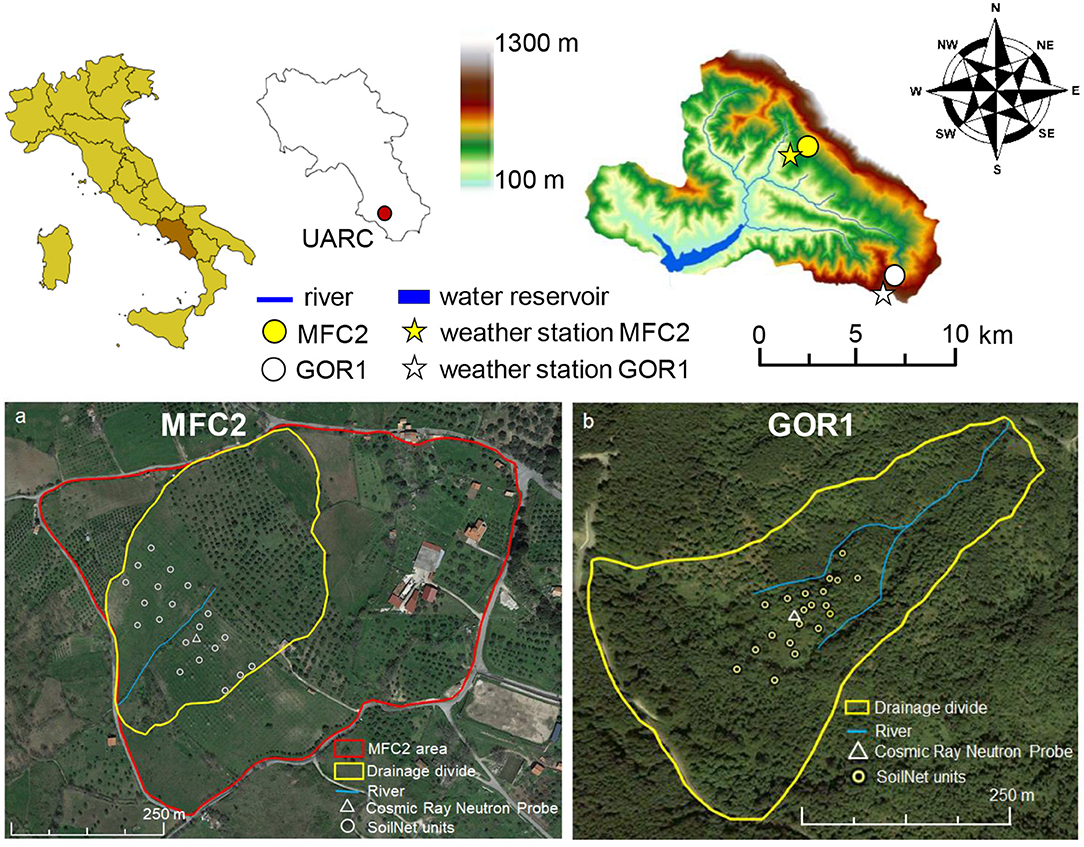
Figure 1. Geographical location and 5-m Digital Elevation Model (DEM) of the Upper Alento River Catchment (UARC) in Campania (southern Italy), with the two experimental sites (MFC2 and GOR1) and corresponding weather stations displayed in the upper plots. The artificial water reservoir is delimited by the Piano della Rocca earthen dam. The layouts of the 20 end-devices of the SoilNet wireless sensor network and Cosmic Ray Neutron Probe are displayed on the satellite image (on the bottom plots) at MFC2 (plot a) GOR1 (plot b).

In 2016 and at each of the above-mentioned experimental sites, a SoilNet wireless sensor network (Forschungszentrum Jülich, Germany) was installed comprising twenty end-devices connected to sensors positioned at the soil depths of 0.15 and 0.30 m. At each soil depth, the apparent soil dielectric permittivity (which is used to estimate θ through an empirical calibration relation), soil temperature, and soil electrical conductivity are measured by the GS3 capacitance sensors (METER Group, Inc., Pullman, WA, USA), whereas the soil matric pressure potential, ψ, is determined by the MPS-6 sensor (METER Group, Inc., Pullman, WA, USA). Note that the MPS-6 sensor can measure ψ values only in the range from −90 hPa (i.e., a matric suction head of about 0.92 × 10⁰ m of H₂O) to −10⁶ hPa (i.e., a matric suction head of about 1.02 × 10⁴ m of H₂O) and is, therefore, unable to provide measurements when the soils are near saturation. The SoilNet data are transmitted wirelessly to a local gateway and then via Global System for Mobile Communications (GSM) modem to a central data server in near-real time (Bogena et al., 2010). The SoilNet end-devices were installed around a stationary cosmic-ray neutron probe (CRS2000/B by Hydroinnova LLC, Albuquerque, USA) by covering the experimental sub-catchments as much as possible for future application and validation of hydrological models (Figures 1a,b). The CRNP is a particle detector that measures the neutron intensity in the well-mixed neutron pool above the land surface, which is mainly determined by the amount of hydrogen atoms in the soil. The resulting inverse relationship between soil moisture and neutron intensity is described by the equation proposed by Desilets et al. (2010), where an empirical parameter requires site-specific calibration. The soil volume probed by the CRNP (i.e., in terms of radial footprint and penetration depth) is still a matter of debate, as new theories, additional data, and further interpretations are constantly being added (Köhli et al., 2015). According to Schrön et al. (2017), the CRNP provides indirect measurements of soil moisture over a circular footprint with an effective radius ranging from ~150 to 210 m (i.e., from about 7 to 14 hectares) depending on various factors, e.g., soil moisture, atmospheric pressure, air humidity, vegetation biomass, etc. The CRNP is hyper-sensitive to soil moisture within the immediate vicinity and the sensitivity to soil moisture decreases non-linearly with radial distance (Schrön et al., 2017). The CRNP is most sensitive to soil moisture in the upper soil horizon, and this sensitivity decreases exponentially to a penetration depth of about 0.3–0.8 m depending on the soil moisture content. Therefore, we used the weighting procedure proposed from Schrön et al. (2017) to calculate appropriate mean values of our point-scale soil moisture measurements with the GS3 capacitance sensors installed at soil depths of 0.15 m and 0.30 m for comparisons with our CRNP-based soil moisture measurements.

One automatic weather station is located near MFC2, at 400 m a.s.l., and another near GOR1, at 711 m a.s.l. (Figure 1). Both weather stations are equipped with the same types of sensors for measuring the following variables at hourly time-steps: rainfall (R), air temperature, air relative humidity, wind speed, and direction, and net solar radiation using four-component net radiation sensors (NR01 net radiometer, Hukseflux Thermal Sensors, The Netherlands). According to World Meteorological Organization (WMO) standards, wind speed and air temperature are measured at a height of 3.0 m, whereas solar radiation is measured with the sensors positioned at a height of 2.0 m above the soil surface. Reference evapotranspiration (ET₀) was calculated by using the Penman-Monteith equation according to the protocol proposed by Allen et al. (1998).

At each position of the SoilNet end-devices, disturbed soil samples were collected at the two sensing depths for the laboratory determination of the soil particle-size distribution (PSD). Undisturbed soil cores (steel cylinder of 0.072 m inner diameter and 0.070 m height) were also collected at the soil depth of 0.15 m (vertical sampling at a soil depth of 0.115–0.185 m) of each measuring position to determine oven-dry soil bulk density (ρ_b).

Table 1 lists the descriptive statistics of United States Department of Agriculture (USDA) soil particle classes (sand, silt, and clay contents expressed in percentages) at the two soil depths (0.15 and 0.30 m) as well as the oven-dry soil bulk density and soil porosity at a soil depth of 0.15 m for the 20 SoilNet units in both MFC2 and GOR1 (see also Tables A1, A2 in the Appendix reporting measurements of soil physical properties at each location). The individual triplet of sand-silt-clay percent is inserted in the USDA soil textural triangle of Figure 2, showing that the MFC2 cropland site is dominated by the clay and silty-clay-loam textural classes, whereas the predominant soil textural class of the GOR1 woodland site is loamy.

TABLE 1

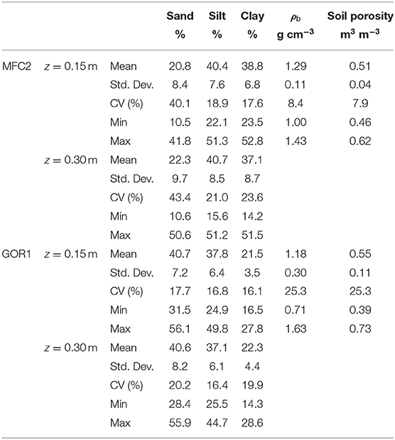
Table 1. Descriptive statistics of sand, silt, and clay contents (in percent) at the two sampled soil depths (0.15 and 0.30 m) and oven-dry soil bulk density (ρ_b) with corresponding soil porosity at the soil depth of 0.15 m in the 20 SoilNet units for both MFC2 and GOR1 sub-catchments.

FIGURE 2

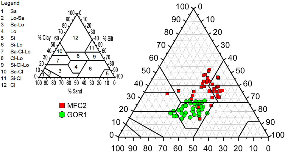
Figure 2. USDA soil textural classes (Sa = sand; Lo = loam; Si = silt; Cl = clay) of the 20 soil samples collected at each of the two soil depths (0.15 and 0.30 m) at MFC2 (red squares) and GOR1 (green circles).

At MFC2 and GOR1, the mean and standard deviation values of the textural particles are virtually the same for both sensing soil depths. Therefore, the shallow soil layer of both sites can be considered quite uniform in terms of soil properties. However, the mean sand content at MFC2 is almost half that at GOR1, thus offering a first glimpse of the diversity between the two experimental sites. Mean oven-dry soil bulk density (ρ_b) values measured at the soil depth of 0.15 m are also virtually the same at both MFC2 and GOR1, but the spatial variability of ρ_b is slightly higher in the forested site. Mean soil porosity is computed from the knowledge of ρ_b, assuming the soil particle density always equal to 2.65 g cm⁻³.

Table 2 reports the descriptive statistics of the following terrain attributes: elevation (ζ), slope tangent, surface curvature (κ), aspect (in degrees), and upslope contributing area (A_c). The elevation of the forest site is almost twice that of the agricultural site. The high steepness at GOR1 induces a wide range of elevation (almost 100 m) of the SoilNet end-device positions, whilst MFC2 has gentle slopes and hence a very narrow elevation range (about 20 m). The two sites have similar curvature, but different slope aspect as described above.

TABLE 2

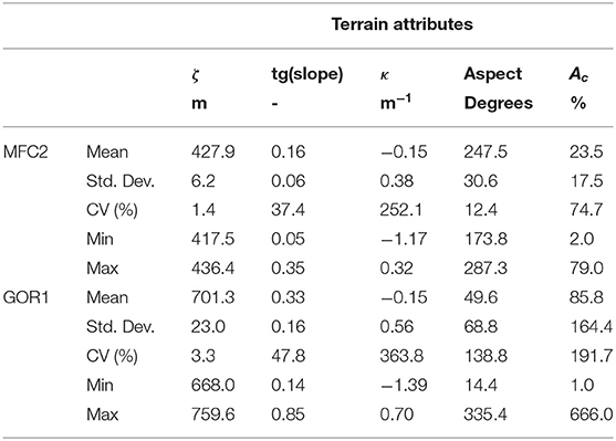
Table 2. Descriptive statistics of terrain attributes, namely elevation (ζ, above mean sea level), tangent of slope [tg(slope)], tangential curvature (κ), aspect, and upslope contributing area (A_c) for the 20 SoilNet units in both MFC2 and GOR1 sub-catchments.

Calibration Procedure for Invasive and Non-invasive Soil Moisture Sensors

A calibration step is necessary for ensuring good accuracy and precision when estimating point-scale and field-scale soil moisture values from the soil dielectric properties measured by capacitance sensors (Bogena et al., 2017; Gasch et al., 2017; Domínguez-Niño et al., 2019) and from neutron counts measured by CRNP (Franz et al., 2013; Baroni et al., 2018), respectively. Calibration of the CRNP requires simultaneous measurements of soil moisture using the thermogravimetric method and neutron intensity measured by the CRNP to estimate the area-wide soil moisture, θ_CRNP. We followed the calibration protocol suggested by Heidbüchel et al. (2016) and conducted three field campaigns to cover both wet and dry climate conditions to account for local climate seasonality. Soil sampling was carried out using a stainless steel core sampler with a plastic liner inside, with a length of 0.30 m and an inner diameter of 0.05 m. The soil samples were collected in 18 positions around the CRNP (six locations along radial distances of 1.0, 10.0, and 110.0 m). Each plastic liner was then cut into six pieces (each of 0.05 m length) to measure the oven-dry soil bulk density and soil-water content with the thermogravimetric method. Therefore, for each experimental sub-catchment, a total of 108 undisturbed soil cores were collected in each field campaign. The annex to this paper provides the Excel file employed for the calculations of the calibration procedure (Heidbüchel et al., 2016).

For calibrating the GS3 capacitance sensors, we carried out five field campaigns to collect undisturbed soil cores with the same core sampler used for calibrating the CRNP. The soil samples were collected over the twenty positions of the SoilNet end-devices. After soil sampling, we cut each core into six sub-cores (each of 0.05 m in length) to measure the soil moisture value by the thermogravimetric method and also the particle-size distribution. For calibration purposes, only the two sub-cores relating to the soil depths of 0.15 and 0.30 m were considered. To convert the apparent soil dielectric permittivity, ε_a, into the GS3-based soil moisture, θ_GS3, we used the relation proposed by the METER company (Ferrarezi et al., 2020):

$\begin{array}{l}{\theta }_{GS3}=5.89·10^{-6}{\epsilon }_a^3-7.62·10^{-4}{\epsilon }_a^2+3.67·10^{-2}{\epsilon }_a\\ -7.53·10^{-2},& (1)\end{array}$

which was validated with the soil moisture values determined in our laboratory with the thermogravimetric method (not shown in this paper).

Two MPS-6 sensors were tested and calibrated in the laboratory using a pressure plate apparatus in a way similar to that described by Malazian et al. (2011). Finally, the empirical equation was used to compensate for the temperature effect on soil matric potential measured by the MPS-6 sensor (see Equation (3) in Walthert and Schleppi, 2018).

For both sub-catchments, the monitoring program started in spring 2016. Daily (indicated by the subscript d) values of rainfall, R_d, and reference evapotranspiration, ET_0,d, together with the soil moisture content time series are shown in Figure 3 for MFC2 and in Figure 4 for GOR1.

FIGURE 3

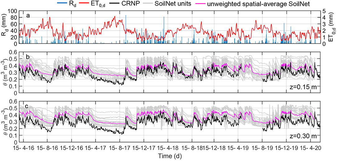
Figure 3. Daily values of (a) rainfall, R_d (blue bars), reference evapotranspiration, ET_0,d (red line), (b) SoilNet-based soil moisture contents (gray lines) at 0.15 m soil depth at the 20 locations and their unweighted spatial-mean (magenta line) and CRNP-based soil moisture (black line) and (c) SoilNet-based soil moisture contents (gray lines) at 0.30 m soil depth at the 20 locations and their unweighted spatial-mean (magenta line) and CRNP-based soil moisture (black line) at MFC2.

FIGURE 4

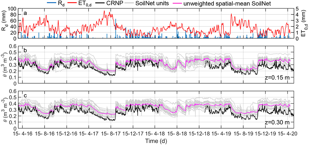
Figure 4. Daily values of (a) rainfall, R_d (blue bars), reference potential evapotranspiration, ET_0,d (red line), (b) SoilNet-based soil moisture contents (gray lines) at 0.15 m soil depth at the 20 locations and their unweighted spatial-mean (blue line) and CRNP-based soil moisture (black line) and (c) SoilNet-based soil moisture contents (gray lines) at 0.30 m soil depth at the 20 locations and their unweighted spatial-mean (blue line) and CRNP-based soil moisture (black line) at GOR1 site.

The presence of sporadic sensor malfunctioning of the GS3 sensors appears in these graphs due to the abrupt voltage drops of some batteries. Unfortunately, the CRNP at GOR1 (from June 2018 to January 2019) and at MFC2 (from April 2019 to July 2019) experienced a fault because of the modem interruption. The CRNP measurements, θ_CRNP, were affected by episodic spikes during the rainy season probably because of water ponding, low air temperature on the soil surface, or water being retained by leaf interception. Therefore, such values were removed from the data analysis.

Table 3 reports the descriptive statistics of SoilNet-based (θ_GS3) and CRNP-based (θ_CRNP) soil moisture, rainfall (R_a), cumulative reference potential evapotranspiration (ET_0,a) depths on an annual (indicated by subscript a) basis over the years 2017, 2018, and 2019. It is worth noting that the year 2017 was characterized by a notable meteorological drought, with R_a being about <41.5% in 2018 and <33.2% in 2019 for the cropland area and <31.4% in 2018 and <8.5% in 2019 for the forested area. During these 3 years, the mean annual rainfall in GOR1 was constantly and noticeably less than in MFC2, whereas the mean annual potential evapotranspiration ET_0,a in GOR1 was only slightly less than in MFC2.

TABLE 3

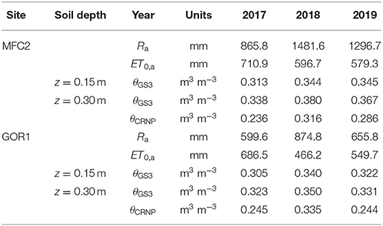
Table 3. Rainfall (R_a) and reference potential evapotranspiration (ET_0,a) depths on an annual basis with corresponding spatio-temporal-mean of SoilNet-based soil moisture (θ_GS3) at soil depths of 0.15 and 0.30 m and time-averaged CRNP-based soil moisture (θ_CRNP) at MFC2 and GOR1 in 2017, 2018, and 2019.

Data Analysis for Assessing Temporal Variability of the Soil Moisture Index

The soil moisture index (SMI_j) at time j provides a rough quantification of soil wetness and was computed in this study according to Hunt et al. (2009):

$\begin{array}{ll}SM{I}_j=-5+10\frac{({\theta }_j-{\theta }_{WP})}{({\theta }_{FC}-{\theta }_{WP})}& (2)\end{array}$

where θ_j is soil moisture content at time j, θ_FC is soil moisture at the condition of “field capacity” in the soil profile, and θ_WP is soil moisture when on average a plant wilts permanently, being unable to recover its turgor. Note that the difference θ_FC-θ_WP is commonly defined as the Plant Available Soil Water Holding Capacity (Romano and Santini, 2002). SMI takes on negative and positive values indicating the presence of soil conditions from relatively dry to driest (−5 ≤ SMI <0) or from relatively wet to wettest (0 ≤ SMI ≤ +5). The values SMI = −5 correspond to the soil moisture content at “permanent wilting,” whereas SMI = +5 is indicative of the soil moisture content at “field capacity” (Hunt et al., 2009).

The permanent wilting point (θ_WP) is commonly computed from the knowledge of the soil WRF, θ(ψ), as θ at the matric pressure potential ψ = −15,300 hPa [i.e., 15 bars; Romano and Santini (2002)], and this criterion is employed in the present study. Instead, the condition of “field capacity” in a soil profile does not have a clear and shared definition and is still subjected to slightly different meanings. Actually, the soil moisture content at “field capacity,” θ_FC, is a process-dependent parameter that can be defined as the average soil moisture measured in the entire soil profile when the water flux at its lower boundary becomes virtually nil during a drainage process starting with the initial condition of full saturation and with evaporation prevented at the upper boundary of soil surface (Romano and Santini, 2002; Nasta and Romano, 2016). This parameter is considered a critical threshold of soil water-holding capacity and commonly employed in bucketing-type models to control hydrological processes, such as overland flow and drainage below the root zone of a uniform soil profile (Romano et al., 2011). The value of θ_FC should be obtained using a specifically designed in-situ drainage experiment, but can be conveniently retrieved also through numerical simulations, especially in the case of layered soil profiles that are the rule rather than an exception in the real world (Nasta and Romano, 2016). Under simplified assumptions and in the case of a uniform soil profile, the value of θ_FC can instead be roughly estimated from the knowledge of the soil WRF using a static criterion that assumes, on average, that θ_FC is equal to the soil-water content at the matric pressure potential of −330 hPa. Allowing for the effect of soil texture on the “field capacity” value, Romano and Santini (2002) suggested setting a soil matric pressure potential of ~-100 hPa for coarse soils and −500 hPa for fine soils. The matric pressure value of −330 hPa should be mostly used in the cases of medium-textured soils (Romano et al., 2011).

Given the simplified picture of soil condition offered by the SMI, in this study we estimated the θ_FC value through the analytical equation proposed by Assouline and Or (2014) that computes the soil matric potential at “field capacity” (ψ_FC) as follows:

$\begin{array}{ll}{\psi }_{FC}=\frac{1}{{\alpha }_{vG}}{\left(\frac{n_{vG}-1}{n_{vG}}\right)}^{(\frac{1-2n_{vG}}{n_{vG}})},& (3)\end{array}$

and hence determines the soil moisture content at field capacity as follows:

$\begin{array}{ll}{\theta }_{FC}={\theta }_r+({\theta }_s-{\theta }_r){\left[1+{({\alpha }_{vG}|{\psi }_{FC}|)}^{n_{vG}}\right]}^{\left(\frac{1-n_{vG}}{n_{vG}}\right)},& (4)\end{array}$

where α_vG (hPa⁻¹) and n_vG (–) are the two shape parameters featuring in van Genuchten (1980) analytical soil-water retention relationship θ(ψ):

$\begin{array}{ll}\theta (\psi )={\theta }_r+\frac{{\theta }_s-{\theta }_r}{{(1+|{\alpha }_{vG}\psi {|}^{n_{vG}})}^{m_{vG}}},& (5)\end{array}$

with the condition m_vG = 1–1/n_vG. We use the acronym “vG” as a subscript to refer to the above parameters. The θ_s (m³ m⁻³) and θ_r (m³ m⁻³) parameters are the saturated and residual soil water contents, respectively. While θ_s has a clear physical meaning and is measured with laboratory or field tests, θ_r is often set at zero or assumed as an additional unknown parameter to be estimated by the fitting procedure together with the other two unknown parameters α_vG and n_vG. By substituting Equation (3) into Equation (4), the knowledge of θ_s, θ_r, and n_vG, allows to determine θ_FC through the following closed-form expression:

$\begin{array}{ll}{\theta }_{FC}={\theta }_r+({\theta }_s-{\theta }_r){\left\{1+{\left[\frac{n_{vG}-1}{n_{vG}}\right]}^{(1-2n_{vG})}\right\}}^{\left(\frac{1-n_{vG}}{n_{vG}}\right)}.& (6)\end{array}$

To test whether the SMI distributions are unimodal or bimodal, in this study we refer to the empirical method that evaluates a bimodality coefficient, termed BC (Pfister et al., 2013), which ranges between 0 and 1 and is computed as follows:

$\begin{array}{ll}BC=\frac{m_3^2+1}{m_4+3\left[{(n-1)}^2/(n-2)(n-3)\right]},& (7)\end{array}$

where n is the sample size, m₃ is the skewness and m₄ is kurtosis of the distribution. To avoid sample bias, the skewness and kurtosis values are calculated as follows:

$\begin{array}{ll}{m}_3=\frac{\sqrt{n(n-1)}}{n-2}\left\{\frac{1/n{\displaystyle {\sum }_{i=1}^n}{(x_i-\overline{x})}^3}{{\left[\sqrt{1/n{\displaystyle {\sum }_{i=1}^n}{(x_i-\overline{x})}^2}\right]}^3}\right\},& (8)\end{array}$

$\begin{array}{l}{m}_4=\frac{n-1}{\left(n-2\right)\left(n-3\right)}\{\left(n+1\right)\frac{1/n{\displaystyle {\sum }_{i=1}^n{\left(x_i-\overline{x}\right)}^4}}{{\left[1/n{\displaystyle {\sum }_{i=1}^n{\left(x_i-\overline{x}\right)}^2}\right]}^2}\\ -3\left(n-1\right)\},& (9)\end{array}$

where $\overline{x}$ is the arithmetic mean of the set of data. A bimodal distribution is characterized by high skewness, low kurtosis, or both. Specifically, if BC is >0.555 (BC > 0.555), then the hypothesis that the data follow a bimodal distribution cannot be rejected (Kang and Noh, 2019).

Data Analysis for Assessing Spatial Variability of Soil Moisture Data

The partial least-squares regression (PLSR) model is used to reveal the factor explaining the spatial variance of daily soil moisture data. As discussed in (Romano and Chirico, 2004) and Nasta et al. (2018b), most soil moisture variations are cross-correlated with soil physical properties, such as the percentages of sand, silt, and clay contents (see Table 1 and Tables A1, A2), as well as terrain attributes, such as elevation above mean sea level, slope aspect, slope gradient, tangential curvature, and upslope contributing area (see Table 2). The PLSR model generates new predictor variables (components) as combinations of the original predictors and finds combinations of the predictors that have a large covariance with the soil moisture data. The predictive ability of PLSR is expressed in terms of the coefficient of determination and root mean squared error (RMSE) which, respectively, evaluate the scatter of the data points around the fitted regression curve and the bias between observed and modeled soil moisture values. PLSR also provides the percent of variance explained by the components, distinguishing between soil textural characteristics and topographic attributes.

Results

Assessing the CRNP Vertical Footprint

In this study, we investigated the vertical footprint of the CRNP in the two experimental areas (MFC2 and GOR1). Among the variety of weighting procedures provided in the literature, we opted to use the equal (unweighted) spatial-mean and a reliable physically-based weighted spatial-mean of point-scale soil moisture measurements (Schrön et al., 2017). The first step is to compare the CRNP-based soil moisture with the unweighted soil moisture spatial-mean, as depicted in Figures 3, 4. We also computed the physically-based weighted spatial-mean of the SoilNet-based soil moisture data as recommended by Schrön et al. (2017) by using the MATLAB script provided by these authors. The comparisons between the CRNP-based soil moisture and all the unweighted or weighted spatial-mean SoilNet-based soil moisture are depicted in the scatter plots of Figure 5 for both the MFC2 and GOR1 sites. Although RMSE takes on very similar values for the four cases considered, the Schrön et al. (2017) weighted procedure seems to provide a slightly better correlation than the unweighted one especially at the higher soil moisture contents, as evident from the fact that the scatter cloud tends to be closer to the identity line as θ increases. This situation is more pronounced for MFC2 than GOR1. It is also worth noting that the scatter cloud increasingly diverges from the identity line when soil moisture values decrease. Overall, the impact of employing a weighting procedure for our case studies seems to provide only a scant improvement. This situation can be explained if one considers that, allowing for the limited number of available devices, the positioning of the sensor nodes was primarily designed to detect the spatial patterns of the soil hydrological variables as well as possible and not for comparison purposes between the two sensing systems (i.e., a relatively low number of SoilNet end-devices is located in the direct vicinity of the CRNP). That said, in the following we assumed that both vertical and radial weights also apply to obtain the averaged soil matric potential values.

FIGURE 5

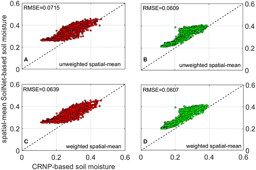
Figure 5. Relation between CRNP-based soil moisture and unweighted spatial-mean of SoilNet-based soil moisture at (A) MFC2; (B) GOR1; relation between CRNP-based soil moisture and weighted spatial-mean of SoilNet-based soil moisture at (C) MFC2; (D) GOR1. Dashed black line depicts the 1:1 identity line. RMSE values are reported in each subplot.

Because the soil moisture values observed by the two sensing systems show different means and ranges of variation, the comparison among the time series is more robust when these data are standardized using the Z-scores, which can take on positive or negative values (for example, positive values indicate that the data are above the arithmetic mean). As evident from a perusal of Figure 6, both unweighted and weighted time series of θ_GS3 overlap almost perfectly over the CRNP-based soil moisture time series. Nevertheless, the CRNP data show significantly higher temporal variability, thus indicating a stronger response to climate forcing. This feature reflects the higher sensitivity of the CRNP to near-surface soil moisture due to the decreasing sensitivity with soil depth (Schrön et al., 2017).

FIGURE 6

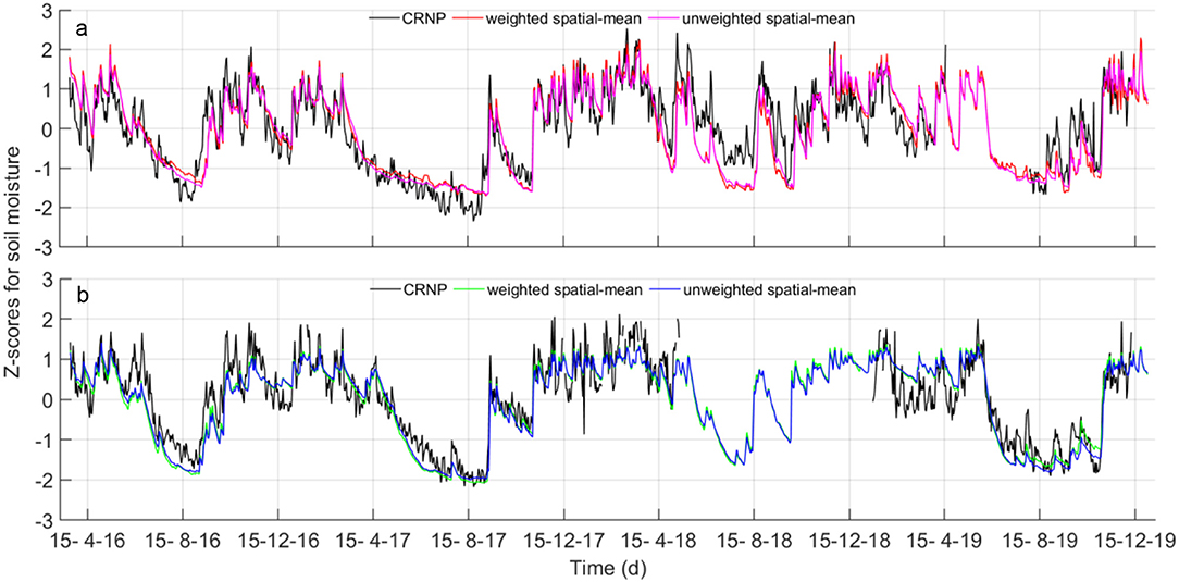
Figure 6. Daily values of Z-scores of unweighted spatial-mean SoilNet-based soil moisture contents, weighted spatial-mean and CRNP-based soil moisture (black line) in (a) MFC2; and (b) GOR1.

Field-Scale Soil Water Retention Characteristics

The simultaneous availability of soil moisture, θ_{GS3, j}, and matric pressure head, ψ_j, values, at the same time, j, and soil depth, z, from the wireless sensor networks, allows us to identify the SoilNet-based soil water retention functions (WRFs) at the two sites. The WRFs of Figures 7A,B, shown for the two sensing depths of 0.15 and 0.30 m, were determined by coupling the daily unweighted values of the spatial-mean of θ_{GS3, j}and log₁₀-transformed ψ_j. Because the MPS-6 sensor is unable to measure matric pressures >-90 hPa, data pairs |ψ_j|-θ_{GS3, j} are not available in the near-saturated region of the WRF. Consequently, we set the saturated soil water content, θ_s, as 90% of the spatial-mean soil porosity obtained from the direct measurements of ρ_b (see Table 1). Figures 7A,B also show van Genuchten's water retention relations whose unknown parameters α_vG and n_vG were obtained by non-linear regression, while setting θ_r at zero. All parameters, including the prescribed (θ_s), optimized (α_vG, n_vG), and those derived from the knowledge of the WRFs (θ_FC, θ_WP) are reported for each site in Table 4 with the corresponding RMSE values. Overall, the two SoilNet-based WRFs belonging to the MFC2 and GOR1 sites (solid black line for GOR1 and dashed black line for MFC2) are characterized by different shapes, with the solid curve of GOR1 showing a shape typical for medium- or coarser-textured soils, with a quite rapid decrease in soil moisture contents in the wet region of the diagram. The dashed curve for MFC2 desaturates with a smooth decay which certainly reflects the typical behavior of finer-textured soils.

FIGURE 7

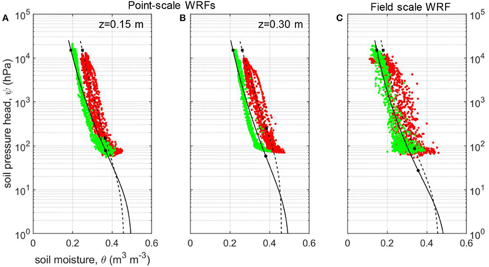
Figure 7. Soil-water retention functions obtained by relating daily values of (A) SoilNet data pairs at z = 0.15 m; (B) SoilNet data pairs at z = 0.30 m; (C) CRNP-based soil moisture (θ_{CRNP, j}) and spatial-mean SoilNet-based soil matric potential (absolute value |ψ_j|) at MFC2 (red circles) and GOR1 (green circles). Dashed black (MFC2) and solid black (GOR1) lines represent the soil-water retention curves fitted using van Genuchten's parametric relation. Black circles and black squares denote the θ_FC and θ_WP values at the conditions of “field capacity” and “permanent wilting,” respectively.

TABLE 4

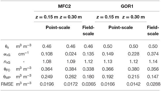
Table 4. Parameters feauturing in the vG-WRF at MFC2 and GOR1 referring to point-scale SoilNet based WRF at soil depths of 0.15 and 0.30 m and field-scale WRF.

According to our method and as depicted in Figure 7C, an “effective” (field-scale) soil WRF over the CRNP footprint can be suitably obtained by coupling, for the same time j, the areal-based soil moisture (θ_{CRNP, j}) contents with the weighted spatial-mean matric pressure potential (ψ_j) values. The weights applied to ψ_j-values were obtained through the weighting procedure recommended by Schrön et al. (2017).

In all the soil water retention curves of Figure 7, the black circles identify the soil moisture contents at “field capacity,” as computed by Equation (6), and the black squares identify the soil moisture contents at “permanent wilting,” corresponding to |ψ| = 1.50 × 10⁴ hPa. The picture provided by the θ_CRNP(|ψ|) retention curves of Figure 7C allows us to frame in a new perspective the potential of using the areal soil moisture contents offered by a CRNP, and also gives us some preliminary indications on possible drawbacks related to a scale mismatch between the areal θ and the point-scale ψ data. For both MFC2 and GOR1 sites, the observed scatter of the retention points (see RMSE values in Table 4) is likely due to the different spatial scales associated with the CRNP-based soil moisture contents and the point-measured matric potential pressure values.

Temporal Variability of the Soil Moisture Index

The soil moisture index (SMI) is a transformation of soil moisture data and was employed in this study to remove (i) the offset between CRNP-based and SoilNet-based soil moisture observed in Figures 3–5, and (ii) the impact of time-invariant environmental controls, such as the soil textural characteristics and topographical features, on the soil moisture temporal variability (Mittelbach and Seneviratne, 2012). The SMI is computed by using the soil moisture contents at “field capacity” (θ_FC) and “permanent wilting” (θ_WP) as determined in section Field-Scale Soil Water Retention Characteristics and reported in Table 4 (see also the plots in Figure 7) following the procedure described in section Data Analysis for Assessing Temporal Variability of the Soil Moisture Index.

Based on the results shown by Romano et al. (2018) regarding the soil moisture distributions, we further processed our datasets by analyzing the histograms of daily SMI values (SMI_d) that are depicted in Figure 8. The individual graphs of this figure enable us to suitably compare the hydrological responses of the cropland (red bars) and woodland (green bars) areas. The SMI_d values mostly fluctuate around the zero value with the occurrence of wetter-than-normal conditions induced by rainfall surplus and drier-than-normal conditions determined by rainfall deficits. Note that the period from March to September 2017 was characterized by an exceptionally long dry spell. For almost all months over the investigated 4-year period, the rainfall at MFC2 exceeded that at GOR1, which is reflected in the amount of water present in the soil.

FIGURE 8

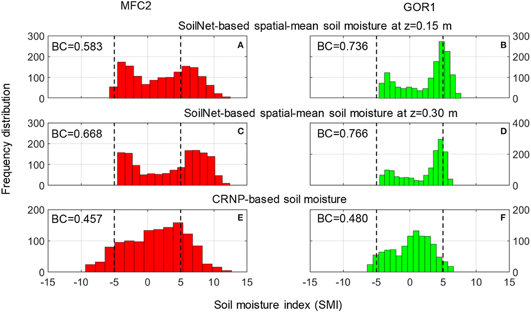
Figure 8. Frequency distributions of daily values of SMI (SMI_d) calculated using SoilNet-based soil moisture spatial-mean at z = 0.15 m at (A) MFC2 and (B) GOR1, and z = 0.30 m at (C) MFC2 and (D) GOR1, and CRNP-based soil moisture at (E) MFC2 and (F) GOR1. Each subplot reports the bimodality coefficient (BC).

The graphs of Figure 8 show that the histograms of SMI_d computed from the θ_GS3 data, at the two soil depths of 0.15 and 0.30 m, are characterized by an evident bimodal shape and this visual evidence is also quantified by the bimodal coefficient BC, which always takes on values >0.555. In contrast, the histograms of SMI_d obtained from the θ_CRNP data follow a more Gaussian-like unimodal distribution, as indicated by BC values lower than 0.555. A perusal of these plots provides a useful indication of the soil hydrological behavior of these two experimental sites. Inspection of Figures 3, 4 highlights that the soil moisture time series measured by the GS3 sensors show the presence of persistent wet and dry conditions that are interrupted by sharp wetting pulses and smooth soil desaturation. The two observed long-term plateaus induce the bimodal shape of the corresponding distribution of SoilNet-based SMI_d values that reflect the typical rainfall seasonality of the Mediterranean climate (Vilasa et al., 2017). By contrast, CRNP-based soil moisture data show a constant decrease during desaturation in the growing season and sharp wetting-drying pulses during the rainy season. This temporal variability is typical of the near-surface soil moisture dynamics and is reflected in the unimodal frequency distribution of CRNP-based SMI_d values in Figure 8. Nevertheless, a further step is to verify whether these patterns hold within a year-by-year analysis given the remarkable variability of annual rainfall sums reported in Table 3. Figures 9, 10 report the frequency distributions of SMI_d values calculated by using SoilNet-based soil moisture at z = 0.15 m and CRNP-based soil moisture for each year at MFC2 and GOR1, respectively. Interestingly, CRNP-based soil moisture is able to capture bimodality only in 2017 (characterized by a long drought) in MFC2 (BC = 0.57). Extremely wet conditions recorded in 2018 induce a unimodal normal distribution in CRNP-based SMI_d values in MFC2. Unfortunately, a similar situation could not be explored in GOR1 due to a large amount of missing data at this site.

FIGURE 9

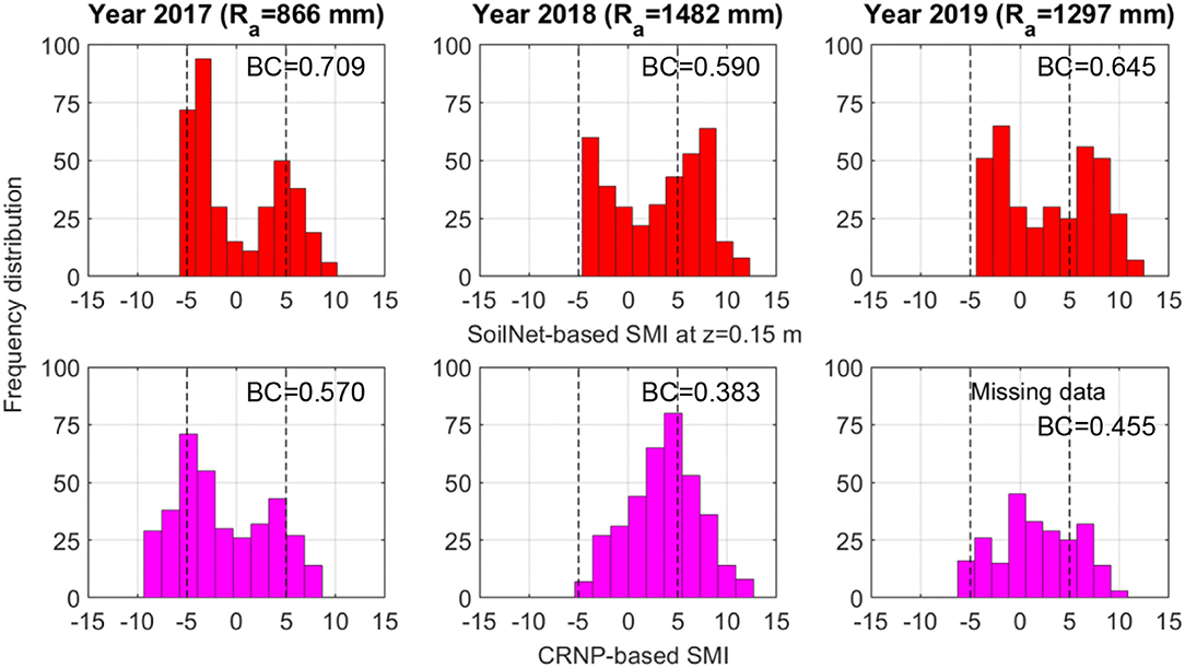
Figure 9. Frequency distributions of daily values of SMI (SMI_d) calculated using SoilNet-based soil moisture at z = 0.15 m (red bars) and CRNP-based soil moisture (magenta bars) at MFC2 in 2017, 2018, and 2019. Each subplot reports the bimodality coefficient (BC).

FIGURE 10

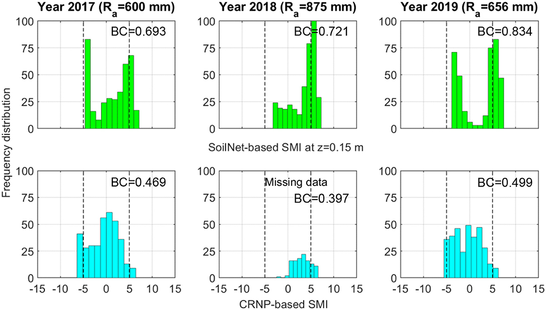
Figure 10. Frequency distributions of daily values of SMI (SMI_d) calculated with SoilNet-based soil moisture at z = 0.15 m (green bars) and CRNP-based soil moisture (cyan bars) at MFC2 in 2017, 2018, and 2019. Each subplot reports the bimodality coefficient (BC).

Spatial Variability of Soil Moisture

This section illustrates the spatial variability of SoilNet-based soil moisture explained by easily-available environmental variables such as soil textural classes and terrain features. Figure 11 illustrates the CRNP-based SMI_d values against the spatial-standard deviation of θ_GS3,j values measured at the soil depth of 0.15 m in both MFC2 and GOR1. The spatial variability of soil moisture data is related to SMI_d values with a somewhat concave downward shape that is more pronounced for the forested site. This shape is similar to that reported by, for example, Teuling and Troch (2005), Famiglietti et al. (2008), and Rosenbaum et al. (2012), although different patterns of this relationship have been reported elsewhere (Mittelbach and Seneviratne, 2012). Because of the larger spatial variability of soil properties in the cropland site, one immediately notices the larger scatter of the points for MFC2 (Figures 11A,B) with respect to GOR1 (Figures 11C,D) in the central range of the catchment's spatially averaged soil moisture measured by the CRNP. This may explain the large scatter observed in the field-scale WRF belonging to MFC2 (Figure 7C). Further insights are gained by evaluating the role exerted by easily-retrievable local and non-local factors, comprising the five topographical attributes (elevation, aspect, slope, tangential curvature, upslope contributing area) and the three soil textural classes (percentages of sand, silt, and clay content), to help describe the spatial organization of the observed soil moisture datasets. However, apart from a few general comments, we caution the reader that the impact of vegetation was neglected in this study due to a lack of direct robust measurements.

FIGURE 11

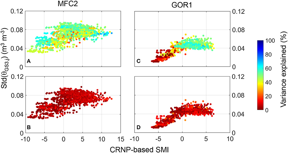
Figure 11. Scatter plots of CRNP-based SMI-values against spatial standard-deviation of SoilNet-based soil moisture, Std(θ_GS3,j), at 0.15 m soil depth and time j for the two experimental sites. The various shades of the colored circles indicate the amount (in percent) of spatial variance explained: (A) by terrain attributes at MFC2; (B) by soil texture at MFC2; (C) by terrain attributes at GOR1; (D) by soil texture at GOR1.

The variability explained by the soil terrain attributes (top panels, Figure 11A for MFC2 and Figure 11C for GOR1) and textural characteristics (bottom panels, Figure 11B for MFC2 and Figure 11D for GOR1) is quantified by using the PLSR method (described in section Data Analysis for Assessing Spatial Variability of Soil Moisture Data) and represented by the color bar on the right side of the plots in Figure 11. It is worth noting that, on average, the terrain attributes explain almost 50% of soil moisture spatial variability in the case of the cropland site (i.e., MFC2), under both wet and dry conditions. In the forested site (i.e., GOR1), the considered terrain attributes explain on average about 40% of soil moisture spatial variability. Nonetheless, this percentage of explained variability increases significantly under wet conditions (bluish colors in Figure 11C) and decreases considerably under dry conditions (reddish colors in Figure 11C). Figures 11B,D show that soil texture has a scant ability to explain the spatial organization of soil moisture data in both sites at the soil depth of 0.15 m.

The five terrain attributes (elevation, aspect, slope, tangential curvature, upslope contributing area) explain most near-surface soil moisture variability in both sites. Interesting aspects emerge if we iteratively repeat the PLSR exercise by removing one terrain attribute at a time: aspect-induced variability of soil moisture plays a major role in both experimental sites; the second-ranked topographic attribute is elevation for MFC2, and upslope contributing area for GOR1.

Discussion

Drawbacks in Setting Up the Field-Scale Water Retention Function

In this study, we proposed to construct an “effective” (field-scale) soil WRF by coupling the areal-based soil moisture (θ_CRNP,j) contents with the weighted spatial-mean matric pressure potential (ψ_j) values with weights obtained through the weighting procedure recommended by Schrön et al. (2017). On the one hand, a persistent offset occurs between the spatial-mean θ_GS3 and θ_CRNP (see Figures 3, 4) mostly to be attributed to calibration effects; on the other, we observed a relatively large scatter among the water retention data pairs of Figure 7 which may be attributed to several drawbacks. Enhancing the calibration procedure for the CRNPs is certainly to be considered a priority and more field campaigns would probably be required under extremely dry or wet conditions. However, the onset of a sort of scale mismatch represents another important issue which, however, can be tempered by installing some MPS-6 sensors at depths much closer to the soil surface and over more locations, especially near the CRNP (within a radial distance of 5 m). The biomass of dense understory vegetation during the summer season may have influenced the neutron counts determined by the CRNP (Baatz et al., 2015; Jakobi et al., 2018), and the corresponding impact on soil moisture estimates needs more attention in the near future.

To some extent, we used the SMI values to remove the effect of sensor calibration on both the offset and impact of environmental conditions between the two experimental sites. An analysis of the time series of SMI_d values highlights the different behavior between the CRNP-based and SoilNet-based soil moisture contents. The SMI from the sensor networks at soil depths of 0.15 and 0.30 m was able to reflect the impact of Mediterranean rainfall seasonality (Nasta et al., 2020b), although the possibility of having additional capacitance sensors installed at a shallower soil depth would have helped us to better compare our two sensing systems (Franz et al., 2012).

Shortcomings Related to the Calculation of the Soil Moisture Index

In this study, we assumed that the soil moisture index (SMI) can give a useful picture of the soil hydrological behavior of zones with quite different physiographic characteristics, such as our MFC2 and GOR1 experimental sites. Yet the calculation of SMI values requires knowledge of soil moisture contents at field capacity and permanent wilting which, in turn, should be at least retrieved from the soil WRF. If an analytical θ(ψ) relation cannot be obtained from direct measurements, one can resort to a pedotransfer function (PTF) (van Looy et al., 2017) and then compute the values of θ_FC and θ_WP for example by following the static approaches proposed by Assouline and Or (2014) or Reynolds (2018). Alternatively, Guber et al. (2006) reported a list of PTFs to directly estimate the soil moisture contents at the prescribed matric suction pressure |ψ| of 330 hPa (field capacity) and 15,300 hPa (wilting point).

Another question concerns the lack of direct measurement of the soil moisture content at full saturation, θ_s. We assumed θ_s as 90% of the spatial-mean soil porosity, which was calculated from the spatial-mean soil bulk density as suggested by Pollacco et al. (2013). To better support non-invasive measurement methods, such as cosmic-ray neutron sensing, we will shortly carry out field campaigns to measure θ_s at both experimental sub-catchments.

The observed area-wide θ_CRNP values are on average lower than θ_GS3 values (see Table 3). The sensitivity of the CRNP exponentially decreases with depth, with most information on θ_CRNP being concentrated in the first 0.05 m of soil depth, which is not covered by the SoilNet sensors. The differences between SoilNet-based and CRNP-based soil moisture data can definitely affect the determination of the WRF, hence yielding different θ_FC and θ_WP values and consequently different SMI-values (Table 4). In MFC2 the SoilNet-based WRFs lead to field capacity and wilting point values other than those obtained by the CRNP-based WRF (θ_FC = 0.338 m³ m⁻³ and θ_WP = 0.180 m³ m⁻³). Similarly, at GOR1 the SoilNet-based WRFs lead to field capacity and wilting point values different from those obtained by the CRNP-based WRF (θ_FC = 0.356 m³ m⁻³ and θ_WP = 0.147 m³ m⁻³).

SMI was computed over a period of time (from 2016 to 2019) which may be considered as short for drawing sound conclusions. Therefore, this paper presented only some preliminary results of an ongoing long-term monitoring program underway in the Upper Alento River Catchment. As more data become available, a subsequent paper will explore the relationships between long-term time-series of SMI and climate-based standardized indices, such as the Standardized Precipitation Index (SPI) or Standardized Precipitation-Evapotranspiration Index (SPEI), obtaining robust correlations between meteorological and agricultural/hydrological droughts (Mozny et al., 2012; Martínez-Fernández et al., 2015; Barker et al., 2016). Capturing such relationships is of paramount importance in the decision-making process applied to the management of water resources.

Explaining the Spatial Variability of Soil Moisture Data

Assessing the spatial variability of soil moisture, even over relatively small areas, is challenging and commonly obtained using a large number of sensors sparsely deployed in the uppermost soil layer of a study area and along the soil profiles. This task is prohibitively expensive and laborious, and therefore motivated the present investigation, i.e., to explore whether, and to what extent, non-invasive soil moisture datasets obtained from stationary CRNPs can be assumed as representative of areal values whose spatial variations can be explained, in turn, by easily retrievable controlling factors, such as the soil textural classes and terrain attributes. The practical implication of this outcome concerns, for example, either physically-based or statistically-based downscaling methods enabling high-resolution spatial maps of near-surface soil moisture (at meter grid-size) to be estimated from the cosmic-ray areal measurements (i.e., at hectometer grid-size) (Qu et al., 2015; Nasta et al., 2018a).

An increase in spatial variability of soil moisture as its spatial-mean increases was reported in several studies (Martínez-Fernández and Ceballos, 2003; Molina et al., 2014), but increasing spatial variability with decreasing spatial-mean soil moisture was observed by others (e.g., Famiglietti et al., 2008). Most of the investigations reported in the literature have detected a concave downward shape for the relationship that links the spatial soil moisture variability and the spatial-mean soil moisture (e.g., Rosenbaum et al., 2012; Fatichi et al., 2015) as we also found at GOR1 for the soil depth of 0.15 m.

By exploiting the results from the PLSR method, Figure 11 shows the spatial variance of soil moisture explained by terrain attributes and soil texture. In MFC2, almost 50% of the observed spatial variance of topsoil soil moisture (i.e., that measured at the soil depth of 0.15 m) is explained by non-local controls (terrain attributes); soil texture is instead able to explain only 5% of the total variance.

In the forested site (GOR1), the spatial variance of soil moisture data explained by easily-available soil and terrain factors increases when moving from dry to wet conditions. The maximum amount explained reaches 92% in the wet season. Beaudette et al. (2013) reported that terrain attributes were able to consistently account for 30–70% of the total variance of soil moisture at 0.10 m soil depth, and 10–40% at the soil depths of 0.30 and 0.50 m. Wilson et al. (2004) were able to explain a small component (<30%) of the soil moisture spatial variability in six experimental sites using terrain attributes.

Concluding Remarks

This study explores the feasibility of assessing the soil hydrological behavior of two experimental fields by integrating the area-average soil moisture monitored by CRNP and the spatial-mean of the point-scale soil moisture and soil matric potential values measured by a network of multiple low-cost sensors (SoilNet). An in-depth understanding of the hydrological behavior of a field helps improve the application of suitable hydrological models to run numerical simulations. Nonetheless, the measurement of field-scale near-surface soil moisture is sometimes not sufficient to calibrate and validate hydrological models which, in turn, require the knowledge of the soil water retention function. In the present study, we have proposed a technique for obtaining a field-scale soil water retention function as an alternative to laboratory-based methods that are time-consuming, expensive, and rather unfeasible for large-scale applications. However, some drawbacks need to be considered and better understood at least before a proximal sensor for monitoring soil matric potential comes out in the future. The scale mismatch affecting the scatter in the field-scale WRF can be reduced only at the cost of installing a large number of MPS-6 sensors, especially in the near-surface positions. Yet this would increase costs and might become unpractical. Improving calibration procedures can help reduce the offset between CRNP-based soil moisture and weighted spatial-mean SoilNet-based soil moisture as demonstrated by the strong agreement of their Z-scores. The CRNP is not able to capture the bimodal distribution reflected by the SoilNet-based soil moisture data, except in a very dry year like 2017. Last but not least, the large scatter observed in the field-scale WRF in MFC2 can also be induced by the large spatial variability of soil moisture which, in turn, is largely explained by terrain attributes. If the CRNP-based soil moisture is assumed to be representative of areal values, the practical implication of this outcome opens room for using topography-based downscaling methods enabling high-resolution spatial maps of near-surface soil moisture.

Data Availability Statement

The datasets generated for this study are available on request to the corresponding author.

Author Contributions

NR and PN made the conception and design of this study. All the authors participate in the analysis and interpretation of data.

Funding

The TERENO infrastructure was funded by the Helmholtz Association and the Federal Ministry of Education and Research of Germany. Maintenance activities, data collection, and other equipment are resourced by the University of Naples Federico II and partly supported by MiUR-PRIN Project WATer mixing in the critical ZONe: observations and predictions under environmental changes—WATZON (grant 2017SL7ABC) and the iAQUEDUCT project funded within the Water JPI 2018 Joint Call on Closing the Water Cycle Gap–Sustainable Management of Water Resources.

Conflict of Interest

The authors declare that the research was conducted in the absence of any commercial or financial relationships that could be construed as a potential conflict of interest.

Acknowledgments

We are grateful to the landowners of MFC2 and GOR1 for having allowed the installation of the sensor networks.

Supplementary Material

The Supplementary Material for this article can be found online at: https://www.frontiersin.org/articles/10.3389/frwa.2020.00026/full#supplementary-material

References

Allen, R. G., Pereira, L. S., Raes, D., and Smith, M. (1998). Crop Evapotranspiration: Guidelines for Computing Crop Water Requirements. Rome: Food and Agriculture Organization of the United Nations.

Google Scholar

Assouline S. Or D. (2014). The concept of field capacity revisited: defining intrinsic static and dynamic criteria for soil internal drainage dynamics. Water Resour. Res. 50, 4787–4802. doi: 10.1002/2014WR015475

CrossRef Full Text | Google Scholar

Baatz, R., Bogena, H. R., Hendricks Franssen, H.-J., Huisman, J. A., Montzka, C., and Vereecken, H. (2015). An empirical vegetation correction for soil water content quantification using cosmic ray probes. Water Resour. Res. 51, 2030–2046. doi: 10.1002/2014WR016443

CrossRef Full Text | Google Scholar

Babaeian, E., Sadeghi, M., Jones, S. B., Montzka, C., Vereecken, H., and Tuller, M. (2019). Ground, proximal, and satellite remote sensing of soil moisture. Rev. Geophys. 57, 530–616. doi: 10.1029/2018RG000618

CrossRef Full Text | Google Scholar

Barker, L. J., Hannaford, J., Chiverton, A., and Svensson, C. (2016). From meteorological to hydrological drought using standardised indicators. Hydrol. Earth Syst. Sci. 20, 2483–2505. doi: 10.5194/hess-20-2483-2016

CrossRef Full Text | Google Scholar

Baroni, G., Scheiffele, L. M., Schrön, M., Ingwersen, J., and Oswald, S. E. (2018). Uncertainty, sensitivity and improvements in soil moisture estimation with cosmic-ray neutron sensing. J. Hydrol. 564, 873–887. doi: 10.1016/j.jhydrol.2018.07.053

CrossRef Full Text | Google Scholar

Beaudette, D. E., Dahlgren, R. A., and O'Geen, A. T. (2013). Terrain-shape indeces for modeling soil moisture dynamics. Soil Sci. Soc. Am. J. 77, 1696–1710. doi: 10.2136/sssaj2013.02.0048

CrossRef Full Text | Google Scholar

Bogena, H. R., Herbst, M., Huisman, J. A., Rosenbaum, U., Weuthen, A., and Vereecken, H. (2010). Potential of wireless sensor networks for measuring soil water content variability. Vadose Zone J. 9, 1002–1013. doi: 10.2136/vzj2009.0173

CrossRef Full Text | Google Scholar

Bogena, H. R., Huisman, J. A., Schilling, B., Weuthen, A., and Vereecken, H. (2017). Effective calibration of low-cost soil water content sensors. Sensors 17:208. doi: 10.3390/s17010208

PubMed Abstract | CrossRef Full Text | Google Scholar

Bogena, H. R., Kunkel, R., Krüger, E., Zacharias, S., Pütz, T., Schwank, M., et al. (2012). TERENO–long-term monitoring network for terrestrial research. Hydrol. Wasserbewirtsch. 56, 138–143.

Google Scholar

Brocca, L., Ciabatta, L., Massari, C., Camici, S., and Tarpanelli, A. (2017). Soil moisture for hydrological applications: open questions and new opportunities. Water 9:140. doi: 10.3390/w9020140

CrossRef Full Text | Google Scholar

Desilets, D., Zreda, M., and Ferré, T. (2010). Nature's neutron probe: land surface hydrology at an elusive scale with cosmic rays. Water Resour. Res. 46:W11505. doi: 10.1029/2009WR008726

CrossRef Full Text | Google Scholar

Domínguez-Niño, J. M., Bogena, H. R., Huisman, J. A., Schilling, B., and Casadesús, J. (2019). On the accuracy of factory-calibrated low-cost soil water content sensors. Sensors 19:3101. doi: 10.3390/s19143101

PubMed Abstract | CrossRef Full Text | Google Scholar

Entin, J. K., Robock, A., Vinnikov, K. Y., Hollinger, S. E., Liu, S., and Namkhai, A. (2000). Temporal and spatial scales of observed soil moisture variations in the extratropics. J. Geophys. Res. 105, 11865–11877. doi: 10.1029/2000JD900051

CrossRef Full Text | Google Scholar

Famiglietti, J. S., Ryu, D. R., Berg, A. A., Rodell, M., and Jackson, T. J. (2008). Field observations of soil moisture variability across scales. Water Resour. Res. 44:W01423. doi: 10.1029/2006WR005804

CrossRef Full Text | Google Scholar

Fatichi, S., Katul, G. G., Ivanov, V. Y., Pappas, C., Paschalis, A., Consolo, A., et al. (2015). Abiotic and biotic controls of soil moisture spatiotemporal variability and the occurrence of hysteresis. Water Resour. Res. 51, 3505–3524. doi: 10.1002/2014WR016102

CrossRef Full Text | Google Scholar

Ferrarezi, R. S., Nogueira, T. A. R., and Zepeda, S. G. C. (2020). Performance of soil moisture sensors in Florida sandy soils. Water 12:358. doi: 10.3390/w12020358

CrossRef Full Text | Google Scholar

Franz, T. E., Zreda, M., Rosolem, R., and Ferre, T. P. A. (2012). Field validation of a cosmic-ray neutron sensor using a distributed sensor network. Vadose Zone J. 11:vzj2012.0046. doi: 10.2136/vzj2012.0046

CrossRef Full Text | Google Scholar

Franz, T. E., Zreda, M., Rosolem, R., and Ferre, T. P. A. (2013). A universal calibration function for determination of soil moisture with cosmic-ray neutrons. Hydrol. Earth Syst. Sci. 17, 453–460. doi: 10.5194/hess-17-453-2013

CrossRef Full Text | Google Scholar

Gasch, C. K., Brown, D. J., Brooks, E. S., Yourek, M., Poggio, M., Cobos, D. R., et al. (2017). A pragmatic, automated approach for retroactive calibration of soil moisture sensors using a two-step, soil-specific correction. Comput. Electron. Agric. 137, 29–40. doi: 10.1016/j.compag.2017.03.018

CrossRef Full Text | Google Scholar

Grayson, R. B., Western, A. W., Chiew, F. H. S., and Blöschl, G. (1997). Preferred states in spatial soil moisture patterns: local and nonlocal controls. Water Resour. Res. 33, 2897–2908. doi: 10.1029/97WR02174

CrossRef Full Text | Google Scholar

Guber, A. K., Pachepsky, Y. A., van Genuchten, M. T., Rawls, W. J., Šimunek, J., Jacques, D., et al. (2006). Field-scale water flow simulations using ensembles of pedotransfer functions for soil water retention. Vadose Zone J. 5, 234–247. doi: 10.2136/vzj2005.0111

CrossRef Full Text | Google Scholar

Hébrard, O., Voltz, M., Andrieux, P., and Moussa, R. (2006). Spatio-temporal distribution of soil surface moisture in a heterogeneously farmed mediterranean catchment. J. Hydrol. 329, 110–121. doi: 10.1016/j.jhydrol.2006.02.012

CrossRef Full Text | Google Scholar

Heidbüchel, I., Güntner, A., and Blume, T. (2016). Use of cosmic-ray neutron sensors for soil moisture monitoring in forests. Hydrol. Earth Syst. Sci. 20, 1269–1288. doi: 10.5194/hess-20-1269-2016

CrossRef Full Text | Google Scholar

Hunt, E. D., Hubbard, K. G., Wilhite, D. A., Arkebauer, T. J., and Dutcher, A. L. (2009). The development and evaluation of a soil moisture index. Int. J. Climatol. 29, 747–759. doi: 10.1002/joc.1749

CrossRef Full Text | Google Scholar

Jakobi, J., Huisman, J. A., Vereecken, H., Diekkrüger, B., and Bogena, H. R. (2018). Cosmic-ray neutron sensing for simultaneous soil water content and biomass quantification in drought conditions. Water Resour. Res. 54, 7383–7402. doi: 10.1029/2018WR022692

CrossRef Full Text | Google Scholar

Jonard, F., Mahmoudzadeh, M., Roisin, C., Weihermüller, L., André, F., Minet, J., et al. (2013). Characterization of tillage effects on the spatial variation of soil properties using ground-penetrating radar and electromagnetic induction. Geoderma 207–208, 310–322. doi: 10.1016/j.geoderma.2013.05.024

CrossRef Full Text | Google Scholar

Kang, Y.-J., and Noh, Y. (2019). Development of hartigan's dip statistic with bimodality coefficient toassess multimodality of distributions. Math. Probl. Eng. 2019:4819475. doi: 10.1155/2019/4819475

CrossRef Full Text | Google Scholar

Köhli, M., Schrön, M., Zreda, M., Schmidt, U., Dietrich, P., and Zacharias, S. (2015). Footprint characteristics revised for field-scale soil moisture monitoring with cosmic-ray neutrons. Water Resour. Res. 51, 5772–5790. doi: 10.1002/2015WR017169

CrossRef Full Text | Google Scholar

Malazian, A., Hartsough, P., Kamai, T., Campbell, G. S., Cobos, D. R., and Hopmans, J. W. (2011). Evaluation of MPS-1 soil water potential sensor. J. Hydrol. 402, 126–134. doi: 10.1016/j.jhydrol.2011.03.006

CrossRef Full Text | Google Scholar

Martínez-Fernández, J., and Ceballos, A. (2003). Temporal stability of soil moisture in a large-field experiment in Spain. Soil Sci. Soc. Am. J. 67, 1647–1656. doi: 10.2136/sssaj2003.1647

CrossRef Full Text | Google Scholar

Martínez-Fernández, J., González-Zamora, A., Sánchez, N., and Gamuzzio, A. (2015). A soil water based index as a suitable agricultural drought indicator. J. Hydrol. 522, 265–273. doi: 10.1016/j.jhydrol.2014.12.051

CrossRef Full Text | Google Scholar

Mittelbach, H., and Seneviratne, S. I. (2012). A new perspective on the spatio-temporal variability of soil moisture: temporal dynamics versus time-invariant contributions. Hydrol. Earth Syst. Sci. 16, 2169–2179. doi: 10.5194/hess-16-2169-2012

CrossRef Full Text | Google Scholar

Molina, A. J., Latron, J., Rubio, C. M., Gallart, F., and Llorens, P. (2014). Spatio-temporal variability of soil water content on the local scale in a mediterranean mountain area (Vallcebre, North Eastern Spain). How different spatio-temporal scales reflect mean soil water content. J. Hydrol. 516, 182–192. doi: 10.1016/j.jhydrol.2014.01.040

CrossRef Full Text | Google Scholar

Mozny, M., Trnka, M., Zalud, Z., Hlavinka, P., Nekovar, J., Potop, V., et al. (2012). Use of a soil moisture network for drought monitoring in the Czech Republic. Theor. Appl. Climatol. 107, 99–111. doi: 10.1007/s00704-011-0460-6

CrossRef Full Text | Google Scholar

Nasta, P., Allocca, C., Deidda, R., and Romano, N. (2020b). Impact of seasonal rainfall anomalies on catchment-scale water balance components. Hydrol. Earth Syst. Sci. 24, 1–17. doi: 10.5194/hess-24-3211-2020

CrossRef Full Text | Google Scholar

Nasta, P., Boaga, J., Deiana, R., Cassiani, G., and Romano, N. (2019). Comparing ERT and scaling-based approaches to parameterize soil hydraulic properties for spatially distributed model applications. Adv. Water Resour. 126, 155–167. doi: 10.1016/j.advwatres.2019.02.014

CrossRef Full Text | Google Scholar

Nasta, P., Palladino, M., Sica, B., Pizzolante, A., Trifuoggi, M., Toscanesi, M., et al. (2020a). Evaluating pedotransfer functions for predicting soil bulk density using hierarchical mapping information in Campania, Italy. Geoderma Reg. 21:e00267. doi: 10.1016/j.geodrs.2020.e00267

CrossRef Full Text | Google Scholar

Nasta, P., Palladino, M., Ursino, N., Saracino, A., Sommella, A., and Romano, N. (2017). Assessing long-term impact of land use change on hydrologic ecosystem functions in a Mediterranean upland agro-forestry catchment. Sci. Total Environ. 605–606, 1070–1082. doi: 10.1016/j.scitotenv.2017.06.008

PubMed Abstract | CrossRef Full Text | Google Scholar

Nasta, P., Penna, D., Brocca, L., Zuecco, G., and Romano, N. (2018a). Downscaling near-surface soil moisture from field to plot scale: a comparative analysis under different environmental conditions. J. Hydrol. 557, 97–108. doi: 10.1016/j.jhydrol.2017.12.017

CrossRef Full Text | Google Scholar

Nasta, P., and Romano, N. (2016). Use of a flux-based field capacity criterion to identify effective hydraulic parameters of layered soil profiles subjected to synthetic drainage experiments. Water Resour. Res. 52, 566–584. doi: 10.1002/2015WR016979

CrossRef Full Text | Google Scholar

Nasta, P., Sica, B., Mazzitelli, C., Di Fiore, P., Lazzaro, U., Palladino, M., et al. (2018b). How effective is information on soil-landscape units for determining spatio-temporal variability of near-surface soil moisture? J. Agric. Eng. 49, 174–182. doi: 10.4081/jae.2018.822

CrossRef Full Text | Google Scholar

Nguyen, H. H., Jeong, J., and Choi, M. (2019). Extension of cosmic-ray neutron probe measurement depth for improving field scale root-zone soil moisture estimation by coupling with representative in-situ sensors. J. Hydrol. 571, 679–696. doi: 10.1016/j.jhydrol.2019.02.018

CrossRef Full Text | Google Scholar

Ochsner, T. E., Cosh, M., Cuenca, R., Dorigo, W., Draper, C., Hagimoto, Y., et al. (2013). State of the art in large-scale soil moisture monitoring. Soil Sci. Soc. Am. J. 77, 1888–1919. doi: 10.2136/sssaj2013.03.0093

CrossRef Full Text | Google Scholar

Orth, R., and Destouni, G. (2018). Drought reduces blue-water fluxes more strongly than green-water fluxes in Europe. Nature Commun. 9:3602. doi: 10.1038/s41467-018-06013-7

PubMed Abstract | CrossRef Full Text | Google Scholar

Orth, R., and Seneviratne, S. I. (2015). Introduction of a simple-model-based land surface dataset for Europe. Environ. Res. Lett. 10:044012. doi: 10.1088/1748-9326/10/4/044012

CrossRef Full Text | Google Scholar

Peterson, A. M., Helgason, W. D., and Ireson, A. M. (2016). Estimating field-scale root zone soil moisture using the cosmic-ray neutron probe. Hydrol. Earth Syst. Sci. 20, 1373–1385. doi: 10.5194/hess-20-1373-2016

CrossRef Full Text | Google Scholar

Pfister, R., Schwarz, K. A., Janczyk, M., Dale, R., and Freeman, J. (2013). Good things peak in pairs: a note on the bimodality coefficient. Front. Psychol. 4:700. doi: 10.3389/fpsyg.2013.00700

PubMed Abstract | CrossRef Full Text | Google Scholar

Pollacco, J. A. P., Nasta, P., Soria-Ugalde, J. M., Angulo-Jaramillo, R., Lassabatere, L., Mohanty, B. P., et al. (2013). Reduction of feasible parameter space of the inverted soil hydraulic parameters sets for Kosugi model. Soil Sci. 178, 267–280. doi: 10.1097/SS.0b013e3182a2da21

CrossRef Full Text | Google Scholar

Price, K., Jackson, C. R., and Parker, A. J. (2010). Variation of surficial soil hydraulic properties across land uses in the southern Blue Ridge Mountains, North Carolina, USA. J. Hydrol. 383, 256–268. doi: 10.1016/j.jhydrol.2009.12.041

CrossRef Full Text | Google Scholar

Qu, W., Bogena, H. R., Huisman, J. A., Vanderborght, J., Schuh, M., Priesack, E., et al. (2015). Predicting subgrid variability of soil water content from basic soil information. Geophys. Res. Lett. 42, 789–796. doi: 10.1002/2014GL062496

CrossRef Full Text | Google Scholar

Reynolds, W. D. (2018). An analytic description of field capacity and its application in crop production. Geoderma 326, 56–67. doi: 10.1016/j.geoderma.2018.04.007

CrossRef Full Text | Google Scholar

Romano, N. (2014). Soil moisture at local scale: measurements and simulations. J. Hydrol. 516, 6–20. doi: 10.1016/j.jhydrol.2014.01.026

CrossRef Full Text | Google Scholar

Romano, N., and Chirico, G. B. (2004). “The role of terrain analysis in using and developing pedotransfer functions,” in Development of Pedotransfer Functions in Soil Hydrology, eds Y. A. Pachepsky and W. J. Rawls (Amsterdam: Elsevier Science B.V.), 273–294. doi: 10.1016/S0166-2481(04)30016-4

CrossRef Full Text | Google Scholar

Romano, N., Nasta, P., Bogena, H. R., De Vita, P., Stellato, L., and Vereecken, H. (2018). Monitoring hydrological processes for land and water resources management in a mediterranean ecosystem: the Alento river catchment observatory. Vadose Zone J. 17:180042. doi: 10.2136/vzj2018.03.0042

CrossRef Full Text | Google Scholar

Romano, N., Palladino, M., and Chirico, G. B. (2011). Parameterization of a bucket model for soil-vegetation-atmosphere modeling under seasonal climatic regimes. Hydrol. Earth Syst. Sci. 15, 3877–3893. doi: 10.5194/hess-15-3877-2011

CrossRef Full Text | Google Scholar

Romano, N., and Santini, A. (2002). “Water retention and storage: field,” in Methods of Soil Analysis, Part 4, Physical Methods, eds J. H. Dane and G. C. Topp (Madison, WI: Soil Science Society of America), 721–738.

Google Scholar

Rosenbaum, U., Bogena, H. R., Herbst, M., Huisman, J. A., Peterson, T. J., Weuthen, A., et al. (2012). Seasonal and event dynamics of spatial soil moisture patterns at the small catchment scale. Water Resour. Res. 48:W10544. doi: 10.1029/2011WR011518

CrossRef Full Text | Google Scholar

Schrön, M., Köhli, M., Scheiffele, L., Iwema, J., Bogena, H. R., Lv, L., et al. (2017). Spatial sensitivity of cosmic-ray neutron sensors applied to improve calibration and validation. Hydrol. Earth Syst. Sci. 21, 5009–5030. doi: 10.5194/hess-21-5009-2017

CrossRef Full Text | Google Scholar

Teuling, A. J., and Troch, P. A. (2005). Improved understanding of soil moisture variability dynamics. Geophys. Res. Lett. 32:L05404. doi: 10.1029/2004GL021935

CrossRef Full Text | Google Scholar

Topp, G. C., and Ferré, P. A. (2002). “Thermogravimetric using convective oven-drying,” in Methods of Soil Analysis, Part 4, Physical Methods, eds J. H. Dane and G. C. Topp (Madison, WI: Soil Science Society of America), 422–424.

Google Scholar

van Genuchten, M. T. (1980). A closed form equation for predicting the hydraulic conductivity of unsaturated soils. Soil Sci. Soc. Am. J. 44, 892–898. doi: 10.2136/sssaj1980.03615995004400050002x

PubMed Abstract | CrossRef Full Text | Google Scholar

van Looy, K., Bouma, J., Herbst, M., Koestel, J., Minasny, B., Mishra, U., et al. (2017). Pedotransfer functions in Earth system science: challenges and perspectives. Rev. Geophys. 55, 1199–1256. doi: 10.1002/2017RG000581

CrossRef Full Text | Google Scholar

Vereecken, H., Huisman, J. A., Hendricks Franssen, H.-J., Brüggemann, N., Bogena, H. R., Kollet, S., et al. (2015). Soil hydrology: recent methodological advances, challenges, and perspectives. Water Resour. Res. 51, 2616–2633. doi: 10.1002/2014WR016852

CrossRef Full Text | Google Scholar

Vilasa, L., Miralles, D. G., de Jeu, R. A. M., and Dolman, A. J. (2017). Global soil moisture bimodality in satellite observations and climate models. J. Geophys. Res. Atmos. 122, 4299–4311. doi: 10.1002/2016JD026099

CrossRef Full Text | Google Scholar

Walthert, L., and Schleppi, P. (2018). Equations to compensate for the temperature effect on readings from dielectric decagon MPS-2 and MPS-6 water potential sensors in soils. J. Plant Nutr. Soil Sci. 181, 749–759. doi: 10.1002/jpln.201700620

CrossRef Full Text | Google Scholar

Wilson, D. J., Western, A. W., and Grayson, R. B. (2004). Identifying and quantifying sources of variability in temporal and spatial soil moisture observations. Water Resour. Res. 40:W02507. doi: 10.1029/2003WR002306

CrossRef Full Text | Google Scholar