 Bhavna Arora1*
 Madison Burrus1
 Michelle Newcomer1
 Carl I. Steefel1
 Rosemary W. H. Carroll2
 Dipankar Dwivedi1
 Wenming Dong1
 Kenneth H. Williams1,3
 Susan S. Hubbard1
- 1Lawrence Berkeley National Laboratory, Berkeley, CA, United States
- 2Desert Research Institute, Reno, NV, United States
- 3Rocky Mountain Biological Laboratory, Gothic, CO, United States
Concentration-discharge (C-Q) relationships have been widely used as “hydrochemical tracers” to determine the variability in riverine solute exports across event, seasonal, annual, and decadal time scales. However, these C-Q relationships are limited to investigating solute transport dynamics at individual sampling stations, such that they create an incomplete understanding of the solute behavior upstream or downstream of the sampling station. Therefore, the objective of this study is to develop, apply and assess a differential C-Q approach that can characterize spatial variability in solute behavior across stations, as well as investigate their controls, by following a different spatial scheme and organizing the river into multiple sections. The differential C-Q approach captures the difference in concentration in a river segment over the difference in discharge, thereby accounting for gains, losses or fractional solute turnover between sampling stations. Using water quality data collected over four water years (2015–2018) in a mountainous headwater catchment of the East River, Colorado, this study compares traditional and differential C-Q relationships in predicting solute behavior between three sampling stations distributed throughout the river. Results from the differential C-Q analysis demonstrate significant differences in solute behavior within upstream vs. downstream reaches of the East River watershed. In particular, the meandering downstream section is marked by significant gains in both groundwater and solute concentrations as opposed to the dilution and the declining trends observed in the high-relief, steep terrain upstream reach. Shale mineralogy was determined to have a major influence on in-stream concentrations pertaining to Ca, DIC, DOC, Mg, Mo, NO3, and SO4. The analyses further revealed that total P concentration in the downstream reach exceeded the U.S. Environmental Protection Agency's desired goal for control of eutrophication (110 ppb). Overall, differential C-Q metrics yield a better understanding of the lateral storage and interactions within catchments than traditional analyses, and holds potential for aiding water quality managers in the identification of critical stream reaches that assimilate harmful chemicals.
Introduction
Mountainous headwater catchments are highly vulnerable to perturbations, such as those caused by changes in weather, land use, vegetation cover, and snowmelt timing, and these perturbations can greatly impact downstream water quality. The sensitivity of riverine freshwater is due to the many hydrological and biogeochemical reactions that take place in catchments across distinct topographic settings. The resulting geochemical species are laterally transported to the river, through surface runoff, preferential transport, interflow, groundwater exchange and terrestrial-aquatic flow paths (Pearce et al., 1986; Sklash et al., 1986; McDonnell, 1990). Solutes including pesticides, radionuclides and trace metals migrate and transform as they move through the terrestrial landscape and aggregate in river waters determining its quality. Understanding what controls the lateral water flux and solute transport from landscapes to surface waters is key to fully understanding the biogeochemistry of riverine freshwaters, particularly so in mountainous catchments where lateral fluxes are likely to be significant.
Hydrologists typically monitor the interaction between riverine solute concentration, water, and the surrounding landscape via concentration-discharge (C-Q) analyses (Hall, 1970; Gwenzi et al., 2017; Hoagland et al., 2017). Using simultaneous measurements of river discharge and solute concentrations, C-Q analyses can ascertain how source/end-member waters mix, provide insights on relative locations of mixing sources, and can make simplistic predictions about the transport of solutes in river water (Godsey et al., 2009; Winnick et al., 2017). These predictions are typically based on assumptions about the timing and volume of mixing as well as the constant composition of each end-member (e.g., Chanat et al., 2002; Bernal et al., 2006). Even with these assumptions, the traditional C-Q method offers a limited view of river-solute interactions in the sense that it is unclear how solutes behave beyond the single sampling location. The observations and inferences made at each sampling location therefore present an incomplete or isolated picture because some fundamental hydrogeochemical processes occurring between sampling locations such as lateral transport, solute transformation and non-uniform mixing may not be accounted for (Hall, 1970; Hornberger et al., 2001). For example, the spatial variability of runoff, reaction rates, and lithologic characteristics, which is known to be significant at catchment scales, is not considered in C-Q analyses (Rodríguez-Iturbe et al., 1992; McDonnell et al., 2007). Further, the straightforward C-Q method does not yield the quality of information (e.g., transient behavior, varying end-member compositions) that is required to estimate hydrogeochemical response in the presence of perturbations (Anderson et al., 1997; Milly et al., 2008; Milne et al., 2009; Arora et al., 2019b).
Although catchment processes are difficult to quantify and model, C-Q observations are becoming easier to collect at multiple spatial and temporal resolutions. It is important therefore to develop tools that can probe these growing spatio-temporal datasets to improve our understanding of the heterogeneity and complexity of catchments, especially its response to recent climatic and anthropogenic changes. This study presents a modified C-Q approach, herein defined as the differential C-Q analysis (described in more detail below), that can examine the spatial processes causing any increase, decrease, or stationary response of solute concentrations across multiple sampling locations. We develop the differential C-Q approach and apply it to 14 different solutes at three sampling stations within a mountainous headwater catchment located in the East River Basin in Colorado. Analyzed solutes include elements typically associated with geochemical weathering (e.g., Ca, Mg and Si); redox-sensitive elements (e.g., Fe, K and Mo); and elements associated with other factors (e.g., atmospheric deposition, land use) such as DIC, NO3, and P. The specific objectives of this study are to (a) examine solute behavior using traditional C-Q metrics (i.e., shapes of actual and log-transformed C-Q curves), (b) determine if the differential C-Q approach provides insights on solute behavior beyond the traditional analyses, and (c) examine controls on solute transport and transformation within multiple reaches of a headwater catchment.
The remainder of the paper is organized as follows. Theoretical Background section describes the main concepts of the differential C-Q technique and presents a comparison with the more traditional approaches. Field Site and Datasets section describes the field site and datasets, as well as a guide to interpreting solute characteristics based on the different C-Q approaches. Results and Discussion section presents the results for C-Q behavior and patterns obtained through different metrics. A summary of the important findings is provided in Summary and Conclusions section.
Theoretical Background
The differential C-Q relationship was derived on the basis of the advective-dispersive equation (ADE), which is typically used to solve for solute concentration:
where, t is time [T], x is the space coordinate [L], c is the solute concentration in water [ML−3], D is the dispersion coefficient [L2T−1], v is velocity [LT−1], and R is the reaction term. In an advection-dominated system at steady-state, this equation reduces to:
Here, the right-hand side term represents concentration change across space (or multiple stations), which is the divergence of the advective flux. At steady state, the divergence of the flux is equal to the sum of the reactions or sources/sinks that can act to increase or decrease solute concentration. Building on this concept, we propose that capturing the change in concentration and discharge in relation to one another across multiple stations can provide a foundation for interpreting changes in lateral inputs and biogeochemical processing within the river segment delineated by the corresponding sampling stations. To ensure a direct comparison of temporal changes in the hydrochemical functioning of the stream segment, annual discharge graphs were used to first assess the difference in time to peak across sampling stations that define the stream segment. This difference in time (Δt) was then incorporated into the differential analyses such that:
where, ΔC [ML−3] and ΔQ [L3T−1] represent the difference in concentration and discharge across upstream and downstream sampling stations, respectively. Interpretations of all possible combinations of ΔC- ΔQ relationships are provided in Table 1.
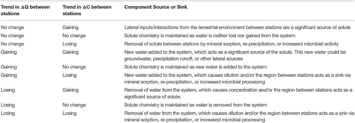
Table 1. Analysis and interpretation of differential concentration-discharge relationships.
To further evaluate the advantages of using differential concentration-discharge (ΔC- ΔQ) relationship in comparison to other approaches, Figure 1 depicts the characteristic features of traditional and differential C-Q relationships for a hypothetical solute sampled at an upstream station A and a downstream station B. Figure 1A demonstrates the seasonal variability in solute concentration and its corresponding relationship to stream discharge using the traditional C-Q analysis. Here, the direction of hysteresis loops can be used to infer the timing and mixing of various source waters (e.g., Evans and Davies, 1998; Carroll et al., 2007; Ward et al., 2013). For example, the hypothetical solute demonstrates negative counterclockwise hysteresis at station A implying that higher concentrations are observed on the falling than the rising limb at this location. In contrast, the hypothetical solute demonstrates a negative clockwise hysteresis at station B suggesting that that higher concentrations are observed on the rising than the falling limb at this location. When used in combination with hysteresis indices or mixing models, these C-Q hysteresis patterns can be further used to infer the relative contribution of different sources (e.g., Evans and Davies, 1998; Rose, 2003; Aich et al., 2014). In comparison, logarithmic C-Q analyses (Figure 1B) provide information about the overall variability in solute concentration (Godsey et al., 2009; Musolff et al., 2015; Bieroza et al., 2018). In particular, a slope essentially equal to 0 in log-log plot defines chemostatic behavior, or where concentration remains constant as discharge varies (Godsey et al., 2009; Wymore et al., 2017). In contrast, a negative (or positive) slope suggests a chemodynamic behavior corresponding to dilution (or concentration) of the solute at that location. The log-log plot here indicates that the hypothetical solute shows dilution with increasing discharge at both stations A and B, albeit to different degrees. Although recent availability of high-frequency data sets are expanding the scope and application of these techniques (e.g., Rose et al., 2018; Knapp et al., 2020), log-log plots are typically applied to long time-frame datasets and are used to compare solutes across different catchments, while standard C-Q relationships are typically used to study solutes intensively at one station with temporal differentiation. More importantly, both the standard and logarithmic C-Q relationships provide solute behavior characteristics at a single location within a stream.

Figure 1. Comparison of concentration-discharge analyses for a hypothetical solute at hypothetical stations A (upstream) and B (downstream) using (A) actual C-Q, (B) log C- log Q, and (C) ΔC- ΔQ. Arrows in (A) indicate direction through time; gray diagonal lines in (B) represent a log-log slope of −1 indicating dilution and blue lines show linear fits; a red “no change” line is shown in (C) demarcating gains from losses in solute turnover.
In contrast, differential C-Q relationships can provide insights on temporal and spatial variability in solute concentration across river segments (as delineated by different sampling stations). In addition, it provides information on the change in concentration within a specific interval of the river system, and thus on the applicable source or sink term. This technique can be particularly useful in identifying stream sections that are hot spots of metals or harmful solutes as well as the timing of when these hot spots occur. For example, Figure 1C suggests that the difference between solute concentration at station B and station A is >0 during the rising limb period, while it is negative during the base flow period. This indicates that the solute accumulates within the segment between stations A and B during the rising limb period, while it is diluted during the base flow period. For a harmful chemical, the rising limb period would be the time where monitoring or best management practices may be needed to bring down the concentration to an acceptable level. A negative difference in concentration across stations during the falling limb period, which increases with increasing discharge, suggests that the solute concentration is decreasing due to reactions, sorption or other biogeochemical processes within the river segment during this time period.
Field Site and Datasets
Study Site
To evaluate and compare differential C-Q approach with traditionally used approaches in understanding solute behavior, we focus on water quality data available for three sampling stations within the East River Catchment. The East River Catchment, described in detail in Hubbard et al. (2018), is located in Gunnison County near the town of Crested Butte, Colorado (Figure 2). The East River contributes approximately 25% of water to the Gunnison River, which is an important tributary of the Colorado River (Battaglin et al., 2012). Given that by mid-21st century the population utilizing this water is expected to increase by 50–100% while streamflow is expected to decrease by 20% (Udall and Overpeck, 2017), the East River flow and its runoff components are important to characterize and catalog for downstream users of the Colorado River.
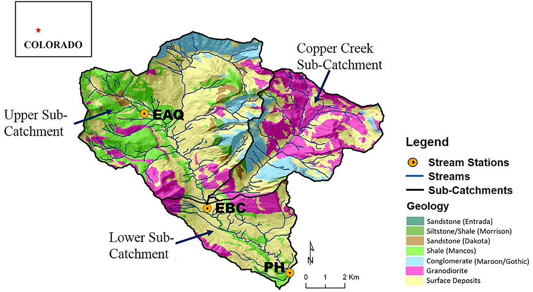
Figure 2. Location of the East River Catchment, CO, USA overlain on a bedrock geology map showing the monitoring stations and the sub-catchments that are the focus of this study. The upstream reach is defined as the segment between EAQ and EBC, and the downstream reach is defined as the segment between EBC and PH. EAQ, East Above Quigley; EBC, East Below Copper; and PH, Pump House.
The East River watershed covers an approximate area of 84 km2 with an average elevation of 3,350 m (Winnick et al., 2017). The East River hydrologic cycle (Figure 3) is dominated by snowmelt in spring and early summer months, with monsoonal rain being significant in early-to-late summer months (Markstrom et al., 2012; Winnick et al., 2017). The geology of the watershed is comprised of a diverse collection of Paleozoic and Mesozoic sedimentary rocks intruded by Tertiary igneous laccoliths and ore-rich stocks (Dwivedi et al., 2018b; Hubbard et al., 2018). Cretaceous Mancos Shale forms the primary bedrock of the study site (Figure 2). Mancos Shale in this region is associated with elevated carbon, metal and pyrite content, and its weathering can thus significantly affect water quality (Morrison et al., 2012; Kenwell et al., 2016).
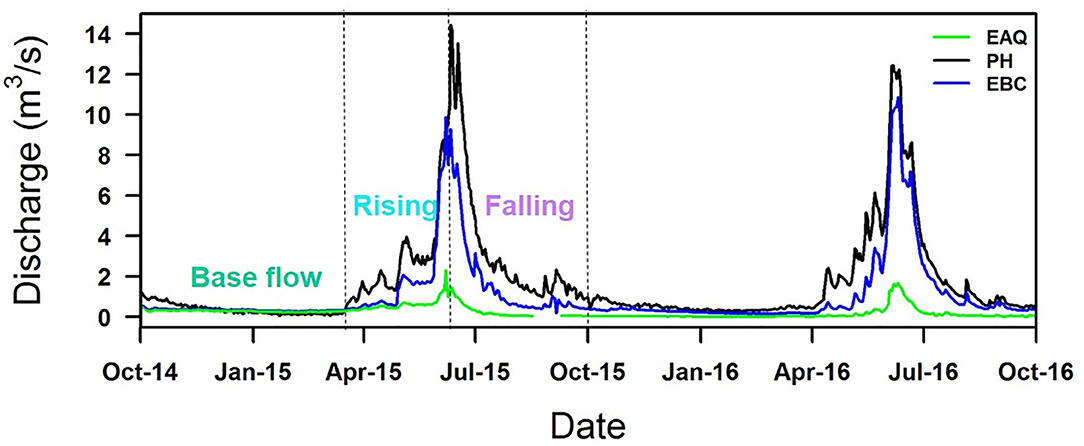
Figure 3. Discharge rates measured at East Above Quigley (EAQ), Pump House (PH), and East Below Copper (EBC) stations for two consecutive water years. Discharge represents distinct seasonal trends, being higher in snowmelt-dominated spring months than in winter. Note that the C-Q relationships were analyzed on the basis of the discharge graph separation into base flow, rising and falling limb components as shown here.
Climate at the East River is characterized by long, cold winters and short, cool summers (Hubbard et al., 2018). The mean annual air temperature and annual precipitation (1981-2017) at the site are 2.12°C and 673 mm, respectively. Precipitation occurs in the form of rainfall between July and September, with June being the driest month. Snow accounts for about 64% of the precipitation (Pribulick et al., 2016). Snowmelt typically begins in early April and freeze-up occurs in late November. Vegetation at the site consists primarily of four community types—sagebrush, spruce-fir, upland-herbaceous, and alpine (Zorio et al., 2016).
Streamflow Sampling and Chemical Analyses
Stream samples and discharge measurements were collected for multiple consecutive water years (2015–2018) at three stream gauging stations—East Above Quigley (EAQ), East Below Copper (EBC), and Pump House (PH) (Figure 2). These data are available online at http://dx.doi.org/10.21952/WTR/1495380. Among these stations, EAQ drains water from a basin with medium elevation, medium relief and steep slopes, while EBC drains water from the entire upper basin with overall higher elevation and higher relief features (Table 2). An important difference between the stations is that streamflow at EAQ originates from the upper sub-catchment that is primarily underlain by Mancos Shale, while at EBC, a significant proportion of the flow originates within an igneous cirque composed of quartz monzonite and granodiorite from which it then traverses sedimentary strata. In comparison, PH is located in the low-relief meandering floodplain section of the East River that is eroding primarily into the Mancos shale. These three sampling stations were chosen for this study because they are representative of the topographically complex terrain of the East River catchment and reside directly along the main East River tributary.
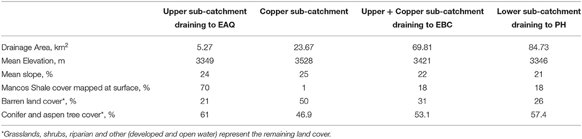
Table 2. Characteristics of sub-catchments in the East River Watershed relevant to this study (modified from Carroll et al., 2018).
At all sampling stations, instantaneous stream discharge measurements were made using SonTek Flow Tracker® acoustic Doppler velocimeter (Winnick et al., 2017; Carroll et al., 2018). The discharge characteristics for the entire duration of the study period are shown in Figure 3. The pattern of discharge is quite consistent from year to year, although the scale may vary from one year to the next. In particular, EAQ had the lowest discharge values, while EBC and PH had comparable values. In this study, discharge measurement collected with a paired geochemical data are only reported.
Geochemical analysis of all instream samples includes Ca, Cl, Cu, dissolved inorganic carbon (DIC), dissolved organic carbon (DOC), Fe, K, Mg, Mo, Na, NO3, P, Si, and SO4. Detection limits and estimated relative standard deviation for each solute is provided in Table S1. Instream samples for geochemical analysis were collected daily using automatic sampler (Model 3700; Teledyne ISCO, NE, USA) via a peristaltic pump at PH, while water samples were collected in-situ at EBC and EAQ stations at bi-weekly to monthly frequencies. All samples were filtered in the field using 0.45 μm Millipore filters. Anion samples were collected in no-headspace 2 mL polypropylene vials. DIC/DOC samples were collected in no-headspace 40 mL glass vials with polypropylene open-top caps and butyl rubber septa (VWR® TraceClean®). Cations samples were collected in high-density polyethlene 20 mL vials and acidified to 2% nitric acid with ultra-pure concentrated nitric acid. The samples were transported to the laboratory on ice and stored in 4°C refrigerator until analysis. Anion concentrations were measured using a Dionex ICS-2100 Ion Chromatography (IC) system (Thermo Scientific, USA), while cation concentrations were analyzed using an inductively coupled plasma mass spectrometry (ICP-MS) (Elan DRC II, PerkinElmer SCIEX, USA) (Carroll et al., 2018). DIC and DOC concentrations were measured using a TOC-VCPH analyzer (Shimadzu Corporation, Japan). DOC was analyzed as non-purgeable organic carbon (NPOC) by purging acidified samples with carbon-free air to remove DIC prior to measurement. Further details on sampling and measurement methods are described in detail elsewhere (Williams et al., 2011; Dong et al., 2017).
Note that paired upstream C-Q and downstream C-Q data are needed for differential C-Q analysis. Therefore, the requirement of data for ΔC-ΔQ is much larger than traditional analyses. Because sampling frequency differed by station type, sample size varied between 234 and 1,164 observations with lowest frequencies associated with solutes at EAQ. Even with these limited data, the results of this study highlight the value of using differential C-Q analysis in spatially characterizing solute behavior within a watershed. Moreover, the sampling spanned over 90% of the flow regime, indicating good representation of flow conditions.
Concentration-Discharge Metrics
We compared the differential C-Q technique with commonly used C-Q metrics to identify what new information, if any, can be obtained from the new differential technique that is not apparent from these metrics with respect to lateral transport, mixing and reaction processes. For this purpose, concentration-discharge relationships were assessed using three metrics: (1) logarithmic concentration- logarithmic discharge (log-log), (2) actual concentration -discharge (C-Q), and (3) differential concentration-differential discharge (ΔC- ΔQ).
First, we plotted the concentrations of each of the major solutes against discharge on logarithmic axes of equal units. Assuming a power law relationship of the form C = aQb, the best-fit slope b of the log-log plot was used to describe chemostatic or chemodynamic behavior (Godsey et al., 2009). As suggested above, a slope of 0 indicates chemostatic behavior—i.e., the solute remains at a constant concentration despite changes in discharge—and therefore, discharge is not considered to be the dominant control. A slope of −1 indicates solute concentration dilutes with discharge and a slope of +1 indicates solute concentration increases with discharge; both of these relationships are dependent on river discharge and demonstrate chemodynamic behavior. Student's t-test was further used to determine whether the best-fit slopes were significantly similar to reference slopes of 1, 0, or −1 (Godsey et al., 2009; Wymore et al., 2017). However, C-Q patterns can be more complex and need not adhere to these simple slopes of 1, 0, or −1. To identify such solutes, we examined residual data points about the best-fit line; those with large ranges in concentration and low coefficients of determination (R2) do not have a power law relationship and are classified as such (Thompson et al., 2011; Moatar et al., 2017; Bieroza et al., 2018).
Second, we used plots of solute concentration vs. discharge to determine hysteresis patterns and seasonal trends. Hysteresis patterns signify the difference in solute concentration on the falling and rising limb of the C-Q plot at the same value of discharge (Williams, 1989; Gellis, 2013). The extent and degree of hysteresis depends on different catchment pathways activated and the mixing of different source waters. An examination of the hysteresis patterns can therefore provide information regarding different transit times and the differing contribution of solutes to the stream from various water sources (Evans and Davies, 1998; Lloyd et al., 2016). In this study, hysteresis categories were based on Hamshaw et al. (2018), who expanded on the original classes proposed by Williams (1989). Four hysteresis patterns were found to commonly persist: (1) clockwise hysteresis with higher concentrations on the rising than the falling limb, (2) counterclockwise hysteresis with higher concentrations on the falling than the rising limb, (3) figure-eight configuration with higher concentrations on the rising than the falling limb for a certain range of Q values and lesser concentrations for other Q values, and (4) type-1 where C/Q ratio on the falling and rising limbs fall on a single-valued line. Additionally, a distinction is made with the figure-eight configuration that typically follows a counterclockwise pattern first and then becomes clockwise. In contrast, a figure-then-counterclockwise hysteresis pattern occurs when an initial solute concentration is followed by a delayed release (Gellis, 2013). Furthermore, each of these C-Q plots can be used to determine if solute concentration is consistently higher at base flow than at other times, or if rising or falling limb concentrations are greater than base flow concentration. In this study, the variable source contributions were interpreted based on the framework proposed by Evans and Davies (1998). Evans and Davies (1998) in a benchmark paper presented a unique relationship between the form of C-Q hysteresis loops and variable contributions of two- and three-component mixtures. Here, a three-component mixing model comprised of ground water (GW), soil water (SW), and event water (SO) was deemed appropriate based on prior work (Carroll et al., 2018). These hysteresis patterns thus provide important information regarding the prevalence of event, soil and ground water, and dynamic watershed interactions at different times.
Lastly, ΔC- ΔQ was obtained as the difference in concentration in a river segment over the difference in discharge across the same segment over the same time period (adjusted by the time to peak at individual stations). As shown in Figure 3, the hydrograph peaks were coincidental for EAQ and EBC stations, while the difference in hydrograph peak at PH was 1 day. These plots were interpreted according to Table 1.
Results and Discussion
Analysis of Log-Log Relationships
Table 3 displays the log-log trends for all solutes at EAQ, EBC, and PH stations. In this table, each geochemical species is assigned a chemostatic/chemodynamic classification and a slope based on where the data points lie within the logarithmic space. As described in the previous section, logarithmic C-Q slopes can be defined if the relationship between the solute and river discharge at the target location is linear, i.e., if a power-law relationship exists, and these linear slopes can be positive, negative, or neutral. For power-law relationships with significant variability in concentration values such that the |slope| is > 0.1, solutes are considered to be chemodynamic (Godsey et al., 2009; Bieroza et al., 2018).
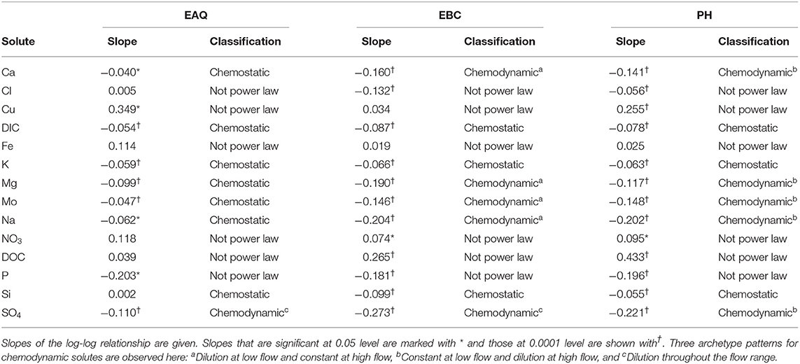
Table 3. Log- log relationship for solutes at all three stations of the East River watershed.
For a majority of the solutes in this study (24 out of 42), logarithmic concentration-discharge relationships are linear, suggesting that a power-law relationship exists between concentration and discharge at these sampling stations. For these solutes, the slope parameter ranged between −0.273 and 0.002 across all sites and solutes. This indicates that most of these solutes have a constant or negative relationship with discharge. Further, a p-value of 0.05 and 0.0001 is used to signify the strength of this relationship. In contrast, certain solutes Cl, Cu, Fe, NO3, DOC, and P, have a wide range in concentration with most residual data points lying well outside the best-fit slopes of either 1, 0, or −1. Moreover, the coefficient of variation ratios (CVC/CVQ) for these six solutes ranged from 0.61 to 3.73, while the corresponding values for Ca, Mg and Na ranged from 0.06 to 0.28. Therefore, the higher ratios and lower R2-values (≤0.28) suggest that the power law equation alone is insufficient to describe the C-Q relationship for these six solutes. It is interesting to note that a few of these non-conforming solutes (Cu, Fe, NO3, DOC) showed a positive slope indicating enrichment of these solutes with increasing discharge.
Table 3 further shows that three solutes (DIC, K and Si) consistently demonstrated chemostatic behavior (|slope|<0.1) across all stations. This implies that these solutes either have a uniform distribution within the catchment or that changes in hydrologic connectivity and flow paths within the catchment do not affect the concentration or production of these solutes (Godsey et al., 2009; Moatar et al., 2017). With the exception of these three, all other solutes showed chemodynamic behavior at the Pumphouse (PH). Among these, solutes that conformed to the power-law relationship demonstrated stable patterns at low flow conditions and dilution during high flows (Figures 4, 5). These solutes are considered to be source-limited since delivery to the stream network is controlled by their rate of production as opposed to transport-limitation (Meybeck and Moatar, 2012; Bieroza et al., 2018). Both redox-sensitive solutes (e.g., Mo, SO4) as well as weathering-related solutes (e.g., Ca, Mg, Na) demonstrated source-limitation at PH. While chemodynamic behavior of redox-sensitive and biogeochemically active solutes is commonly observed, chemodynamic behavior of weathering-based ions has also been reported in some carbonate-dominated catchments (e.g., Sullivan et al., 2018). This is usually attributed to spatial heterogeneity, activation of different flow paths and/or mineral control (Koger et al., 2018; Rose et al., 2018; Molins et al., 2019; Knapp et al., 2020). At PH, sulfuric acid weathering is estimated to account for 35–75% carbonate dissolution (Winnick et al., 2017), thus resulting in source-limitation of weathering solutes at this location.
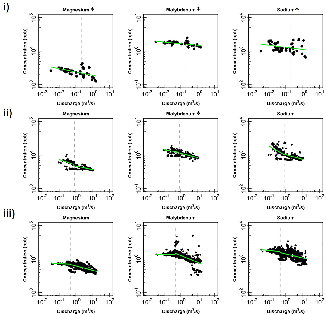
Figure 4. Change in log-log relationships for Mg, Mo and Na at (i) EAQ, (ii) EBC, and (iii) PH when segmenting the hydrograph at the median discharge (dashed gray line). Low flows indicate values below the median discharge and high flows indicate values above the median discharge. Green lines represent segmented linear fits to the data, and * indicates if slopes at low and high flows are significantly similar to each other at 0.10 level.
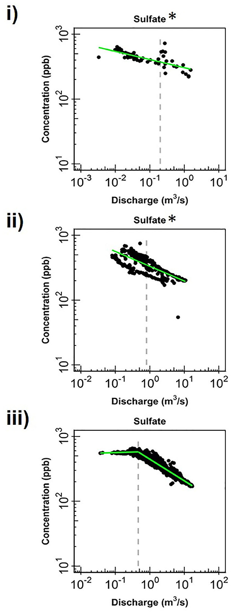
Figure 5. Change in log-log relationships for SO4 at (i) EAQ, (ii) EBC, and (iii) PH when segmenting the hydrograph at the median discharge (dashed gray line). Green lines represent segmented linear fits to the data, and * indicates if slopes at low and high flows are significantly similar to each other at 0.10 level.
Apart from the commonalities described above, most of the solutes at EAQ demonstrated chemostatic behavior. These include Mo as well as weathering-related solutes such as Ca, Mg and Na. Only SO4 showed chemodynamic behavior, with a negative slope parameter indicating dilution throughout the flow range (Figure 5).
At EBC, all solutes exhibited the same chemostatic and chemodynamic relationship as observed at the PH station. However, a major difference between the chemodynamic relationship at PH and EBC is that solutes at EBC showed dilution at low flow conditions and stabilization under high flow conditions (Figure 4). This was consistent for weathering-related solutes like Ca, Mg and Na as well as redox-sensitive species like Mo. Therefore, these solutes exhibited more variability in concentration at low flows at EBC, while at PH, these solutes demonstrated more variability at high flows. Furthermore, SO4 patterns at EBC showed dilution throughout the whole flow range, while SO4 at PH showed stabilization at low flow conditions (Figure 5).
Even though all three stations lie within the East River catchment, variability was observed in solute concentrations as well as their log-log behavior. In particular, weathering-related solutes showed chemostatic behavior at EAQ, and chemodynamic behavior at EBC and PH. These differences in the nature of C-Q relationship can be attributed to seasonal shifts in flow paths and variability in the fraction of base flow contribution that interacts with the weathered profile and ends up in the stream. Note that the fraction of groundwater contribution to the EAQ station varied by only 0.15 throughout the flow regime, while the variation for EBC and PH was much higher at 0.25 (Carroll et al., 2018).
Analysis of C-Q Hysteresis Patterns
Within the East River, discharge is highest during the spring months (the rising limb) and lowest during the winter months (base flow), as is typical for Rocky Mountain headwaters (Figure 3). These seasonal discharge patterns can cause hysteresis and influence solute concentrations. Solute concentrations across all stations were analyzed for three portions of the hydrograph: (1) base flow, (2) rising limb, and (3) falling limb. Hysteresis differences in solute concentrations between the rising and falling limb were also analyzed as shown in Table 4.
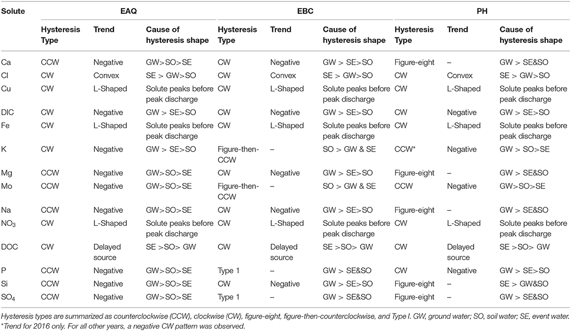
Table 4. Classes of hysteresis in concentration-discharge plots for solutes at all three stations of the East River watershed.
Table 4 indicates that most of the solutes (25 out of 42) exhibited clockwise (CW) hysteresis, where higher solute concentrations occur on the rising limb of the hydrograph and lower concentrations occur on the recessional limb (Wood, 1977; Williams, 1989; Gellis, 2013; Gwenzi et al., 2017). Causes for this hysteresis pattern have been explained primarily by an initial “flushing” of the solute and relative depletion during the falling limb. Table 4 further indicates that significant subcategories of the CW loop were obtained by discriminating between the loop direction. These subcategories can provide important insights about how transport mechanisms vary between solutes and through time. CW loops were observed in solutes across all stations. In contrast, only a small number of solutes (8 out of 42) showed counterclockwise (CCW) behavior (Table 4). CCW behavior has been explained by a solute peak arriving later than the discharge peak, such that there is a delayed source or lagged “through-flow” response contributing to higher concentration on the falling than the rising limb of the hydrograph. For the CCW loops, all except one were sampled at EAQ. Table 4 further indicates that all CCW loops had a negative trend.
Both EBC and PH featured significant diversity in hysteresis types, including occurrences of figure-eight and figure-then-counterclockwise patterns. Figure-eight hysteresis is observed when C/Q ratios on the rising limb for some discharge values are greater than those on the falling limb for the same discharge values. In the latter, C/Q ratios on the rising limb for some discharge values are smaller than those on the falling limb for the same discharge values, with the distinction that the initial solute concentration is followed by a delayed release. Both figure-eight and figure-then-counterclockwise hysteresis loops are indicative of distinct solute sources that become activated at different times during the year (Megnounif et al., 2013).
Patterns exhibiting no hysteresis (Type 1) were also observed, although these occurred relatively infrequently (2 out of 42) and were noted only at EBC. Type 1 patterns occur when there is a systematic variation in solute concentrations with discharge (Murphy et al., 2014). We demonstrate the different C-Q patterns observed within the East River watershed using specific examples from the sampling stations (Figure 6).
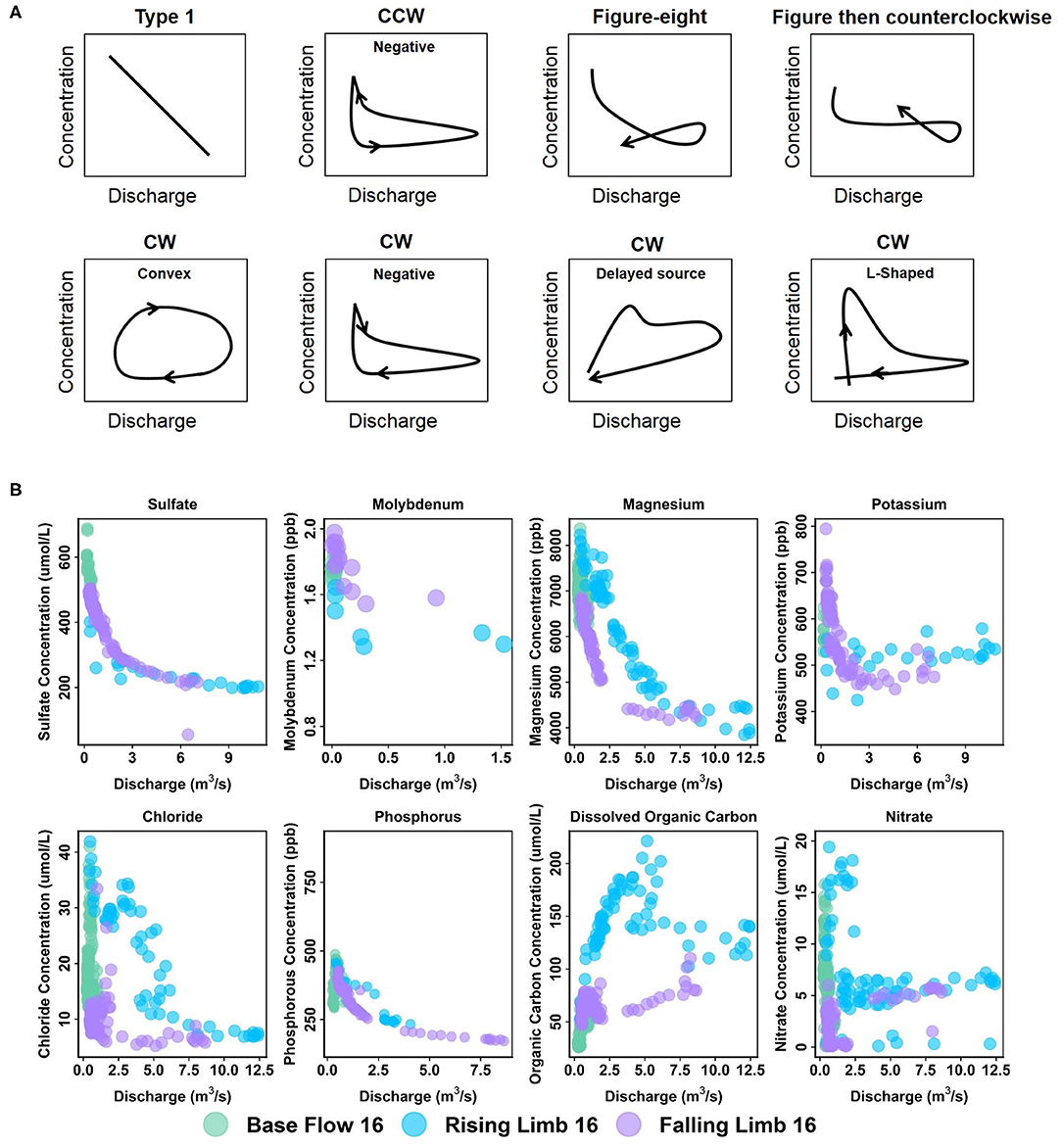
Figure 6. (A) Types of C-Q patterns commonly observed at the East River Catchment, and (B) example of solutes from different stations demonstrating these patterns. Arrows in (A) indicate direction through time. C-Q plots of K and SO4 correspond to EBC, Mo to EAQ, and the rest to PH.
At EAQ, seven solutes (Cl, Cu, DIC, DOC, Fe, K, and NO3) exhibited clockwise hysteresis and an equal number of solutes (Ca, Mg, Mo, Na, P, Si, and SO4) exhibited counterclockwise hysteresis. As suggested above, only negative counterclockwise loops were observed. This implies that for these solutes, groundwater contributions were greatest at this location, followed by soil water contributions, and then surface runoff. For the clockwise loops, trends at EAQ varied significantly between solutes. DIC and K had negative clockwise hysteresis, such that groundwater contributions still dominated the C-Q behavior, but event water contributions were greater than soil water contributions. In contrast, DOC exhibited a clockwise loop with an irregular pattern. This loop is characterized by an early, rapid increase in DOC concentration during the rising limb, followed by a delayed, second pulse of DOC concentrations. The second pulse is typically attributed to a slow contributing source or late activation of certain flow paths. At the East River, these pulses can be attributed to shallow soil horizon DOC concentrations that are rapidly mobilized by spring snowmelt, and deeper groundwater DOC contributions that are lagged because of the progressive infiltration of snowmelt. This loop is similar to Type 2E reported in Hamshaw et al. (2018). Unique C-Q relationships were also demonstrated by Cu, Fe, and NO3, which showed an L-shaped clockwise hysteresis. This implies that a peak in solute concentration occurred before the peak in discharge. This can potentially occur due to fast release or flushing of old water with high solute concentration. Such loops were characterized as Type 2D by Hamshaw et al. (2018) and were most frequently observed in the rainier summer and early Autumn months. Here, significant concentration of these metals and nitrate are attributed to the underlying Mancos Shale (Deacon and Driver, 1999; Morrison et al., 2012).
Unlike EAQ, half of the solutes at PH exhibited clockwise hysteresis (7 out of 14), five solutes showed a figure-eight configuration, and two exhibited counterclockwise hysteresis. Except P, all solutes that showed clockwise hysteresis (Cl, Cu, DIC, DOC, Fe, and NO3) at PH had trends that mirrored those observed at EAQ. P was found to demonstrate consistently different patterns across stations. However, it is notable that groundwater contributions were greatest for P across stations, while soil water and event water contributions varied. At PH, the figure-eight loops were specifically observed for Ca, Mg, Na, DIC, Si, and SO4. As suggested above, this could be related to a variety of factors such as variable source area contributions or the relative difference between concentration and discharge peaks. One notable exception to the clockwise and figure-eight loops observed at PH was Mo, which showed a counterclockwise hysteresis loop. However, similar to EAQ, it had a negative trend such that groundwater contributions were greatest, followed by soil water, and then event water contributions. Mo deposits are also attributed to the underlying geology at this site (Deacon and Driver, 1999; U.S. Department of Energy, 2011). Note that K is the only element that displayed different hysteretic patterns for 2016 at PH than other years and shows a CCW trend as opposed to the typically observed CW pattern. This suggests that in a typical year, snowmelt event water is the secondary source of K to the stream, but in 2016 subsurface soil water was the secondary source of K. This seems reasonable because 2016 had lower than average precipitation.
Across all stations, only six solutes showed consistent behavior in their C-Q patterns. These include Cl, Cu, DIC, Fe, NO3, and DOC, all of which exhibit clockwise hysteresis. Two other solutes with clockwise hysteresis—Mo and K—displayed similar behavior across EAQ and PH, but different from those observed at EBC. Interestingly, weathering-related solutes and P showed consistently different patterns across all stations. At EBC, weathering-related solutes including Ca, Mg, and Na showed a negative clockwise hysteresis. As suggested above, this implies that groundwater contributions were greatest, followed by surface runoff, and then soil water. Two notable exceptions observed at EBC were the Type 1 pattern shown by P and SO4, and the figure- then-counterclockwise hysteresis exhibited by K and Mo. While Type 1 is indicative of a consistent source or source area contributions to the solute concentrations sampled at EBC, the figure-then-counterclockwise hysteresis is typically a result of distinct sources or variable source area contributions. The steep slopes, high relief and convergent topographic features of EBC can result in an uninterrupted supply of certain solutes such as P and SO4. Carroll et al. (2019) also noted that recharge in the Copper Creek sub-catchment appears to be decoupled from annual climate variability, resulting in a steady supply of certain solutes.
Analysis of ΔC- ΔQ Patterns
Solute data in the upstream and downstream reaches of the East River watershed were analyzed through ΔC- ΔQ analysis to evaluate storage mechanisms and lateral connectivity. The increase in discharge was on average 0.22% of the absolute discharge (range 0.01 to 2.06%) between EAQ and EBC (i.e., the upstream reach) and at 0.12% (range −0.07 to 0.92%) between EBC and PH (i.e., the downstream reach). Because EBC is a tributary junction (see Figure 2), larger increases in discharge are observed in the upstream than the downstream reach. The range of discharge values further demonstrate that both upstream and downstream reaches were generally gaining during the study period. Only for a few times during the base flow period does the downstream reach become a losing stream (not shown here). The fraction of solute gained or lost within a given reach varied with change in discharge.
Figure 7 shows the ΔC- ΔQ relationships for a subset of solutes in the downstream reach for 2015 and 2016 water years. A complete description of the differential C-Q relationships for all years (2015–2018) is shown in Table 5. For ease of interpretation of results from Figure 7, we present an example wherein Ca is the solute of interest. We note that both gains and losses of Ca are obtained when the difference in discharge between stations is small (~0). Although overall gains in discharge are small, the stream is not a pipe and significant stream water-groundwater interactions are expected within this focus floodplain section. Here, the downstream reach shows a loss (negative concentration) of Ca during the rising limb, while it shows a gain (positive concentration) for most of the falling limb, especially with higher ΔQ values. Spring snowmelt is an important contributor to the streamflow during the rising limb and can dilute Ca concentration. Note that other processes may also contribute to a decline during the rising limb, such as gypsum precipitation or ion exchange. However, the effect of these processes may be small in comparison to the significant dilution obtained due to snowmelt. For the increase in concentration noted during the falling limb, it is possible that these sources were generated at the far end of the contributing area, and thus Ca reaches the stream mainly during the falling limb. Overall, the downstream reach between EBC and PH shows a net increase in Ca specifically during periods of high gains in discharge. This trend is noted in Table 5 documenting Ca behavior at both low and high ΔQ values. It is interesting to note that Mo and K show a behavior similar to Ca, except that K shows net losses with higher ΔQ (Table 5). The main reason for this is that losses in K are observed during the falling limb of 2015, while gains are observed during the falling limb of 2016 (Figure 7B). This inconsistency is due to the fact that 2015 had greater total precipitation, which mainly came from a larger proportion of summer monsoon (30%) than observed in 2016 (26%). Because significant uptake of K can occur by plants, microbes or both, that are typically triggered by moisture conditions, these monsoon events led to a noticeable decline in K during 2015, but not in 2016.
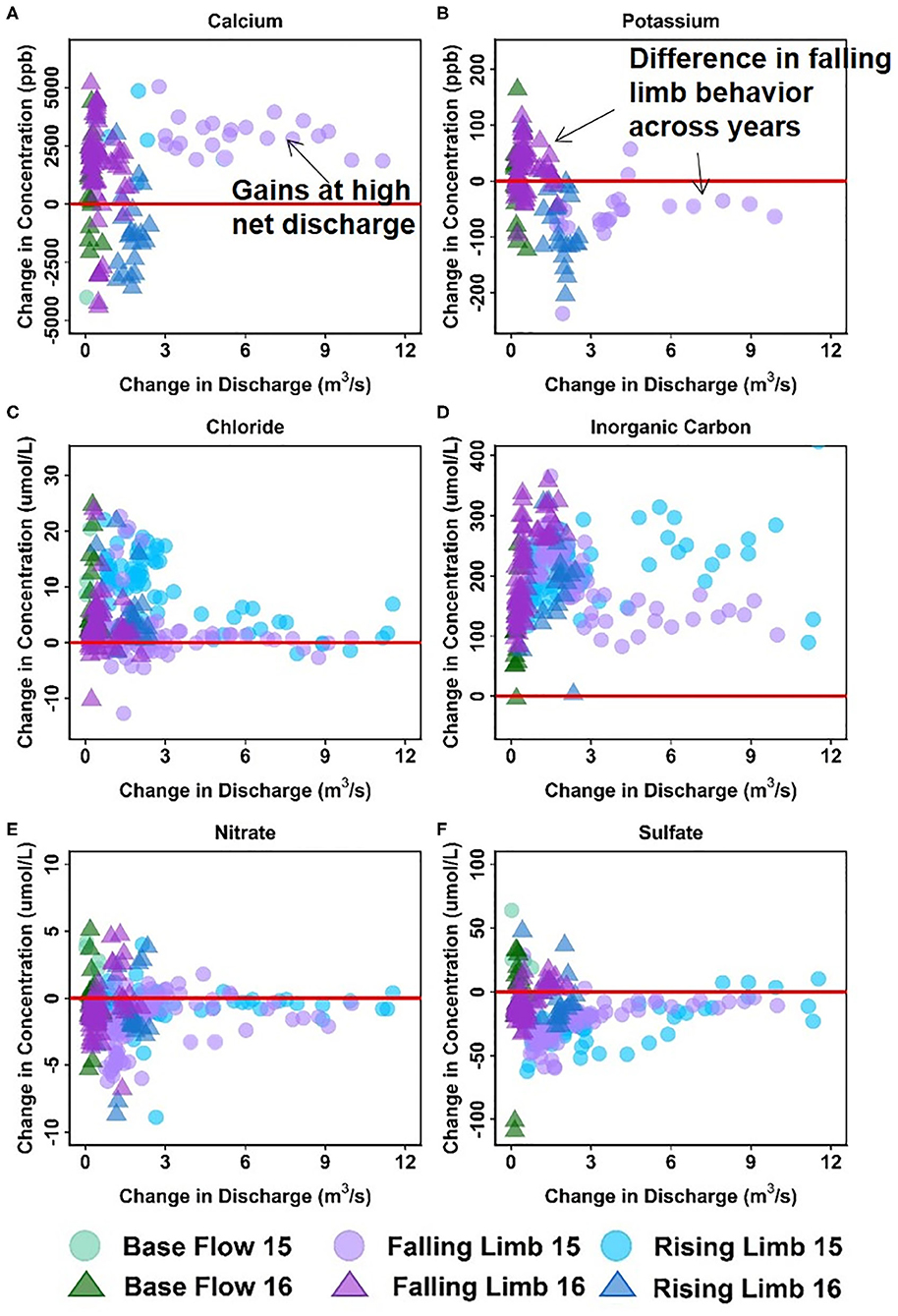
Figure 7. Differential C-Q analyses for the downstream reach showing changes in concentrations of (A) Ca, (B) K, (C) Cl, (D) DIC, (E) NO3, and (F) SO4 relative to changes in flow. For clarity, gains and losses of solutes are demarcated relative to a solid red “no change” line.
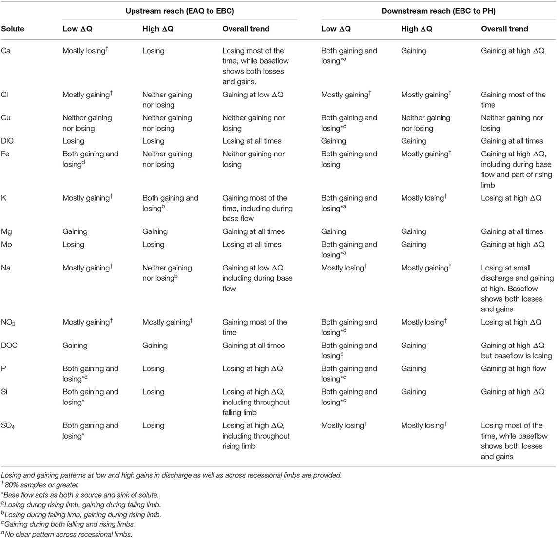
Table 5. Differential concentration-discharge relationship for solutes at the upstream and downstream reaches of the East River watershed.
Table 5 further indicates that most solutes (9 out of 14) showed net gaining trends or increases in concentration in the downstream reach. This is reasonable given the low relief meandering nature of this section of the East River. Among these, Cl, DIC, and Mg showed a consistent increase in concentration throughout the hydrograph (see, for example, Figures 7C,D). This implies that lateral contributions are significant in this focus floodplain section and add to the stream concentrations of these solutes. Tokunaga et al. (2019) confirm that hillslope contributions to PH are significant and typically contribute to 54–57% of solute exports. In comparison to these solutes, DOC, P and Si showed a gain in concentration at all times except the base flow period. This suggests that base flow is not a significant source of these solutes or that surficial soils and shorter flow paths are important sources that are able to increase or maintain their concentration in the stream. Last but not least, Fe showed a gaining trend within this reach, especially at high ΔQ values. At low ΔQ values, base flow and portions of rising limb showed gains in Fe, while the falling limb acts as both a source and sink of Fe. In their study, Wan et al. (2019) noted that water table fluctuations drive pyrite weathering in Mancos shale environments. Thus, gains in Fe are possibly associated with pyrite oxidation, while the losses during the falling limb may be attributed to chemolithoautotrophic microbial reactions, mineral precipitation or other processes that consume Fe (Arora et al., 2015, 2016).
Only three solutes showed a decline in concentration within this reach. In particular, SO4 showed a consistent loss, while K and NO3 showed losses at high ΔQ only. For both sulfate and nitrate, a gain in concentration was observed for most of the base flow period, while a loss was observed for most of the rising and falling limb (Figures 7E,F). This suggests that ground water is a significant source of sulfate and nitrate, while spring snowmelt and microbial reactions result in a decline of these concentrations. Cu and Na showed unique trends within this reach (Table 5). Na, in particular, showed losses at low ΔQ values and gains at high ΔQ. Further, gains in Na were only observed in 2015 and losses were limited to 2016. It is well known that rainfall is an important source of Na and Cl (Junge and Wurbe, 1958). Given that 2016 had lower than average rainfall while 2015 had a greater percentage of precipitation falling as summer rain, it is reasonable that we observed an increase in Na concentration only in 2015. Chloride concentrations, on the other hand, showed gains at both low and high ΔQ values. This is because deep groundwater is also a source of chloride in this segment of the river. In contrast to Na and Cl, Cu showed neither gains nor losses within this reach. A similar trend for Cu was also observed in the upstream reach.
Apart from Cu, Mg is the only other solute that showed consistent trends across the reaches (Table 5, Figure 8A). In fact, most solutes (7 out of 14) in the upstream reach showed trends opposite to those observed in the downstream reach. For example, DIC shows an overall losing trend within the upstream reach as opposed to an accumulation within the floodplain (Figures 7D, 8B). Similar to DIC, solutes such as Ca, Mo, P, and Si also switched from losing trends in the upstream reach to gaining trends in the downstream reach (see, for example, Figure 8C). Because EBC is a tributary junction assimilating flows from both EAQ and Copper Creek, the gross loss of a solute can imply that concentration at EAQ is higher than at Copper Creek or combined flow at EBC. Further note that EAQ captures the solute turnover from most of the upper catchments in the East River that have a higher fraction of basin area underlain by Mancos Shale (0.70) as compared to Copper Creek (0.01) (Carroll et al., 2018). Thus, most of the losing trends in the upstream reach are observed in geogenic elements associated with Mancos shale (e.g., DIC, Ca, Mo). In contrast, the downstream reach is defined by a low-energy meandering floodplain that is eroding primarily into the Mancos shale, which is composed of quartz, feldspar, interbedded clays, carbonates, and pyrite (Gaskill et al., 1991). Thus, gains in these geogenic solutes are observed in the downstream segment. Table 5 further suggests that only K and NO3 switched from gaining trends in the upstream section to losing trends in the downstream section (Figures 7E, 8D). Given the ~11 km long meanders in the downstream reach that offer significant area for lateral interactions and microbial uptake (Dwivedi et al., 2017, 2018b), it is reasonable that we observed a decline in reactive elements like K and NO3. Taken together, most solutes (6 out of 14) showed losses within the upstream reach, with 50% of these solutes showing losses only at higher ΔQ values. In contrast, gains were limited to geogenic and runoff-derived solutes such as K, Mg, NO3 and DOC. Sodium and chloride gains were limited to low ΔQ suggesting similar processes (e.g., rainfall) impacting their turnover. Only trace metals like Cu and Fe showed neither gains nor losses within this reach.
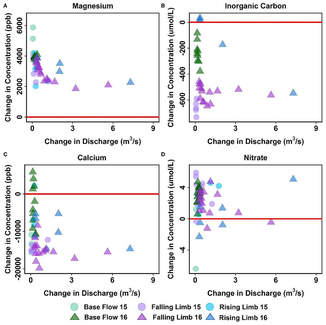
Figure 8. Differential C-Q analyses for the upstream reach showing changes in concentrations of (A) Ca, (B) DIC, (C) Mg, and (D) NO3 relative to changes in flow. For clarity, gains and losses of solutes are demarcated relative to a solid red “no change” line.
Comparison of ΔC-ΔQ to Other Studies and Implications
Capturing solute turnover across stream segments has important implications for water and land management applications such as nutrient transport, contaminant transport, and developing pollution prevention/intervention strategies. Previous studies have used transient storage models to simulate solute tracer movement, stream water-ground water exchange, and interpret downstream solute transport (Payn et al., 2009; Covino et al., 2011; Ward et al., 2013). While transient storage models have provided a useful context for quantifying stream water balance, these models are constrained by the use and interpretation of recovered tracer breakthrough curves. These models can therefore miss longer recovery times and underestimate lateral exchange from stream segments. Studies by Szeftel et al. (2011) and Ward et al. (2013) further suggest that discharge alone is a poor predictor of gross gains and losses across stream reaches and can complicate transient storage interpretations by adding uncertainty to model parameters. Work is still underway in developing new experimental techniques (e.g., heat tracing) and advanced process representation (e.g., reactive transport models) to improve mechanistic understanding of solute behavior at stream water-ground water interfaces (Krause et al., 2014; Dwivedi et al., 2018a; Arora et al., 2019a). In this regard, the differential C-Q analysis presented here provides an easy-to-use tool to investigate the fractional solute turnover as a function of water gains and losses over each stream segment. Although stream segments are defined by sampling locations, smart pairing of these locations for ΔC-ΔQ analyses can provide an integrated measure of lateral transport and biogeochemical processing across multiple segments. By following a different spatial scheme and organizing the river into multiple sections, ΔC-ΔQ can provide a rapid assessment of the proportional influences of hillslope contributions to stream water composition and aid in identifying stream segments that are vulnerable to change. Further, ΔC-ΔQ analysis can evaluate solute turnover at a range of flow conditions. At the East River site, smaller gains in solutes were typically confined to base flow conditions, while larger gains across upstream and downstream segments were associated with rising limb and snowmelt periods (e.g., Figures 7, 8). Thus, this C-Q analysis is a valuable tool that can account for the specific sources, hillslope contributions and critical stream segments that can adversely impact instream concentrations.
Summary and Conclusions
Managing freshwater resources is proving difficult and exposes gaps in our scientific understanding of hydrological and biogeochemical processes controlling stream concentrations of solutes, trace metals and nutrients. To address this scientific and management need, we proposed a new differential C-Q analyses that identifies stream segments accumulating harmful chemicals under specific flow conditions. Hydrochemical data collected over 4 years in the headwaters of the Colorado River were analyzed through several C-Q metrics.
Log-log metrics demonstrated mostly negative relationships indicating that dilution is a primary mechanism controlling C-Q behavior within the ER watershed. Only a few solutes (DIC, K, Si) showed a discharge-invariant (chemostatic) behavior that was consistent across stations. Most solutes at EBC and PH showed chemodynamic behavior with two linear components at median Q values. Specifically, solutes at EBC showed more variance at low Q values and stability at higher flows, while solutes at PH showed greater variance at high flows and stability at low flows. In contrast, chemodynamic solutes at EAQ demonstrated highly linear trends and lacked the breakpoints or threshold behavior evident at other stations.
C-Q relationships showed that the most commonly observed hysteresis types were clockwise patterns indicative of a flushing behavior that causes a spike in solute concentration to occur before peak discharge. Counterclockwise patterns occurred less frequently and were more commonly observed at EAQ, indicative of distant sources or delayed mobilization. Hysteretic behavior suggestive of multiple sources and variable source area contributions was observed at both EBC and PH in the form of figure-eight and figure-then-counterclockwise patterns. Patterns exhibiting no hysteresis (Type 1) occurred relatively infrequently and only at EBC, suggesting a consistent supply of certain solutes like P and SO4.
Differential C-Q metrics suggested that most solutes show a gaining behavior in the downstream reach of the East River, as opposed to the significant losing trend observed in the upstream reach. As much as 97% of the river discharge at EBC is from Copper Creek and only 3% is attributed to EAQ (Carroll et al., 2018). Given this hydrologic context, the larger inflows from Copper Creek caused attenuation of geogenic solutes tied to Mancos Shale at EBC. Gains in Mg, K, DOC, NO3 loads at EBC can also be attributed to the topographic and lithologic characteristics of Copper Creek; however, most of these solutes are diminished in the downstream segment. In contrast, nearly 60% of the increase in discharge in the downstream reach is the result of lateral interactions in the low relief, meandering floodplain. Here, Mancos Shale is determined to be the primary source of Ca, DIC, DOC, Mg, Mo, NO3, and SO4 loads. Groundwater upwelling and surface runoff also contributed to concentrations of certain solutes such as Cl and P. Only Cu behaved conservatively across the upstream and downstream segments.
There are two interesting conclusions from the differential C-Q metrics applied here. First, differential C-Q metrics showed increasing concentration of trace metal (Fe and Mo) and nutrients (P and DOC) as the water flowed in the floodplain (downstream) section of the East River. Herein, median concentration of total P (446 ppb) was found to be higher when compared to other similar headwater streams (Spahr, 2000), and exceeding the state limit of 110 ppb (Colorado Water Quality Control Commission, 2012). Further increase in recreation activities and urbanization of these mountainous watersheds can significantly add to the concentrations of both P and N. However, the downstream reach seems to be adequate in reducing instream N concentration. In contrast, the upstream reach can absorb the increases in P and N concentrations to a certain limit. This demonstrates the impact of such C-Q analyses, which can clearly indicate when and where small increases in nutrients like P and N can be particularly concerning given the potential for algal growth and eutrophication (Figure 9). Second, differential C-Q analyses under the falling limb conditions of 2015 vs. 2016 provided greater understanding of the catchment processes that impact instream concentrations. Within the downstream section of the East River, certain solute concentrations responded to changes in hydrologic forcing, such as Na and K. However, other solutes showed minimal control of changing precipitation inputs. Such an understanding is essential as headwater catchments like the East River brace toward greater variability in precipitation form and inputs. This study suggests that the differential C-Q analysis is a valuable tool for assessing differences across stream reaches, comparing solute accumulation and mobilization within, and across reaches, and monitoring solute responses in the face of hydrologic and climatic perturbations. The spatial segmentation possible with this technique can aid watershed and land managers in identifying the stream segments that are essential to monitor, the long-term time series to continue monitoring (e.g., P in downstream reach), and designing intervention strategies (e.g., development of new ski resorts away from certain reaches).
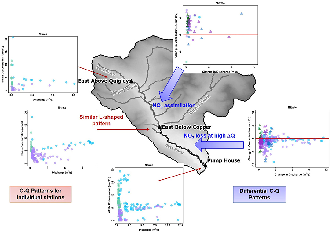
Figure 9. A comparison of C-Q hysteresis patterns for NO3 across individual stations and differential C-Q analyses across the upstream and downstream reaches encompassing those stations. The C-Q patterns show a consistent L-shaped pattern for NO3 across all three stations of the East River Catchment. In comparison, differential C-Q metrics show gains in nitrate in the upstream reach and losses in the downstream reach during high gains in discharge.
Data Availability Statement
Publicly available datasets were analyzed in this study. This data can be found here: http://dx.doi.org/10.21952/WTR/1495380.
Author Contributions
BA and CS designed the study. MB, MN, and DD were in charge of the technical aspects of this work. KW collected samples and provided ancillary data. RC provided discharge data and WD performed geochemical analyses. BA and MB wrote the manuscript, with edits from CS, RC, DD, WD, and SH. All authors contributed to the article and approved the submitted version.
Conflict of Interest
The authors declare that the research was conducted in the absence of any commercial or financial relationships that could be construed as a potential conflict of interest.
Acknowledgments
This material is based on work supported as part of the Aggregated Watershed Component of the Watershed Function Scientific Focus Area funded by the U.S. Department of Energy, Office of Science, Office of Biological and Environmental Research under Award no. DE-AC02-05CH11231.
Supplementary Material
The Supplementary Material for this article can be found online at: https://www.frontiersin.org/articles/10.3389/frwa.2020.00024/full#supplementary-material
References
Aich, V., Zimmermann, A., and Elsenbeer, H. (2014). Quantification and interpretation of suspended-sediment discharge hysteresis patterns: How much data do we need? Catena 122, 120–129. doi: 10.1016/j.catena.2014.06.020
Anderson, S. P., Dietrich, W. E., Torres, R., Montgomery, D. R., and Loague, K. (1997). Concentration-discharge relationships in runoff from a steep, unchanneled catchment. Water Resour. Res. 33, 211–225. doi: 10.1029/96WR02715
Arora, B., Dwivedi, D., Faybishenko, B., Jana, R. B., and Wainwright, H. M. (2019a). Understanding and predicting vadose zone processes. Rev. Mineral. Geochemistry 85, 303–328. doi: 10.2138/rmg.2019.85.10
Arora, B., Sengör, S. S., Spycher, N. F., and Steefel, C. I. (2015). A reactive transport benchmark on heavy metal cycling in lake sediments. Comput. Geosci. 19, 613–633. doi: 10.1007/s10596-014-9445-8
Arora, B., Spycher, N. F., Steefel, C. I., Molins, S., Bill, M., Conrad, M. E., et al. (2016). Influence of hydrological, biogeochemical and temperature transients on subsurface carbon fluxes in a flood plain environment. Biogeochemistry. 127, 367–396. doi: 10.1007/s10533-016-0186-8
Arora, B., Wainwright, H. M., Dwivedi, D., Vaughn, L. J., Curtis, J. B., Torn, M. S., et al. (2019b). Evaluating temporal controls on greenhouse gas (GHG) fluxes in an Arctic tundra environment: An entropy-based approach. Sci. Total Environ. 649, 284–299.
Battaglin, W. A., Hay, L. A., and Markstrom, S. L. (2012). Watershed Scale Response to Climate Change—East River. Basin: Colorado. doi: 10.3133/fs20113126
Bernal, S., Butturini, A., and Sabater, F. (2006). Inferring nitrate sources through end member mixing analysis in an intermittent Mediterranean stream. Biogeochemistry 81, 269–289. doi: 10.1007/s10533-006-9041-7
Bieroza, M. Z., Heathwaite, A. L., Bechmann, M., Kyllmar, K., and Jordan, P. (2018). The concentration-discharge slope as a tool for water quality management. Sci. Total Environ. 630, 738–749. doi: 10.1016/j.scitotenv.2018.02.256
Carroll, K. P., Rose, S., and Peters, N. E. (2007). Concentration/Discharge Hysteresis Analysis of Storm Events at the Panola Mountain Research. Watershed: Gerogia.
Carroll, R. W. H., Bearup, L. A., Brown, W., Dong, W., Bill, M., and Willlams, K. H. (2018). Factors controlling seasonal groundwater and solute flux from snow-dominated basins. Hydrol. Process. 32, 2187–2202. doi: 10.1002/hyp.13151
Carroll, R. W. H., Deems, J. S., Niswonger, R., Schumer, R., and Williams, K. H. (2019). The importance of interflow to groundwater recharge in a snowmelt-dominated headwater basin. Geophys. Res. Lett. 46, 5899–5908. doi: 10.1029/2019GL082447
Chanat, J. G., Rice, K. C., and Hornberger, G. M. (2002). Consistency of patterns in concentration-discharge plots. Water Resour. Res. 38, 22-1–22-10. doi: 10.1029/2001WR000971
Colorado Water Quality Control Commission (2012). Regulation No. 85. Nutrients Management Control Regulation. 5 CCR 1002-85.
Covino, T., McGlynn, B., and Mallard, J. (2011). Stream-groundwater exchange and hydrologic turnover at the network scale. Water Resour. Res. 47, 1–11. doi: 10.1029/2011WR010942
Deacon, J. R., and Driver, N. E. (1999). Distribution of trace elements in streambed sediment associated with mining activities in the upper colorado river basin, Colorado, USA, 1995–96. Arch. Environ. Contam. Toxicol. 37, 7–18. doi: 10.1007/s002449900484
Dong, W., Wan, J., Tokunaga, T. K., Gilbert, B., and Williams, K. H. (2017). Transport and humification of dissolved organic matter within a semi-arid floodplain. J. Environ. Sci. 57, 24–32. doi: 10.1016/j.jes.2016.12.011
Dwivedi, D., Arora, B., Steefel, C. I., Dafflon, B., and Versteeg, R. (2018a). Hot spots and hot moments of nitrogen in a riparian corridor. Water Resour. Res. 54, 205–222. doi: 10.1002/2017WR022346
Dwivedi, D., Steefel, C. I., Arora, B., Newcomer, M., Moulton, J. D., Dafflon, B., et al. (2018b). Geochemical exports to river from the intrameander hyporheic zone under transient hydrologic conditions: east river mountainous watershed, colorado. Water Resour. Res. 54, 8456–8477. doi: 10.1029/2018WR023377
Dwivedi, D., Steefel, I. C., Arora, B., and Bisht, G. (2017). Impact of intra-meander hyporheic flow on nitrogen cycling. Procedia Earth Planet. Sci. 17, 404–407. doi: 10.1016/j.proeps.2016.12.102
Evans, C., and Davies, T. D. (1998). Causes of concentration/discharge hysteresis and its potential as a tool for analysis of episode hydrochemistry. Water Resour. Res. 34, 129–137. doi: 10.1029/97WR01881
Gaskill, D. L., Mutschler, F. E., Kramer, J. H., Thomas, J. A., and Zahony, S. G. (1991). Geologic Map of the Gothic Quadrangle, Gunnison County, Colorado. Reston, VA: U.S. Geological Survey Map GQ-1969. U.S. Geological Survey.
Gellis, A. C. (2013). Factors influencing storm-generated suspended-sediment concentrations and loads in four basins of contrasting land use, humid-tropical Puerto Rico. Catena. 104, 39–57. doi: 10.1016/j.catena.2012.10.018
Godsey, S., Kirchner, J., and Clow, D. (2009). Concentration–discharge relationships reflect chemostatic characteristics of US catchments. Hydrol. Process. 23, 1844–1864. doi: 10.1002/hyp.7315
Gwenzi, W., Chinyama, S. R., and Togarepi, S. (2017). Concentration-discharge patterns in a small urban headwater stream in a seasonally dry water-limited tropical environment. J. Hydrol. 550, 12–25. doi: 10.1016/j.jhydrol.2017.04.029
Hall, F. R. (1970). Dissolved solids-discharge relationships: 1. Mixing Models. Water Resour. Res. 6, 845–850. doi: 10.1029/WR006i003p00845
Hamshaw, S. D., Dewoolkar, M. M., Schroth, A. W., Wemple, B. C., and Rizzo, D. M. (2018). A new machine-learning approach for classifying hysteresis in suspended-sediment discharge relationships using high-frequency monitoring data. Water Resour. Res. 54, 4040–4058. doi: 10.1029/2017WR022238
Hoagland, B., Russo, T. A., and Brantley, S. L. (2017). Relationships in a headwater sandstone stream. Water Resour. Res. 53, 4643–4667. doi: 10.1002/2016WR019717
Hornberger, G. M., Scanlon, T. M., and Raffensperger, J. P. (2001). Modelling transport of dissolved silica in a forested headwater catchment: the effect of hydrological and chemical time scales on hysteresis in the concentration-discharge relationship. Hydrol. Process. 15, 2029–2038. doi: 10.1002/hyp.254
Hubbard, S. S., Williams, K. H., Agarwal, D., Banfield, J., Beller, H., Bouskill, N., et al. (2018). The east river, colorado, watershed: a mountainous community testbed for improving predictive understanding of multiscale hydrological-biogeochemical dynamics. Vadose Zo. J. 17, 1–25. doi: 10.2136/vzj2018.03.0061
Junge, C. E., and Wurbe, R. T. (1958). The concentration of chloride, sodium, potassium and sulfate in rain water over the United States. J. Meteorol. 15, 417–425.
Kenwell, A., Navarre-Sitchler, A., Prugue, R., Spear, J. R., Hering, A. S., Maxwell, R. M., et al. (2016). Using geochemical indicators to distinguish high biogeochemical activity in floodplain soils and sediments. Sci. Total Environ. 563–564, 386–395. doi: 10.1016/j.scitotenv.2016.04.014
Knapp, J. L. A., von Freyberg, J., Studer, B., Kiewiet, L., and Kirchner, J. W. (2020). Concentration–discharge relationships vary among hydrological events, reflecting differences in event characteristics. Hydrol. Earth Syst. Sci. 24, 2561–2576. doi: 10.5194/hess-24-2561-2020
Koger, J. M., Newman, B. D., and Goering, T. J. (2018). Chemostatic behaviour of major ions and contaminants in a semiarid spring and stream system near Los Alamos, NM, USA. Hydrol. Process. 32, 1709–1716. doi: 10.1002/hyp.11624
Krause, S., Boano, F., Cuthbert, M. O., Fleckenstein, J. H., and Lewandowski, J. (2014). Understanding process dynamics at aquifer-surface water interfaces: an introduction to the special section on new modeling approaches and novel experimental technologies. Water Resour. Res. 50, 1847–1855. doi: 10.1002/2013WR014755
Lloyd, C. E. M., Freer, J. E., Johnes, P. J., and Collins, A. L. (2016). Using hysteresis analysis of high-resolution water quality monitoring data, including uncertainty, to infer controls on nutrient and sediment transfer in catchments. Sci. Total Environ. 543, 388–404. doi: 10.1016/j.scitotenv.2015.11.028
Markstrom, S. L., Hay, L. E., Ward-Garrison, C. D., Risley, J. C., Battaglin, W. A., Bjerklie, D. M., et al. (2012). Integrated Watershed-Scale Response to Climate Change for Selected Basins Across the United States. doi: 10.3133/sir20115077
McDonnell, J. J. (1990). A rationale for old water discharge through macropores in a steep, humid catchment. Water Resour. Res. 26, 2821–2832. doi: 10.1029/WR026i011p02821
McDonnell, J. J., Sivapalan, M., Vaché, K., Dunn, S., Grant, G., Haggerty, R., et al. (2007). Moving beyond heterogeneity and process complexity: a new vision for watershed hydrology. Water Resour. Res. 43, 1–6. doi: 10.1029/2006WR005467
Megnounif, A., Terfous, A., and Ouillon, S. (2013). A graphical method to study suspended sediment dynamics during flood events in the Wadi Sebdou, NW Algeria (1973–2004). J. Hydrol. 497, 24–36. doi: 10.1016/j.jhydrol.2013.05.029
Meybeck, M., and Moatar, F. (2012). Daily variability of river concentrations and fluxes: indicators based on the segmentation of the rating curve. Hydrol. Process. 26, 1188–1207. doi: 10.1002/hyp.8211
Milly, P. C. D., Betancourt, J., Falkenmark, M., Hirsch, R. M., Kundzewicz, Z. W., Lettenmaier, D. P., et al. (2008). Climate change. Stationarity is dead: whither water management? Science 319, 573–574. doi: 10.1126/science.1151915
Milne, A. E., Macleod, C. J. A., Haygarth, P. M., Hawkins, J. M. B., and Lark, R. M. (2009). The wavelet packet transform: a technique for investigating temporal variation of river water solutes. J. Hydrol. 379, 1–19. doi: 10.1016/j.jhydrol.2009.09.038
Moatar, F., Abbott, B. W., Minaudo, C., Curie, F., and Pinay, G. (2017). Elemental properties, hydrology, and biology interact to shape concentration-discharge curves for carbon, nutrients, sediment, and major ions. Water Resour. Res. 53, 1270–1287. doi: 10.1002/2016WR019635
Molins, S., Trebotich, D., Arora, B., Steefel, C. I., and Deng, H. (2019). Multi-scale model of reactive transport in fractured media: diffusion limitations on rates. Transport in Porous Media. 128, 701–721.
Morrison, S. J., Goodknight, C. S., Tigar, A. D., Bush, R. P., and Gil, A. (2012). Naturally occurring contamination in the mancos shale. Environ. Sci. Technol. 46, 1379–1387. doi: 10.1021/es203211z
Murphy, J. C., Hornberger, G. M., and Liddle, R. G. (2014). Concentration-discharge relationships in the coal mined region of the New River basin and Indian Fork sub-basin, Tennessee, USA. Hydrol. Process. 28, 718–728. doi: 10.1002/hyp.9603
Musolff, A., Schmidt, C., Selle, B., and Fleckenstein, J. H. (2015). Catchment controls on solute export. Adv. Water Resour. 86, 133–146. doi: 10.1016/j.advwatres.2015.09.026
Payn, R. A., Gooseff, M. N., McGlynn, B. L., Bencala, K. E., and Wondzell, S. M. (2009). Channel water balance and exchange with subsurface flow along a mountain headwater stream in Montana, United States. Water Resour. Res. 45, 1–14. doi: 10.1029/2008WR007644
Pearce, A. J., Stewart, M. K., and Sklash, M. G. (1986). Storm runoff generation in humid headwater catchments: 1. where does the water come from? Water Resour. Res. 22, 1263–1272. doi: 10.1029/WR022i008p01263
Pribulick, C. E., Foster, L. M., Bearup, L. A., Navarre-Sitchler, A. K., Williams, K. H., Carroll, R. W. H., et al. (2016). Contrasting the hydrologic response due to land cover and climate change in a mountain headwaters system. Ecohydrology 9, 1431–1438. doi: 10.1002/eco.1779
Rodríguez-Iturbe, I., Ijjász-Vásquez, E. J., Bras, R. L., and Tarboton, D. G. (1992). Power law distributions of discharge mass and energy in river basins. Water Resour. Res. 28, 1089–1093. doi: 10.1029/91WR03033
Rose, L. A., Karwan, D. L., and Godsey, S. E. (2018). Concentration-discharge relationships describe solute and sediment mobilization, reaction, and transport at event and longer timescales. Hydrol. Process. 32, 2829–2844. doi: 10.1002/hyp.13235
Rose, S. (2003). Comparative solute-discharge hysteresis analysis for an urbanized and a “control basin” in the Georgia (USA) Piedmont. J. Hydrol. 284, 45–56. doi: 10.1016/j.jhydrol.2003.07.001
Sklash, M. G., Stewart, M. K., and Pearce, A. J. (1986). Storm runoff generation in humid headwater catchments: 2. a case study of hillslope and low-order stream response. Water Resour. Res. 22, 1273–1282. doi: 10.1029/WR022i008p01273
Spahr, N. E. (2000). Water quality in the upper colorado river basin, colorado, 1996-98. U.S. Dep. Interior, U.S. Geol. Survey Circular. 1214. doi: 10.3133/cir1214
Sullivan, P. L., Stops, M. W., Macpherson, G. L., Li, L., Hirmas, D. R., and Dodds, W. K. (2018). How landscape heterogeneity governs stream water concentration-discharge behavior in carbonate terrains (Konza Prairie, USA). Chem. Geol. 527:118989. doi: 10.1016/j.chemgeo.2018.12.002
Szeftel, P., Moore, R. D., and Weiler, M. (2011). Influence of distributed flow losses and gains on the estimation of transient storage parameters from stream tracer experiments. J. Hydrol. 396, 277–291. doi: 10.1016/j.jhydrol.2010.11.018
Thompson, S. E., Basu, N. B., Lascurain, J., Aubeneau, A., and Rao, P. S. C. (2011). Relative dominance of hydrologic versus biogeochemical factors on solute export across impact gradients. Water Resour. Res. 47, 1–20. doi: 10.1029/2010WR009605
Tokunaga, T. K., Wan, J., Williams, K. H., Brown, W., Henderson, A., Kim, Y., et al. (2019). Depth- and time-resolved distributions of snowmelt-driven hillslope subsurface flow and transport and their contributions to surface waters. Water Resour. Res. 55, 9474–9499. doi: 10.1029/2019WR025093
Udall, B., and Overpeck, J. (2017). The twenty-first century Colorado River hot drought and implications for the future. Water Resour. Res. 53, 2404–2418. doi: 10.1002/2016WR019638
Wan, J., Tokunaga, T. K., Williams, K. H., Dong, W., Brown, W., Henderson, A. N., et al. (2019). Predicting sedimentary bedrock subsurface weathering fronts and weathering rates. Sci. Rep. 9:17198. doi: 10.1038/s41598-019-53205-2
Ward, A. S., Gooseff, M. N., Voltz, T. J., Fitzgerald, M., Singha, K., and Zarnetske, J. P. (2013). How does rapidly changing discharge during storm events affect transient storage and channel water balance in a headwater mountain stream? Water Resour. Res. 49, 5473–5486. doi: 10.1002/wrcr.20434
Williams, G. P. (1989). Sediment concentration versus water discharge during single hydrologic events in rivers. J. Hydrol. 111, 89–106. doi: 10.1016/0022-1694(89)90254-0
Williams, K. H., Long, P. E., Davis, J. A., Wilkins, M. J., N'Guessan, A. L., Steefel, C. I., et al. (2011). Acetate availability and its influence on sustainable bioremediation of uranium-contaminated groundwater. Geomicrobiol. J. 28, 519–539. doi: 10.1080/01490451.2010.520074
Winnick, M. J., Carroll, R. W. H., Williams, K. H., Maxwell, R. M., Dong, W., and Maher, K. (2017). Snowmelt controls on concentration-discharge relationships and the balance of oxidative and acid-base weathering fluxes in an alpine catchment, East River, Colorado. Water Resour. Res. 53, 2507–2523. doi: 10.1002/2016WR019724
Wood, P. A. (1977). Controls of variation in suspended sediment concentration in the River Rother, West Sussex, England. Sedimentology 24, 437–445. doi: 10.1111/j.1365-3091.1977.tb00131.x
Wymore, A. S., Brereton, R. L., Ibarra, D. E., Maher, K., and Mcdowell, W. H. (2017). Critical zone structure controls concentration-discharge relationships and solute generation in forested tropical montane watersheds. Water 53, 6279–6295. doi: 10.1002/2016WR020016
Keywords: streamflow, spatial variability, temporal variability, field observations, phosphorus, nitrate, concentration-discharge, shale mineralogy
Citation: Arora B, Burrus M, Newcomer M, Steefel CI, Carroll RWH, Dwivedi D, Dong W, Williams KH and Hubbard SS (2020) Differential C-Q Analysis: A New Approach to Inferring Lateral Transport and Hydrologic Transients Within Multiple Reaches of a Mountainous Headwater Catchment. Front. Water 2:24. doi: 10.3389/frwa.2020.00024
Received: 30 March 2020; Accepted: 14 July 2020;
Published: 19 August 2020.
Edited by:
Michael Bliss Singer, Cardiff University, United KingdomReviewed by:
Scott W. Bailey, United States Forest Service (USDA), United StatesLucy Rose, University of Minnesota Twin Cities, United States
Copyright © 2020 Arora, Burrus, Newcomer, Steefel, Carroll, Dwivedi, Dong, Williams and Hubbard. This is an open-access article distributed under the terms of the Creative Commons Attribution License (CC BY). The use, distribution or reproduction in other forums is permitted, provided the original author(s) and the copyright owner(s) are credited and that the original publication in this journal is cited, in accordance with accepted academic practice. No use, distribution or reproduction is permitted which does not comply with these terms.
*Correspondence: Bhavna Arora, YmFyb3JhQGxibC5nb3Y=