Parametrization of Stochastic Inputs Using Generative Adversarial Networks With Application in Geology

We investigate artificial neural networks as a parametrization tool for stochastic inputs in numerical simulations. We address parametrization from the point of view of emulating the data generating process, instead of explicitly constructing a parametric form to preserve predefined statistics of the data. This is done by training a neural network to generate samples from the data distribution using a recent deep learning technique called generative adversarial networks. By emulating the data generating process, the relevant statistics of the data are replicated. The method is assessed in subsurface flow problems, where effective parametrization of underground properties such as permeability is important due to the high dimensionality and presence of high spatial correlations. We experiment with realizations of binary channelized subsurface permeability and perform uncertainty quantification and parameter estimation. Results show that the parametrization using generative adversarial networks is very effective in preserving visual realism as well as high order statistics of the flow responses, while achieving a dimensionality reduction of two orders of magnitude.

1. Introduction

Many problem scenarios such as uncertainty quantification and parameter estimation involve the solution of partial differential equations with a stochastic input. This is because in many real applications, some properties of the system are uncertain or simply unknown. The general approach is to use a probabilistic framework where we represent such uncertainties as random variables with a predefined distribution. In some cases where both the distribution and the forward map are trivial, a closed-form solution is possible; however this is very rarely the case. Often in practice, we can only resort to a brute-force approach where we draw several realizations of the random variables, e.g., using Markov chain Monte Carlo sampling, and fully solve the partial differential equations for each realization in an effort to estimate distributions or bounds of the system's response. This approach suffers from slow convergence and the need to perform a large number of forward simulations, which led to the development of several methods to reduce the computational burden of this task.

A straightforward solution is to reduce the computational cost of the forward map itself—numerous methods exist in this direction, including reduced-order models (Lassila et al., 2014; Jin et al., 2019; Kani and Elsheikh, 2019), surrogate models (Razavi et al., 2012; Qin et al., 2019; Tarakanov and Elsheikh, 2019), and upscaling (Christie and Blunt, 2001; Chan and Elsheikh, 2018a; Vasilyeva and Tyrylgin, 2018). Another different direction consists of reducing or refining the search space or distribution of the random variables, for example by regularization or parametrization, thus reducing the number of simulations required. Parametrization is specially useful in problems where the number of random variables is huge but the variables are highly redundant and correlated. This is generally the case in subsurface flow problems: Complete prior knowledge of subsurface properties (e.g., porosity or permeability) is impossible, yet is very influential in the flow responses. At the same time, accurate flow modeling often requires the use of extremely large simulation grids. When the subsurface property is discretized, the number of free variables is naively associated with the number of grid cells. The random variables thus obtained are hardly independent, whose assumption during the modeling leads to unnecessary computations. The goal of parametrization is to discover statistical relationships between the random variables in order to obtain a reduced and more effective representation.

The importance of parametrization in subsurface simulations resulted in a variety of methods in the literature including zonation (Jacquard, 1965; Jahns, 1966) and zonation-based methods (Bissell, 1994; Chavent and Bissell, 1998; Grimstad et al., 2001, 2002, 2003; Aanonsen, 2005), PCA-based methods (Gavalas et al., 1976; Oliver et al., 1996; Reynolds et al., 1996; Sarma et al., 2008; Ma and Zabaras, 2011; Vo and Durlofsky, 2016), SVD-based methods (Tavakoli and Reynolds, 2009, 2011; Shirangi, 2014; Shirangi and Emerick, 2016), discrete wavelet transform (Mallat, 1989; Lu and Horne, 2000; Sahni and Horne, 2005), discrete cosine transform (Jafarpour and McLaughlin, 2007, 2009; Jafarpour et al., 2010), level set methods (Moreno and Aanonsen, 2007; Dorn and Villegas, 2008; Chang et al., 2010), and dictionary learning (Khaninezhad et al., 2012a,b). Many methods begin by proposing parametric forms for the random vector to be modeled which are then explicitly fitted to preserve certain chosen statistics. In the process, many methods inevitably adopt some simplifying assumptions, either on the parametric form to be employed or the statistics to be reproduced, which are necessary for the method to be actually feasible. In this work, we consider the use of neural networks for both parametrization of the random vector and definition of its relevant statistics. This is motivated by recent advances in the field of machine learning (Goodfellow et al., 2014; Radford et al., 2015; Arjovsky et al., 2017) and the high expressive power of neural networks (Hornik et al., 1989) that makes them one of the most flexible forms of parametrization.

The idea is to obtain a parametrization by emulating the data generating process. We seek to construct a function called the generator—in this case, a neural network—that takes a low-dimensional vector as input (the reduced representation), and aims to output a realization of the target random vector. The low-dimensional vector is assumed to come from an easy-to-sample distribution, e.g., a multivariate normal or an uniform distribution, and is what provides the element of stochasticity. Generating a new realization then only requires sampling the low-dimensional vector and a forward pass of the generator network. The neural network is trained using a dataset of prior realizations that inform the patterns and variability of the random vector (e.g., geological realizations from a database or from multipoint geostatistical simulations; Strebelle and Journel, 2001; Mariethoz and Caers, 2014).

The missing component in the description above is the definition of an objective function to actually train such generator; in particular, how do we quantify the discrepancy between generated samples and actual samples? This is resolved using a recent technique in machine learning called generative adversarial networks (Goodfellow et al., 2014) (GAN). The idea in GAN is to let a second classifier neural network, called the discriminator, define the objective function. The discriminator takes the role of an adversary against the generator where both are trained alternately in a minmax game: the discriminator is trained to maximize a classification performance where it needs to distinguish between “fake” (from the generator) and “real” (from the dataset) samples, while the generator is trained to minimize it. Hence, the generator is iteratively trained to generate good realizations in order to fool the discriminator, while the discriminator is in turn iteratively trained to improve its ability to classify correctly. In the equilibrium of the game, the generator effectively learns to generate plausible samples, and the discriminator regards all samples as equally plausible (coin toss scenario).

The benefit of this approach is that we do not need to manually specify which statistics of the data need to be preserved, instead we let the discriminator network implicitly learn the relevant statistics. We can see that the high expressive power of neural networks is leveraged in two aspects: on one hand, the expressive power of neural networks allows the effective parametrization (generator) of complex realizations; on the other hand, it allows the discriminator to learn the complex statistics of the data.

This work is an extension of our preliminary work in Chan and Elsheikh (2017). There is a growing number of recent works in geology where GANs have been studied, including porous media reconstruction (Mosser et al., 2017a,b), seismic inversion (Mosser et al., 2018a), parameter estimation (Laloy et al., 2018; Canchumuni et al., 2019; Mosser et al., 2019; Zhang et al., 2019), conditional geological models (Chan and Elsheikh, 2018b; Dupont et al., 2018; Mosser et al., 2018b), subsurface plume modeling (Zhong et al., 2019), carbon storage Graham and Chen (2020), and 2D-to-3D geological modeling (Coiffier and Renard, 2019). Other methods similar to GAN include (Laloy et al., 2017; Liu and Durlofsky, 2019; Liu et al., 2019) where a neural network parametrization of the subsurface is obtained. Currently, there is increasing interest in applying machine learning techniques to address geological problems (Bergen et al., 2019; Sun and Scanlon, 2019)

In this work, we provide further assessments and focus mainly on the capabilities of GAN as a parametrization tool to preserve high order flow statistics and visual realism. We parametrize binary channelized permeability models based on the classical Strebelle training image (Strebelle and Journel, 2001), a benchmark problem that is often employed for assessing parametrization methods due to the difficulties in crisply preserving the channels. To assess the method, we consider uncertainty propagation in subsurface flow problems for a large number of realizations of the permeability and compare the statistics in their flow responses. We also perform parameter estimation using natural evolution strategies (Wierstra et al., 2008, 2014), a general black-box optimization method that is suitable for the obtained reduced representation. Finally, we discuss training difficulties of GAN encountered during our implementation—in particular, limitations in small datasets, and inherent issues of the standard formulation of GAN (Goodfellow et al., 2014).

The rest of this chapter is organized as follows: In section 2, we briefly describe convolutional neural networks—a widely used architecture in modern neural networks—and the method of generative adversarial networks. Section 3 contains our numerical results for uncertainty quantification and parameter estimation experiments. In section 4, we provide a discussion for practical implementation. We draw our conclusions in section 5.

2. Background

2.1. Convolutional Neural Networks

A (feedforward) neural network is a composition of functions f(x) = f^L(f^L−1(⋯(f¹(x)))) where each function f^l(x), called a layer, is of the form σ_l(W_lx + b_l), i.e., an affine transform followed by a component-wise non-linearity. The choice of the number of layers L, the non-linear functions σ_l, and the sizes of W_l, b_l are part of the architecture design process, which is largely problem-dependent and based on heuristics and domain knowledge. Modern architectures use non-linearities such as rectifier linear units (ReLU, σ(x) = x⁺ = max(0,x)), leaky rectifier linear units (leaky ReLU, σ(x) = x⁺+0.01x⁻), tanh, sigmoid, and others; and can have as much as 100 layers (Simonyan and Zisserman, 2014; He et al., 2016). After an architecture is assumed, the weights of W_l, b_l are obtained by optimization of an objective.

A major architectural choice that led to huge advances in computer vision is the use of convolutional layers (Fukushima and Miyake, 1982). An example of a convolution is the following: Let u = (u₁, ⋯, u_m) be an input vector and k = (w₁, w₂) be a filter. The output of convolving the filter k on u is v = (v₁, ⋯, v_p) where v_i = w₁u_i + w₂u_{i + 1} (using stride 1). The operation is illustrated in Figure 1 : In a traditional fully connected layer, the associated matrix is dense and all its weights need to be determined in optimization. In a convolutional layer, the connections are constrained in such a way that each output component only depends on a neighborhood of the input, and as a result the associated matrix is a sparse diagonal-constant matrix, thus obtaining a huge reduction in the number of free weights. Note that in practice several stacks of convolution layers are used, so the full connectivity can be recovered if necessary. On top of the reduction, another benefit comes from the inherent regularization that this operator imposes that is often useful in applications where there is a spatial or temporal extent and the assumption of data locality is valid—informally, closer events in the spatial/temporal extent tend to be correlated (e.g., in natural images and speech).

FIGURE 1

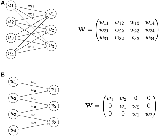
Figure 1. Transformation matrix of a fully connected layer (A), and of a convolutional layer (B). In this example, the convolutional layer has only 2 free weights, whereas the fully connected layer has 12 free weights.

The convolution as described above has a downscaling effect, i.e., the output size is always smaller or equal to the input size, which can be controlled by the filter stride. A classifier neural network typically consists of a series of convolutional layers that successively downscale an image to a single number (binary classification) or a vector of numbers (multiclass classification). In the case of decoders and generative networks, we wish to achieve the opposite effect to get an output that is larger than the input (e.g., to reconstruct an image from a compressed code). This can be achieved by simply transposing the convolutions: Using the example in Figure 1B, to convert from v to u, we can consider weight matrices of the form W^⊤, i.e., the transpose of the convolution matrix from u to v. Modern decoders and generators consist of a series of transposed convolutions that successively upscale a small vector to a large output array, e.g., corresponding to an image or audio.

The operations and properties discussed so far extend naturally to 2D and 3D arrays. For a 2D or 3D input array, the filter is also a 2D or 3D array, respectively. Note however that in the 3D case, the filter array is such that the depth (perpendicular to the spatial extent) is always equal to the depth of the 3D input array, therefore the output is always a 2D array, and the striding is done in the spatial extent (width and height). On the other hand, we allow the application of multiple filters to the same input, thereby producing a 3D output array if required, consisting of the stack of multiple convolution outputs. This way of operating with convolutions is inherited from image processing: Color images are 3D arrays consisting of three 2D arrays indicating the red, green, and blue intensities (in RGB format). Image filtering normally operates on all three values, e.g., the grayscale filter is v_ij = 0.299·u_{ij, red} + 0.587·u_{ij, green} + 0.114·u_{ij, blue}. The output of a convolution filter is also called a feature map.

Finally, we show in Figure 2 a popular pyramid architecture used in generator networks (Radford et al., 2015) for image synthesis. The blocks shown represent the state shapes (stack of feature maps) as the input vector is passed through the network. The input vector z is first treated as a “1-pixel image” (with many “feature maps”). The blocks are subsequently expanded in the spatial extent (width and height) while thinned in depth: A series of transposed convolutions is used to upsample the spatial extent until reaching the desired size; at the same time, the number of convolution filters is initially large, but it is subsequently reduced in the following layers. For classifier networks, usually the inverted architecture is used where the transposed convolutions are replaced with normal convolutions. Further notes on modern convolutional neural networks can be found in Karpathy (2020).

FIGURE 2

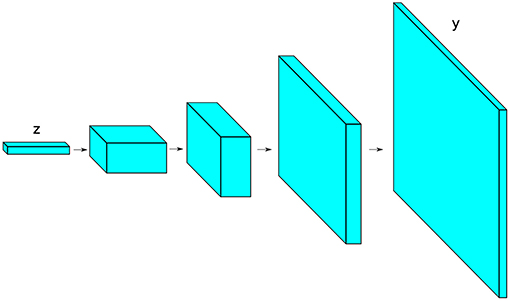
Figure 2. Illustration of a typical pyramid architecture used in generator networks.

2.2. Generative Adversarial Networks

Let z ~ p_z, y ~ ℙ_y, where p_z is a known, easy-to-sample distribution (e.g., multivariate normal or uniform distribution), and ℙ_y is the unknown distribution of interest (e.g., the distribution of all possible geomodels in a particular zone). The distribution ℙ_y is only known through realizations {y₁, y₂, ⋯, y_n} (e.g., realizations provided by multipoint geostatistical simulations). Let $G_{\theta }:{Z}\to {Y}$ be a neural network—called the generator—parametrized by weights θ to be determined. Given p_z fixed, this neural network induces a distribution G_θ(z) ~ ℙ_θ that depends on θ, and whose explicit form is complicated or intractable (since neural networks contain multiple non-linearities). On the other hand, sampling from this distribution is easy since it only involves sampling z and a forward evaluation of G_θ. The goal is to find θ such that ℙ_θ = ℙ_y.

Generative adversarial networks (GAN) (Goodfellow et al., 2014) approach this problem by considering a second classifier neural network—called the discriminator—to classify between “fake” samples (generated by the generator) and “real” samples (coming from the dataset of realizations). Let $D_{\psi }:{Y}\to \left[0,1\right]$ be the discriminator network parametrized by weights ψ to be determined. The training of the generator and discriminator uses the following loss function:

$\begin{array}{ll}L(\psi ,\theta ):={\displaystyle \underset{\text{y}~{\mathbb{P}}_y}{𝔼}}log{D}_{\psi }(\text{y})+{\displaystyle \underset{\tilde{\text{y}}~{\mathbb{P}}_{\theta }}{𝔼}}log(1-D_{\psi }(\tilde{\text{y}}))& (1)\end{array}$

where $\tilde{\text{y}}=G_{\theta }(\text{z})~{\mathbb{P}}_{\theta }$. In effect, this loss is the classification score of the discriminator, therefore we train D_ψ to maximize this function, and G_θ to minimize it:

$\begin{array}{ll}{\displaystyle \underset{\theta }{min}}{\displaystyle \underset{\psi }{max}}L(\psi ,\theta )& (2)\end{array}$

In practice, optimization of this minmax game is done alternately using some variant of stochastic gradient descent, where the gradient can be obtained using automatic differentiation algorithms. In the infinite capacity setting, this optimization amounts to minimizing the Jensen-Shannon divergence between ℙ_y and ℙ_θ (Goodfellow et al., 2014). Equilibrium of the game occurs when ℙ_y = ℙ_θ and $D_{\psi }=\frac{1}{2}$ in the support of ℙ_y (coin toss scenario).

2.2.1. Wasserstein GAN

In practice, optimization of the minmax game (2) is known to be very unstable, prompting numerous works to understand and address this issue (Radford et al., 2015; Salimans et al., 2016; Arjovsky and Bottou, 2017; Arjovsky et al., 2017; Berthelot et al., 2017; Gulrajani et al., 2017; Kodali et al., 2017; Qi, 2017). One recent advance is to use the Wasserstein formulation of GAN (WGAN) (Arjovsky et al., 2017; Gulrajani et al., 2017). This formulation proposes the objective function

$\begin{array}{ll}L(\psi ,\theta ):={\displaystyle \underset{\text{y}~{\mathbb{P}}_y}{𝔼}}{D}_{\psi }(\text{y})-{\displaystyle \underset{\tilde{\text{y}}~{\mathbb{P}}_{\theta }}{𝔼}}{D}_{\psi }(\tilde{\text{y}})& (3)\end{array}$

and a constraint in the search space of D_ψ,

$\begin{array}{ll}{\displaystyle \underset{\theta }{min}}{\displaystyle \underset{\psi :D_{\psi }\in D}{max}}L(\psi ,\theta )& (4)\end{array}$

where now $D_{\psi }:{Y}\to ℝ$ and ${D}$ is the set of 1-Lipschitz functions. This constraint can be loosely enforced by constraining the weights ψ to a compact space, e.g., by clipping the values of the weights in an interval [−c, c]. In this case, ${D}$ is a set of k-Lipschitz functions where the constant k depends on c and is irrelevant for optimization. Other approaches to enforce the constraint include penalizing the gradients of D (Gulrajani et al., 2017; Mroueh et al., 2017) and normalizing the weights of D (Miyato et al., 2018).

Although the modifications in Equations (3) and (4) over Equations (1) and (2) seem trivial, the derivation of this formulation is rather involved and can be found in Arjovsky et al. (2017). In essence, this formulation aims to minimize the Wasserstein distance between two distributions, instead of the Jensen-Shannon divergence. Here we only highlight important consequences of this formulation:

• Available meaningful loss metric. This is because

$\begin{array}{ll}W({\mathbb{P}}_y,{\mathbb{P}}_{\theta })\approx {\displaystyle \underset{\psi :D_{\psi }\in D}{max}}L(\psi ,\theta )& (5)\end{array}$

where W denotes the Wasserstein distance.

• Better stability. In particular, mode collapse is drastically reduced (see section 4.1).

• Robustness to architectural choices and optimization parameters.

We experimentally verify these points in section 4.1 and discuss their implications for our current application.

A pseudo-code of the training process is shown in Algorithm 1. Note that D is trained multiple times (n_D) per each iteration of G. This is to keep D near optimality so that the Wasserstein estimate in Equation (5) is accurate before every update of G. We also note that even though we show a simple gradient ascent/descent in the update steps (lines 6 and 11), it is more common to use update schemes such as RMSProp (Tieleman and Hinton, 2012) and Adam (Kingma and Ba, 2014) that are better suited for neural network optimization.

ALGORITHM 1

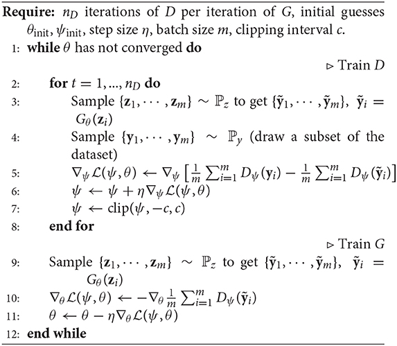
Algorithm 1: The WGAN algorithm

3. Numerical Experiments

We perform parametrization of unconditional and conditional realizations (point conditioning) of size 64 × 64 of a binary channelized permeability by training GAN using 1,000 prior realizations. The training image is the benchmark image by Strebelle (Strebelle and Journel, 2001) containing meandering left-to-right channels. The conditioning is done at 16 locations, summarized in Table 1, containing 13 locations of high permeability (channel material) and 3 locations of low permeability (background material). The channel has a log-permeability of 1 and the background has a log-permeability of 0, however for the purpose of training GAN we shall use −1 to denote the background, and restore the value to 0 for the flow simulations. The prior realizations are generated using the SNESIM algorithm (Strebelle and Journel, 2001). Examples of such realizations are shown in the top rows of Figures 3, 4.

TABLE 1

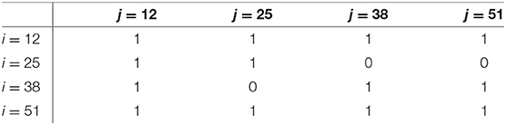
Table 1. Point conditioning at 16 locations, indicated by cell indices (i, j), regularly distributed across the domain.

FIGURE 3

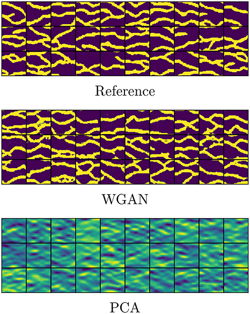
Figure 3. Unconditional realizations.

FIGURE 4

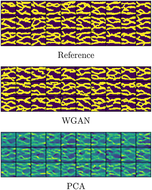
Figure 4. Conditional realizations.

3.1. Implementation

We train separate WGAN models for unconditional and conditional realizations. The architecture is the pyramid structure as described in section 2.1 and shown in Figure 2: For the generator, the input array is initially upscaled to size 4 × 4 in the spatial extent, and the initial number of feature maps is 512. This “block” is successively upscaled in the spatial extent and reduced in the number of feature maps both by a factor of 2, until the spatial extent reaches size 32 × 32. A final transposed convolution upscales the block to the output size of 64 × 64. The non-linearities are ReLUs for all layers except the last layer where we use tanh(·) (so that the output is bounded in [−1, 1]—as noted above, we denote the background with −1 and the channels with 1). The discriminator architecture is a mirror version of the generator architecture, where the initial number of feature maps is 8. The block is successively downscaled in the spatial extent and increased in the number of feature maps by a factor of 2, until the spatial extent reaches size 4 × 4. A final convolutional filter reduces this block to a single real value. Note that the size of the discriminator (in terms of total number of weights) is 1/8 times smaller than the generator, which is justified below in section 4.2. All layers except the last use leaky ReLUs. The last layer does not use a non-linearity. We use $\text{z}~{N}(0,\text{I})$ of dimension 30. This was chosen using principal component analysis as a rule of thumb: to retain 75% of the energy, 54 and 94 eigencomponents are required in the unconditional and conditional cases, respectively. We chose a smaller number to further challenge the parametrization. The result is a dimensionality reduction of two orders of magnitude, from 4, 096 = 64 × 64 to 30.

The network is trained using a popular gradient update scheme called Adam, with β₁ = 0.5, β₂ = 0.999 (see Kingma and Ba, 2014). We use a step size of 10⁻⁴, batch size of 32, and clipping interval [−0.01, 0.01]. We perform 5 discriminator iterations per generator iteration. In our experiments, convergence was achieved in around 20,000 generator iterations. The total training time was around 30 min using an Nvidia GeForce GTX Titan X GPU. During deployment, the model can generate realizations of 64 × 64 size at the rate of about 5,500 realizations per second.

In Figures 3, 4 we show unconditional and conditional realizations generated by our trained models, and realizations generated by SNESIM (reference). We also show realizations generated with principal component analysis (PCA), retaining 75% of the energy. We see that our model clearly reproduces the visual patterns present in the prior realizations. In Figure 5 we show histograms of the permeability at 10 randomly selected locations, based on sets of 5000 fresh realizations generated by SNESIM (i.e., not from the prior set) and by WGAN. We find that our model generates values that are very close to either 0 or 1, and almost no value in between (no thresholding has been performed at this stage, only shifting and scaling to move the tanh interval [−1, 1] to [0, 1], i.e., (x + 1)/2). The histograms are remarkably close.

FIGURE 5

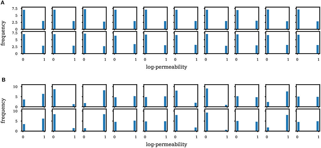
Figure 5. Histogram of permeability at 10 random locations based on SNESIM (first row) and WGAN (second row) realizations. (A) Unconditional case. (B) Conditional case.

3.2. Assessment in Uncertainty Quantification

In this section, we perform uncertainty quantification and estimate several flow statistics of interest. We borrow test cases from Ma and Zabaras (2011), where the authors parametrize the same type of permeability using Kernel PCA. Thus, we refer the interested reader to such work for results using Kernel PCA. Note that here we use a larger grid (64 × 64 vs. 45 × 45) and provide an additional flow test case.

We propagate 5,000 realizations of the permeability field in 2D single-phase subsurface flow. We consider injection of water for the purpose of displacing oil inside a reservoir (water and oil in this case have the same fluid properties since we consider single-phase flow). The system of equations for this problem is

$\begin{array}{lll}-\nabla ·(a\nabla p)& =q& (6)\end{array}$

$\begin{array}{lll}\phi \frac{\partial s}{\partial t}+\nabla ·(sv)& =q_w& (7)\end{array}$

where p is the fluid pressure, q = q_w + q_o denotes (total) fluid sources, q_w and q_o are the water and oil sources, respectively, a is the permeability, φ is the porosity, s is the saturation of water, and v is the Darcy velocity.

Our simulation domain is the unit square with 64 × 64 discretization grid. The reservoir initially contains only oil, i.e., s(x, t = 0) = 0, and we simulate from t = 0 until t = 0.4. We assume an uniform porosity of φ = 0.2. We consider two test cases:

Uniform flow: We impose uniformly distributed inflow and outflow conditions on the left and right sides of the unit square, respectively, and no-flow boundary conditions on the remaining top and bottom sides. The total absolute injection/production rate is 1. For the unit square, this means $v·\widehat{n}=-1$ and $v·\widehat{n}=1$ on the left and right sides, respectively, where $\widehat{n}$ denotes the outward-pointing unit normal to the boundary.

Quarter-five spot: We impose injection and production points at (0, 0) and (1, 1) of the unit square, respectively. No-flow boundary conditions are imposed on all sides of the square. The absolute injection/production rate is 1, i.e., q(0, 0) = 1 and q(1, 1) = −1.

The propagation is done on sets of realizations generated by WGAN and by SNESIM for comparison. Note that these are fresh realizations not used to train the WGAN models. We also show results using PCA for additional comparison.

Statistics of the saturation map based on 5,000 realizations are summarized in Figures 6, 7. We plot the saturation at time t = 0.1, which corresponds to 0.5 pore volume injected (PVI). From left to right, we plot the mean, variance, skewness and kurtosis of the saturation map. We see that the statistics from realizations generated by WGAN correspond very well with the statistics from realizations generated by SNESIM (reference). We also see that the PCA parametrization performs very well in the mean and variance, however the discrepancies increase as we move to higher order moments. The discrepancy becomes clearer by plotting the histogram of the 5,000 saturations at a fixed point in the domain, shown on the last columns of Figures 6, 7. We choose the point in the domain where reference saturation had the highest variance. We see that the histograms by WGAN match the reference remarkably well even in multimodal cases. The reader may compare our results with Ma and Zabaras (2011). The results suggest that the generator effectively learned to replicate the data generating process.

FIGURE 6

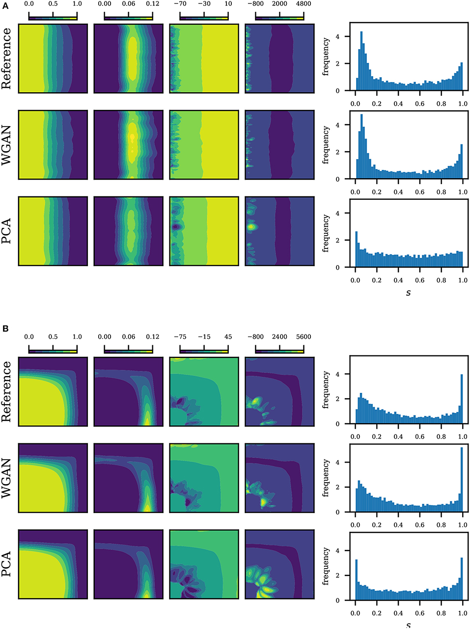
Figure 6. Saturation statistics at t = 0.5 PVI for unconditional realizations. From left to right: mean, variance, skewness and kurtosis of the saturation map, and lastly the saturation histogram at a given point. The point corresponds to the maximum variance in the reference. (A) Uniform flow, unconditional realizations. (B) Quarter five, unconditional realizations.

FIGURE 7

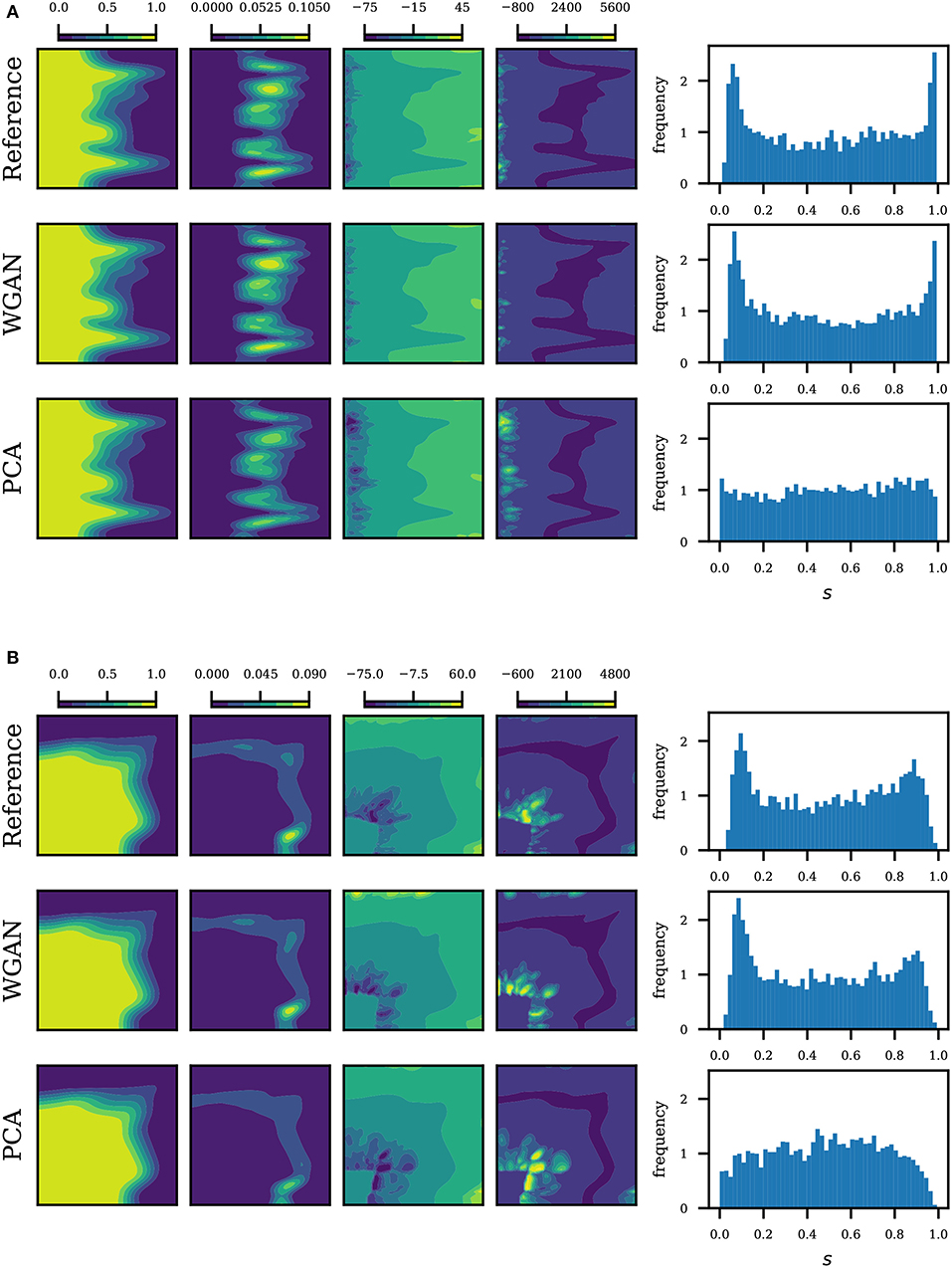
Figure 7. Saturation statistics at t = 0.5 PVI for conditional realizations. From left to right: mean, variance, skewness and kurtosis of the saturation map, and lastly the saturation histogram at a given point. The point corresponds to the maximum variance in the reference. (A) Uniform flow, conditional realizations. (B) Quarter five, conditional realizations.

Statistics of the production curve are summarized in Figures 8, 9. On the top half of each subfigure, we show the mean and variance of the production curve based on 5,000 realizations. These can in general be approximated well enough by using only the PCA parametrization. We find that the performance of our models are also comparable for this task. To further contrast the ability to preserve higher order statistics, we plot the histogram of the water breakthrough time, for which an accurate estimation is of importance in practice. Here we define the water breakthrough time as the time that water level reaches 1% of production. Results are shown on the bottom half of each subfigure in Figures 8, 9. In all cases, we find a very good agreement between WGAN and reference. Unlike PCA, the responses predicted by WGAN do not have a tendency to be normally distributed (see e.g., Figure 9A).

FIGURE 8

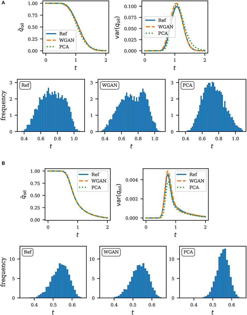
Figure 8. Production statistics for unconditional realizations. The top of each subfigure shows the mean and variance of the production curve. The bottom shows the histogram of the water breakthrough time. Times are expressed in pore volume injected. (A) Uniform flow, unconditional realizations. (B) Quarter five, unconditional realizations.

FIGURE 9

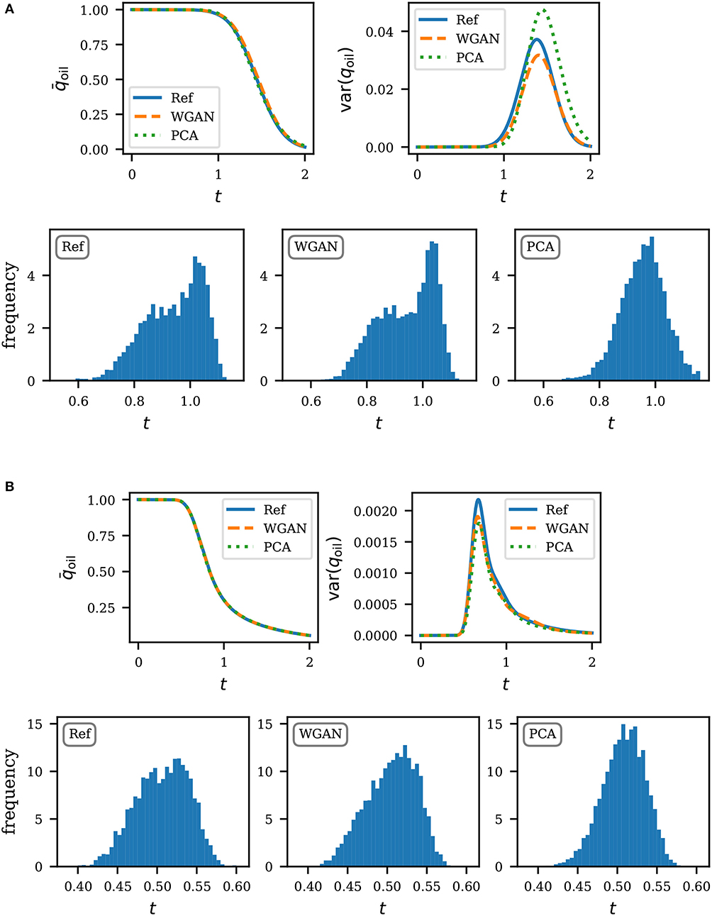
Figure 9. Production statistics for conditional realizations. The top half of each subfigure shows the mean and variance of the production curve. The bottom show the histogram of the water breakthrough time. Times are expressed in pore volume injected. (A) Uniform flow, conditional realizations. (B) Quarter five, conditional realizations.

3.3. Assessment in Parameter Estimation

We now assess our models for parameter estimation where we reconstruct the subsurface permeability based on historical data of the oil production stage, also known as history matching. Following the general problem setting from before, we aim to find realizations of the permeability that match the production curves observed from wells.

3.3.1. Inversion Using Natural Evolution Strategies

Let $\text{d}={M}(\text{a})$ where ${M}$ is the forward map, mapping from permeability a to the output d being monitored (in our case, the water level curve at the production wells). Given observations d_obs and assuming i.i.d. Gaussian measurement noise (we use σ = 0.01), and prior $\text{z}~{N}(0,\text{I})$, the objective function to be maximized is

$\begin{array}{lll}f(\text{z})& =-\frac{1}{{\sigma }^2}{(\text{d}-{\text{d}}_{\text{obs}})}^T(\text{d}-{\text{d}}_{\text{obs}})-{\text{z}}^T\text{z}& (8)\end{array}$

$\begin{array}{ll}=-\frac{1}{{\sigma }^2}{({M}(G(z))-d_{\text{obs}})}^T({M}(G(z))-d_{\text{obs}})-z^{T}z& (9)\end{array}$

To maximize this function, we use natural evolution strategies (NES) (Wierstra et al., 2008, 2014), a black-box optimization method suitable for the low-dimensional parametrization achieved. Another reasonable alternative is to use gradient-based methods exploiting the differentiability of our generator, as investigated in Laloy et al. (2019). This would require adjoint procedures to get the gradient of the forward map ${M}$. We adopted NES due to its generality and easy implementation that does not involve the gradient of f (nor ${M}$). NES maximizes f by maximizing an average of f instead, J(ϕ): = 𝔼_π(z|ϕ)f(z), where π(z|ϕ) is some distribution parametrized by ϕ (e.g., we used the family of Gaussian distributions, in which case ϕ involves the mean and covariance matrix). This is based on the observation that $\underset{\varphi }{max}{𝔼}_{\pi (\text{z}|\varphi )}f(\text{z})\le \underset{\text{z}}{max}f(\text{z})$.

Optimizing the expectation 𝔼_π(z|ϕ)f(z) (instead of optimizing f directly) has the advantage of not requiring the gradient of f (and therefore of the simulator) since

${\nabla }_{\varphi }J(\varphi )={𝔼}_{\pi (\text{z}|\varphi )}f(\text{z}){\nabla }_{\varphi }log\pi (\text{z}|\varphi )$

We can approximate this as

${\nabla }_{\varphi }J(\varphi )\approx \frac{1}{N}{\displaystyle \sum _{k=1}^N}f({\text{z}}_k){\nabla }_{\varphi }log\pi ({\text{z}}_k|\varphi )$

by drawing realizations z₁, ⋯, z_N ~ π(z|ϕ). Optimization proceeds by simple gradient ascent, ϕ ← ϕ + η∇_ϕJ(ϕ) where η is a step size. Note that we optimize the parameter of the search distribution ϕ, rather than z. As the optimization converges, the search distribution collapses to an optimal value of z. In our implementation, we actually use an improved version of NES which uses the Fisher matrix and natural coordinates, as detailed in Wierstra et al. (2014).

3.3.2. History Matching

We consider five target images of the permeability: one unconditional realization and one conditional realization (both using SNESIM), and three hand-crafted images (see first column in Figure 11). The latter were specifically designed to test the limits of the parametrization. For the conditional realization, we use the generator trained on conditional realizations. For the remaining cases, we use the unconditional generator. Note that this poses a difficulty on the reconstruction of the hand-crafted toy problems as these are not plausible realizations with respect to the dataset used to train the generator.

In each test case, we set one injection well with fixed flow rate of 1, and five production wells with flow rate of −0.2 (locations marked on each image, see Figure 11). Our only observed data are the water level curves at the production wells from t = 0 to t = 0.5PVI, induced by the target permeabilities. We do not include knowledge of the permeability at the “drilled” wells (as normally done in real applications) in the parameter estimation. For the experiments, we scaled the log-permeability values of 0 and 1 to 0 and 5, emulating a shale and sand scenario. We have done this in part to allow for a less underdetermined system (i.e., so that different permeability patterns produce more distinctive flow patterns).

Results for history matching are shown in Figures 10, 11. For each test case, we find three solutions of the inversion problem using different seeds (initial guess). For the conditional and unconditional realizations, we obtain virtually perfect match of the observed period (Figure 10). Beyond the observed period, the responses naturally diverge. As is expected, the matching is more difficult for some of the toy problems, in particular toy problem E and toy problem Z. Toy problem X, however, does particularly well.

FIGURE 10

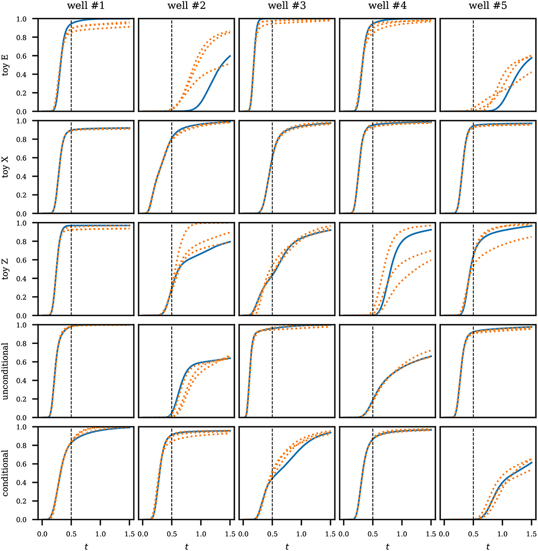
Figure 10. History matching results. Water level curves from the production wells in different test cases. Blue solid lines denote the target responses. Orange dotted lines are three matching solutions found in the inversion. The black vertical dashed line in each plot marks the end of the observed period. Times are expressed in pore volume injected.

FIGURE 11

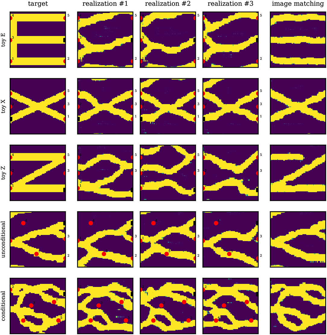
Figure 11. History matching results. We experiment with three toy images as well as unconditional and conditional SNESIM realizations. Each case contains one injection well (black square) and five production wells (red circles). We show three solutions that match the observed production period (see Figure 10). The last column contains image matching solutions.

In Figure 11 we show the reconstructed permeability images for each test case. We also show, in the last column, image matching solutions (i.e., we invert conditioning on the whole image using NES). For the conditional and unconditional cases, we see a good visual correspondence between target and solution realizations in the history matching. We also find good image matching solutions, verifying that the target image is in the solution space of the generator and therefore the history matching can be further improved by supplying more information (e.g., permeability values at wells, longer historical data, etc.). This applies to toy problem X as well, where the target seems to be plausible (high probability under the generator's distribution). As expected, the reconstruction is more difficult for toy problems E and Z, where the target images seem to have a low probability as suggested by the image matching solutions. For these cases, history matching will cease to improve after certain point. Note that this is not a failure of the parametrization method—after all, the generator should be trained using prior realizations that inform the patterns and variability of the target. That is, the parametrization must be done using samples deemed representative of the geology under study.

3.4. Honoring Point Conditioning

We assess the ability of the generator trained on conditional realizations to reproduce the point conditioning. We analyze 5,000 realizations and report in Table 2A the percentage of mismatches at each of the 16 conditioning points. We find that mismatches do occur at frequencies of less than 5% at each conditioning point. Next, we count the overall number of realizations with at least 1 mismatch, at least 2 mismatches, and 3 mismatches (there were no realizations with more than 3 mismatches). The result is reported in Table 2B. The first row shows the percentage of realizations that contain mismatches. We see that 82.4% of realizations honor all conditioning points. Of the sizable 17.6% of realizations that do contain mismatches, most have only 1 mismatch. In particular, we find only 6 (0.12%) realizations containing three mismatches, shown in Figure 12A. From the figure, we notice that most mismatches were misplaced by a few cells. We find that this is generally the case: In Table 2B, we report the percentage of realizations that contain mismatches with misplacement of 1, 2, 3, and 4 cells (there were no larger misplacement). We find that if we allow for a tolerance of 1 cell distance, the percentage of wrong realizations drops to less than 2%. Specifically, 98.2% of realizations honor all conditioning points within a 1 cell distance, and 82.4% do so exactly. This could explain the yet good results in flow experiments. Finally, we show in Figure 12B the only 4 (0.08%) realizations containing large misplacement of 4 cells.

TABLE 2

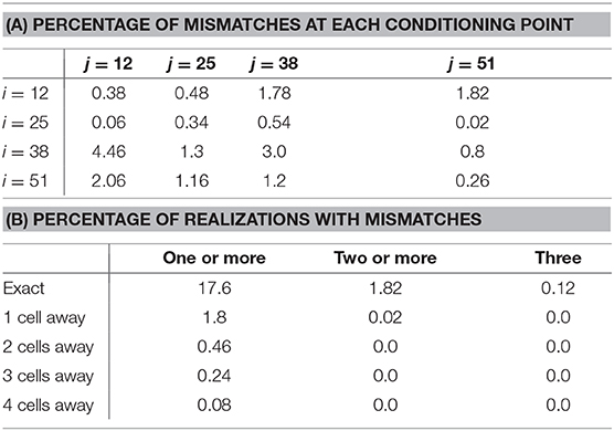
Table 2. Performance in honoring point conditioning.

FIGURE 12

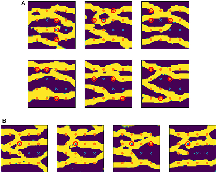
Figure 12. Realizations where conditioning failed. Orange dots indicate points conditioned to low permeability (0) and blue crosses indicate points conditioned to high permeability (1). Mismatches are circled in red. (A) Realizations containing 3 mismatches. (B) Realizations with large misplacement (4 cells away).

Note that mismatches do not occur using PCA parametrization (assuming an exact method for the eigendecomposition is used) as it is derived to explicitly preserve the spatial covariances. The presence of mismatches in our method reflects the approach that we take to parametrization: We formulate the parametrization by addressing the data generating process rather than the spatial statistics of the data, resulting in a parametrization that extrapolates to new realizations that, except for a few pixels/cells, are otherwise indistinguishable from data. In view of the good results from our flow experiments, the importance of honoring point conditioning precisely to the cell level could be argued. On the other hand, we also acknowledge that conditioning points are normally scarce and obtained from expensive measurements, so it is desirable that these be well honored in the parametrization.

4. Discussion and Practical Details

4.1. Practical Advantages of WGAN

An issue with the standard formulation of GAN is the lack of a convergence curve or loss function that is informative about the sample quality. We illustrate this in Figure 13 where we show the convergence curve of our trained WGAN model, and a convergence curve of a GAN using the standard formulation. We also show realizations generated by the models along the training process. The curve of WGAN follows the ideal behavior that is expected in an optimization process, whereas the curve of standard GAN is erratic and shows no correlation with the quality of the generated samples. We can also see another well-known issue of standard GAN which is the tendency to mode collapse, i.e., a lack of sample diversity, manifested as the repetition of only one or few image modes. We see that the standard GAN generator jumps from one mode solution to another. Note that in some cases, however, mode collapse is more subtle and not easily detectable. This is very problematic to our application since it can lead to biases in uncertainty quantification and unsuccessful history matching due to the absence of some modes in the generator.

FIGURE 13

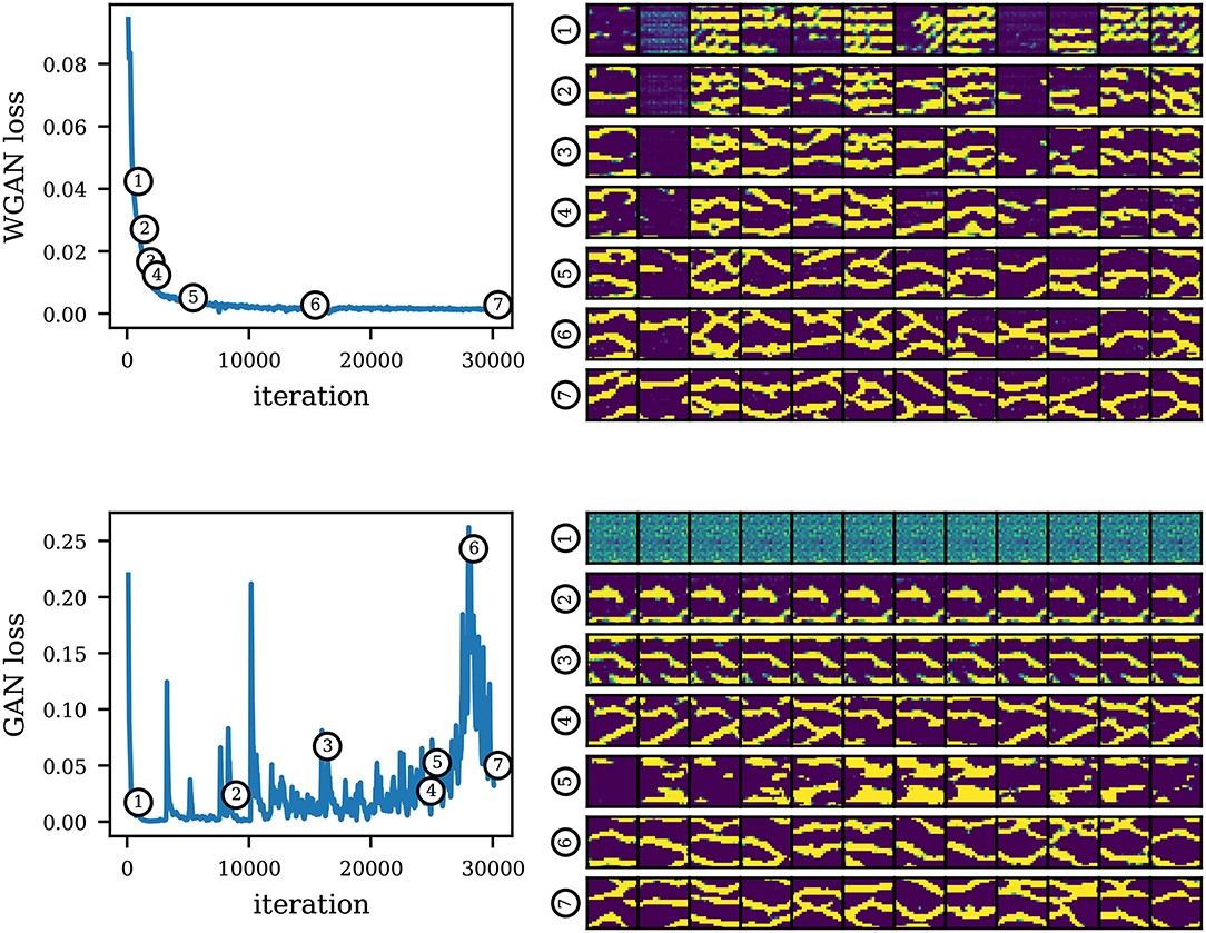
Figure 13. Convergence curves of a WGAN model (top) and a standard GAN model (bottom). On the right, we show realizations along the training of the corresponding models. We see that GAN loss is uninformative regarding sample quality. Note that the losses are not comparable between models since the formulations are different.

Given the lack of an informative convergence metric in standard GAN, the training process would involve a human judge serving as the actual loss function to track the visual quality along the training (in practice, weights are saved at several checkpoints and assessed after the fact). On top of this, the human operator would need to look at multiple realizations at once in an attempt to detect mode collapse. Clearly, this subjective process is error prone, not to mention labor intensive. In Figure 14 we show two standard GAN models and their flow responses in the unconditional uniform flow test case, based again on 5,000 realizations. On the top row, we show again the reference results (mean saturation and water breakthrough time) for comparison. We also compute the two-point probability function (Torquato and Stell, 1982) of the generated realizations (last column; we show the mean and one standard deviation). We see that in some cases, mode collapse is very evident and the model can be quickly discarded (second row). In other cases (last row), mode collapse is harder to detect and can lead to misleading predictions. We also see that the two-point probability function is not sufficient to detect mode collapse as this function does not measure the overall sample diversity.

FIGURE 14

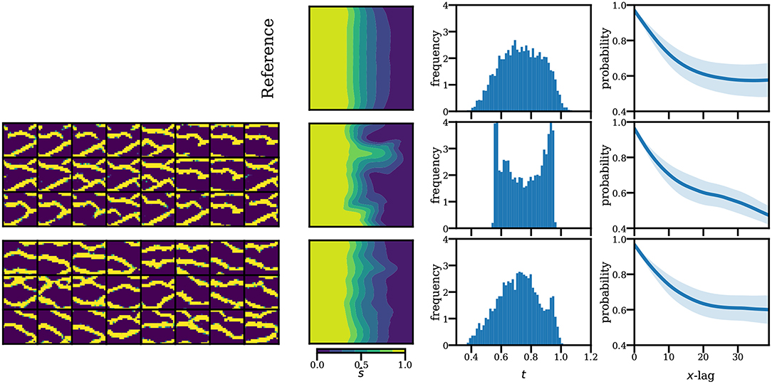
Figure 14. Examples of missing modes in standard GAN. Second and third rows show realizations generated by collapsing GAN models (left) and their responses (right). First row shows the reference solutions. The standard GAN was trained using the same generator architecture, but a ×4 larger discriminator than the one used in WGAN. We did not manage to find convergence with smaller discriminator sizes.

The Wasserstein formulation solves these issues by allowing the generator to minimize the Wasserstein distance between its distribution and the target distribution (Equation 5), therefore reducing mode collapse. Moreover, the Wasserstein distance is readily available in-training and can be used to assess convergence. Therefore, the Wasserstein formulation is better suited for automated applications, where robustness and a convergence criteria is essential.

4.2. Network Sizes Under Limited Data

As mentioned earlier, architecture design is largely problem-dependent and based on domain knowledge and heavy use of heuristics. The general approach is to start with a baseline architecture from a similar problem domain and tune it to accommodate for the present problem. Current computer vision applications use the pyramid architecture shown in Figure 2. These applications benefit from very large datasets of images. In contrast, our application uses a relatively small dataset. Recall that the discriminator D is trained using this limited dataset, therefore addressing the possibility of overfitting is important since the accuracy of D is crucial in the performance of the method. In particular, an overfitted D creates an issue where the Wasserstein estimate in section 5 is no longer accurate, making the gradients to the generator unreliable. We show the effect of overfitting in Figure 15A by training models with different discriminator sizes, and fixed generator architecture. We train discriminators of 2, 4, and 8 times the size of the discriminator used in our previous experiments. The way we increase the model size is by increasing the number of filters in each layer of the discriminator while keeping everything else constant. Another possibility is to add extra layers to the architecture. To detect overfitting, we evaluate the Wasserstein estimate using a separate validation set of 200 SNESIM realizations. We see that for an adequate size of the discriminator, the Wasserstein estimate as evaluated on either training or validation set are similar. However for larger models, the Wasserstein estimates on the training and validation sets start to wildly diverge as the optimization progresses, suggesting that the discriminator is overfitting and the estimates are no longer reliable. It is therefore necessary to adjust the size of the discriminator or use regularization techniques when data is very limited.

FIGURE 15

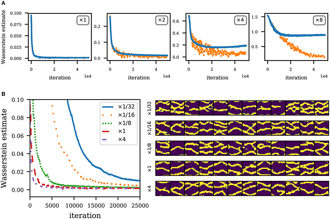
Figure 15. Performance of models with varying network sizes. (A) Convergence curve for different sizes of D (and fixed G). Solid blue lines indicate the training loss, and orange dotted lines indicate the validation loss. Note that the losses are not comparable across figures since the Lipschitz constants change with different D. (B) Left: Convergence curve for different sizes of G (and fixed D). Right: Realizations by generators of different sizes (at 15,000 iterations).

Regarding generator architectures, network sizes will in general be limited by compute and time resources; on the other hand, we only need just enough network capacity to be able to model complex structures. We illustrate this in Figure 15B where we train generators of different sizes (like before, we vary the number of filters in each layer) and fixed discriminator architecture. We train generators of $\frac{1}{32}$, $\frac{1}{16}$, $\frac{1}{8}$, and 4 times the size of the generator used in previous experiments. We also show realizations generated by each generator model after 15,000 training iterations. We see that for a very small network model ($\frac{1}{32}$), convergence is slow (as measured by iterations). Convergence is faster as the network size increases since it is easier to fit a larger network. Note, however, that the training iterations in larger networks are more expensive, possibly making convergence actually slower in terms of compute times. Therefore, there is diminishing returns in increasing the size of the generator.

4.3. GAN for Multipoint Geostatistical Simulations

In the domain of geology, a natural question is whether GANs can be directly applied as multipoint geostatistical simulators. This has been studied in a number of recent works (Mosser et al., 2017a,b; Laloy et al., 2018). The idea here is to use a single large training image and simply train a GAN model on patches of this image, instead of generating a dataset of realizations using an external multipoint geostatistical simulator. The result is a generator capable of generating patches of the image instead of the full-size training image. In order to recover the original size of the training image or to generate larger images, a simple trick is to feed an artificially expanded input array to the generator. This is illustrated in Figure 16A: If a generator has been trained with z of shape (n_z, 1, 1), we can feed the generator with expanded arrays of shape (n_z, n_y, n_x) (sampled from the higher dimensional analog of the same distribution) to obtain larger outputs. This is possible since we can still apply a convolving filter regardless of the input size. This is better illustrated with the 1D example shown in Figure 16B. In Figure 17, we show generated examples using this trick on our trained WGAN model, where we generate realizations of more than 10 times larger in each dimension (recall that our generator is trained on realizations of size 64 × 64). Whether this trick generalizes to arbitrarily large sizes (in the sense that the flow statistics are preserved) deserves further study.

FIGURE 16

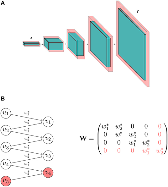
Figure 16. Examples of artificially expanding the input array to obtain a larger output. (A) Illustration of artificially expanding the input array in the generator network. Blue blocks represent the original state shapes that a normal input array follows in the generator. Light red blocks represent the new state shapes of an expanded input array. (B) 1D example of the artificial expansion and its associated matrix modification. Weights $w_1^{*},w_2^{*}$ are already trained. The expanded matrix can be obtained by appending an additional row and column.

FIGURE 17

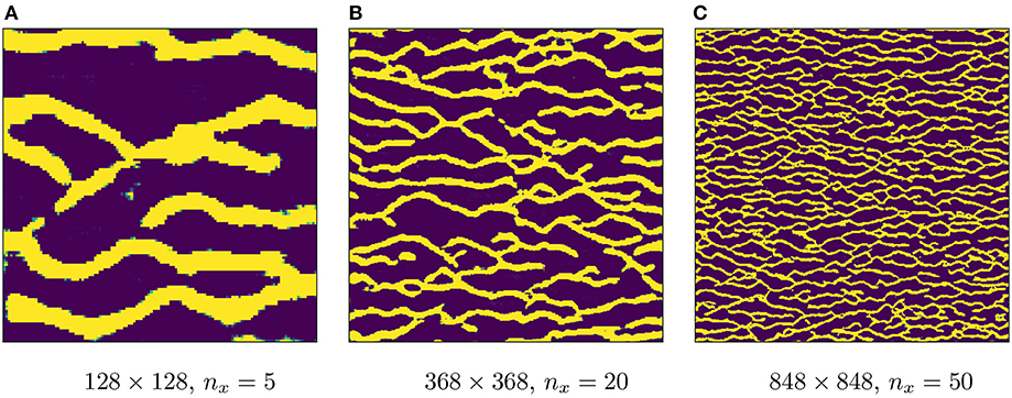
Figure 17. Artificially upscaled realizations by feeding an expanded input array. Images (evidently) not at scale. (A) 128 × 128, n_x = 5. (B) 368 × 368, n_x = 20. (C) 848 × 848, n_x = 50.

An important feature of multipoint geostatistical simulators is the ability to generate conditional realizations. Performing conditioning using unconditionally trained generators has been the focus of recent works. In Dupont et al. (2018) and Mosser et al. (2018b) conditioning was performed by optimization in the latent space using an image inpainting technique (Yeh et al., 2016). In Laloy et al. (2018) conditioning is imposed as an additional constraint in the inversion process. In our concurrent work (Chan and Elsheikh, 2018b), we propose a method based on stacking a second neural network to the generator that performs the conditioning.

5. Conclusions

We investigated generative adversarial networks (GAN) as a sample-based parametrization method of stochastic inputs in partial differential equations. We focused on parametrization of geological models which is critical in the performance of subsurface simulations. We parametrized conditional and unconditional permeability, and used the parametrization to perform uncertainty quantification and parameter estimation (history matching). Overall, the method shows very good results in reproducing the spatial statistics and flow responses, as well as preserving visual realism while achieving a dimensionality reduction of two orders of magnitude, from 64 × 64 to 30. In uncertainty quantification, we found that the method reproduces the high order statistics of the flow responses as seen from the estimated distributions of the saturation and the production. The estimated distributions show very good agreement and the modality of the distributions are reproduced. In parameter estimation, we found successful inversion results in both conditional and unconditional settings, and reasonable inversion results for challenging hand-crafted images. We also compared implementations of the standard formulation of GAN with the Wasserstein formulation, finding the latter to be more suitable for our applications. We discussed issues regarding network size under limited data, highlighting the importance of the choice of discriminator size to prevent overfitting. Finally, we also discussed using GANs for multipoint geostatistical simulations. Possible directions to extend this work include improving current GAN methods for limited data, and further assessments in other test cases.

Data Availability Statement

The datasets generated for this study are available on request to the corresponding author.

Author Contributions

SC was in charge of the writing and technical aspects of this work and performed all the numerical experiments. AE proposed the idea of using generative adversarial networks for geological parametrization.

Conflict of Interest

The authors declare that the research was conducted in the absence of any commercial or financial relationships that could be construed as a potential conflict of interest.

References

Aanonsen, S. I. (2005). “Efficient history matching using a multiscale technique,” in SPE Reservoir Simulation Symposium (The Woodlands: Society of Petroleum Engineers). doi: 10.2118/92758-MS

CrossRef Full Text | Google Scholar

Arjovsky, M., and Bottou, L. (2017). Towards principled methods for training generative adversarial networks. arxiv [Preprint] arXiv:1701.04862.

Arjovsky, M., Chintala, S., and Bottou, L. (2017). Wasserstein GAN. arxiv [Preprint] arXiv:1701.07875.

Google Scholar

Bergen, K. J., Johnson, P. A., Maarten, V., and Beroza, G. C. (2019). Machine learning for data-driven discovery in solid earth geoscience. Science 363:eaau0323. doi: 10.1126/science.aau0323

PubMed Abstract | CrossRef Full Text | Google Scholar

Berthelot, D., Schumm, T., and Metz, L. (2017). Began: Boundary equilibrium generative adversarial networks. arxiv [Preprint] arXiv:1703.10717.

Google Scholar

Bissell, R. (1994). “Calculating optimal parameters for history matching,” in ECMOR IV-4th European Conference on the Mathematics of Oil Recovery. doi: 10.3997/2214-4609.201411181

CrossRef Full Text | Google Scholar

Canchumuni, S. W., Emerick, A. A., and Pacheco, M. A. C. (2019). History matching geological facies models based on ensemble smoother and deep generative models. J. Petrol. Sci. Eng. 177:941–958. doi: 10.1016/j.petrol.2019.02.037

CrossRef Full Text | Google Scholar

Chan, S., and Elsheikh, A. H. (2017). Parametrization and generation of geological models with generative adversarial networks. arxiv [Preprint] arXiv:1708.01810.

Google Scholar

Chan, S., and Elsheikh, A. H. (2018a). A machine learning approach for efficient uncertainty quantification using multiscale methods. J. Comput. Phys. 354, 493–511. doi: 10.1016/j.jcp.2017.10.034

CrossRef Full Text | Google Scholar

Chan, S., and Elsheikh, A. H. (2018b). Parametric generation of conditional geological realizations using generative neural networks. arxiv [Preprint] arXiv:1807.05207.

Google Scholar

Chang, H., Zhang, D., and Lu, Z. (2010). History matching of facies distribution with the enkf and level set parameterization. J. Comput. Phys. 229, 8011–8030. doi: 10.1016/j.jcp.2010.07.005

CrossRef Full Text | Google Scholar

Chavent, G., and Bissell, R. (1998). “Indicator for the refinement of parameterization,” in Inverse Problems in Engineering Mechanics eds M. Tanaka and G. S. Dulikravich (Nagano: Elsevier), 309–314. doi: 10.1016/B978-008043319-6/50036-4

CrossRef Full Text | Google Scholar

Christie, M. A., and Blunt, M. (2001). “Tenth SPE comparative solution project: a comparison of upscaling techniques,” in SPE Reservoir Simulation Symposium (Houston, TX: Society of Petroleum Engineers). doi: 10.2118/66599-MS

CrossRef Full Text | Google Scholar

Coiffier, G., and Renard, P. (2019). “3d geological image synthesis from 2d examples using generative adversarial networks,” in Petroleum Geostatistics 2019, Vol. 2019 (European Association of Geoscientists & Engineers), 1–5. doi: 10.3997/2214-4609.201902198

CrossRef Full Text | Google Scholar

Dorn, O., and Villegas, R. (2008). History matching of petroleum reservoirs using a level set technique. Inverse Probl. 24:035015. doi: 10.1088/0266-5611/24/3/035015

CrossRef Full Text | Google Scholar

Dupont, E., Zhang, T., Tilke, P., Liang, L., and Bailey, W. (2018). Generating realistic geology conditioned on physical measurements with generative adversarial networks. arxiv [Preprint] arXiv:1802.03065.

Google Scholar

Fukushima, K., and Miyake, S. (1982). “Neocognitron: a self-organizing neural network model for a mechanism of visual pattern recognition,” in Competition and Cooperation in Neural Nets eds S. Amari, M. A. Arbib (Kyoto: Springer), 267–285. doi: 10.1007/978-3-642-46466-9_18

PubMed Abstract | CrossRef Full Text | Google Scholar

Gavalas, G., Shah, P., and Seinfeld, J. H. (1976). Reservoir history matching by bayesian estimation. Soc. Petrol. Eng. J. 16, 337–350. doi: 10.2118/5740-PA

CrossRef Full Text | Google Scholar

Goodfellow, I., Pouget-Abadie, J., Mirza, M., Xu, B., Warde-Farley, D., Ozair, S., et al. (2014). “Generative adversarial nets,” in Advances in Neural Information Processing Systems (Montreal, QC), 2672–2680.

Google Scholar

Graham, G. H., and Chen, Y. (2020). Bayesian inversion of generative models for geologic storage of carbon dioxide. arxiv [Preprint] arXiv:2001.04829.

Google Scholar

Grimstad, A., Mannseth, T., Naevdal, G., and Urkedal, H. (2001). “Scale splitting approach to reservoir characterization,” in SPE Reservoir Simulation Symposium (Houston, TX: Society of Petroleum Engineers). doi: 10.2118/66394-MS

CrossRef Full Text | Google Scholar

Grimstad, A.-A., Mannseth, T., Aanonsen, S. I., Aavatsmark, I., Cominelli, A., Mantica, S., et al. (2002). “Identification of unknown permeability trends from history matching of production data,” in SPE Annual Technical Conference and Exhibition (San Antonio, TX: Society of Petroleum Engineers). doi: 10.2118/77485-MS

CrossRef Full Text | Google Scholar

Grimstad, A.-A., Mannseth, T., Naevdal, G., and Urkedal, H. (2003). Adaptive multiscale permeability estimation. Comput. Geosci. 7, 1–25. doi: 10.1023/A:1022417923824

CrossRef Full Text | Google Scholar

Gulrajani, I., Ahmed, F., Arjovsky, M., Dumoulin, V., and Courville, A. C. (2017). “Improved training of Wasserstein gans,” in Advances in Neural Information Processing Systems (Long Beach, CA), 5769–5779.

He, K., Zhang, X., Ren, S., and Sun, J. (2016). “Deep residual learning for image recognition,” in Proceedings of the IEEE Conference on Computer Vision and Pattern Recognition (Las Vegas, NV), 770–778. doi: 10.1109/CVPR.2016.90

CrossRef Full Text | Google Scholar

Hornik, K., Stinchcombe, M., and White, H. (1989). Multilayer feedforward networks are universal approximators. Neural Netw. 2, 359–366. doi: 10.1016/0893-6080(89)90020-8

CrossRef Full Text | Google Scholar

Jacquard, P. (1965). Permeability distribution from field pressure data. Soc. Petrol. Eng. 5. doi: 10.2118/1307-PA

CrossRef Full Text | Google Scholar

Jafarpour, B., Goyal, V. K., McLaughlin, D. B., and Freeman, W. T. (2010). Compressed history matching: exploiting transform-domain sparsity for regularization of nonlinear dynamic data integration problems. Math. Geosci. 42, 1–27. doi: 10.1007/s11004-009-9247-z

CrossRef Full Text | Google Scholar

Jafarpour, B., and McLaughlin, D. B. (2007). Efficient permeability parameterization with the discrete cosine transform. Soc. Petrol. Eng. doi: 10.2118/106453-MS

CrossRef Full Text | Google Scholar

Jafarpour, B., and McLaughlin, D. B. (2009). Reservoir characterization with the discrete cosine transform. Soc. Petrol. Eng. 14. doi: 10.2118/106453-PA

CrossRef Full Text

Jahns, H. O. (1966). A rapid method for obtaining a two-dimensional reservoir description from well pressure response data. Soc. Petrol. Eng. 6. doi: 10.2118/1473-PA

CrossRef Full Text | Google Scholar

Jin, Z. L., Liu, Y., and Durlofsky, L. J. (2019). Deep-learning-based reduced-order modeling for subsurface flow simulation. arxiv [Preprint] arXiv:1906.03729.

Google Scholar

Kani, J. N., and Elsheikh, A. H. (2019). Reduced-order modeling of subsurface multi-phase flow models using deep residual recurrent neural networks. Transp. Porous Media 126, 713–741. doi: 10.1007/s11242-018-1170-7

CrossRef Full Text | Google Scholar

Karpathy, A. (2020). CS231n Convolutional Neural Networks for Visual Recognition. Availble online at: http://cs231n.github.io/convolutional-networks/

Khaninezhad, M. M., Jafarpour, B., and Li, L. (2012a). Sparse geologic dictionaries for subsurface flow model calibration: part I. Inversion formulation. Adv. Water Resour. 39, 106–121. doi: 10.1016/j.advwatres.2011.09.002

CrossRef Full Text | Google Scholar

Khaninezhad, M. M., Jafarpour, B., and Li, L. (2012b). Sparse geologic dictionaries for subsurface flow model calibration: part II. Robustness to uncertainty. Adv. Water Resour. 39, 122–136. doi: 10.1016/j.advwatres.2011.10.005

CrossRef Full Text | Google Scholar

Kingma, D., and Ba, J. (2014). Adam: a method for stochastic optimization. arxiv [Preprint] arXiv:1412.6980.

Google Scholar

Kodali, N., Abernethy, J., Hays, J., and Kira, Z. (2017). How to train your dragan. arxiv [Preprint] arXiv:1705.07215.

Laloy, E., Hérault, R., Jacques, D., and Linde, N. (2018). Training-image based geostatistical inversion using a spatial generative adversarial neural network. Water Resour. Res. 54, 381–406. doi: 10.1002/2017WR022148

CrossRef Full Text | Google Scholar

Laloy, E., Hérault, R., Lee, J., Jacques, D., and Linde, N. (2017). Inversion using a new low-dimensional representation of complex binary geological media based on a deep neural network. Adv. Water Resour. 110, 387–405. doi: 10.1016/j.advwatres.2017.09.029

CrossRef Full Text | Google Scholar

Laloy, E., Linde, N., Ruffino, C., Hérault, R., Gasso, G., and Jacques, D. (2019). Gradient-based deterministic inversion of geophysical data with generative adversarial networks: is it feasible? Comput. Geosci. 133:104333. doi: 10.1016/j.cageo.2019.104333

CrossRef Full Text | Google Scholar

Lassila, T., Manzoni, A., Quarteroni, A., and Rozza, G. (2014). “Model order reduction in fluid dynamics: challenges and perspectives,” in Reduced Order Methods for Modeling and Computational Reduction eds A. Quarteroni and G. Rozza (Springer), 235–273. doi: 10.1007/978-3-319-02090-7_9

CrossRef Full Text | Google Scholar

Liu, Y., and Durlofsky, L. J. (2019). Multilevel strategies and geological parameterizations for history matching complex reservoir models. SPE J. doi: 10.2118/193895-MS

CrossRef Full Text | Google Scholar

Liu, Y., Sun, W., and Durlofsky, L. J. (2019). A deep-learning-based geological parameterization for history matching complex models. Math. Geosci. 51, 725–766. doi: 10.1007/s11004-019-09794-9

CrossRef Full Text | Google Scholar

Lu, P., and Horne, R. N. (2000). “A multiresolution approach to reservoir parameter estimation using wavelet analysis,” In SPE Annual Technical Conference and Exhibition. Society of Petroleum Engineers, (Dallas, TX). doi: 10.2118/62985-MS

CrossRef Full Text | Google Scholar

Ma, X., and Zabaras, N. (2011). Kernel principal component analysis for stochastic input model generation. J. Comput. Phys. 230, 7311–7331. doi: 10.1016/j.jcp.2011.05.037

CrossRef Full Text | Google Scholar

Mallat, S. G. (1989). Multiresolution approximations and wavelet orthonormal bases of² (). Trans. Am. Math. Soc. 315, 69–87. doi: 10.2307/2001373

CrossRef Full Text | Google Scholar

Mariethoz, G., and Caers, J. (2014). Multiple-Point Geostatistics: Stochastic Modeling With Training Images. John Wiley & Sons.

Google Scholar

Miyato, T., Kataoka, T., Koyama, M., and Yoshida, Y. (2018). Spectral normalization for generative adversarial networks. arxiv [Preprint] arXiv:1802.05957.

Google Scholar

Moreno, D., and Aanonsen, S. I. (2007). “Stochastic facies modelling using the level set method,” in EAGE Conference on Petroleum Geostatistics (London).

Google Scholar

Mosser, L., Dubrule, O., and Blunt, M. (2018a). “Stochastic seismic waveform inversion using generative adversarial networks as a geological prior,” in First EAGE/PESGB Workshop Machine Learning (London). doi: 10.3997/2214-4609.201803018

CrossRef Full Text | Google Scholar

Mosser, L., Dubrule, O., and Blunt, M. J. (2017a). Reconstruction of three-dimensional porous media using generative adversarial neural networks. arxiv [Preprint] arXiv:1704.03225. doi: 10.1103/PhysRevE.96.043309

PubMed Abstract | CrossRef Full Text | Google Scholar

Mosser, L., Dubrule, O., and Blunt, M. J. (2017b). Stochastic reconstruction of an oolitic limestone by generative adversarial networks. arXiv:1712.02854. doi: 10.1007/s11242-018-1039-9

CrossRef Full Text | Google Scholar

Mosser, L., Dubrule, O., and Blunt, M. J. (2018b). Conditioning of three-dimensional generative adversarial networks for pore and reservoir-scale models. arxiv [Preprint] arXiv:1802.05622. doi: 10.3997/2214-4609.201800774

CrossRef Full Text | Google Scholar

Mosser, L., Dubrule, O., and Blunt, M. J. (2019). Deepflow: history matching in the space of deep generative models. arxiv [Preprint] arXiv:1905.05749.

Google Scholar

Mroueh, Y., Li, C.-L., Sercu, T., Raj, A., and Cheng, Y. (2017). Sobolev gan. arxiv [Preprint] arXiv:1711.04894.

Google Scholar

Oliver, D. S. (1996). Multiple realizations of the permeability field from well test data. SPE J. 1, 145–154. doi: 10.2118/27970-PA

CrossRef Full Text | Google Scholar

Qi, G.-J. (2017). Loss-sensitive generative adversarial networks on lipschitz densities. arxiv [Preprint] arXiv:1701.06264.

Google Scholar

Qin, T., Wu, K., and Xiu, D. (2019). Data driven governing equations approximation using deep neural networks. J. Comput. Phys. 395, 620–635. doi: 10.1016/j.jcp.2019.06.042

CrossRef Full Text | Google Scholar

Radford, A., Metz, L., and Chintala, S. (2015). Unsupervised representation learning with deep convolutional generative adversarial networks. arxiv [Preprint] arXiv:1511.06434.

Google Scholar

Razavi, S., Tolson, B. A., and Burn, D. H. (2012). Review of surrogate modeling in water resources. Water Resour. Res. 48. doi: 10.1029/2011WR011527

CrossRef Full Text | Google Scholar

Reynolds, A. C., He, N., Chu, L., and Oliver, D. S. (1996). Reparameterization techniques for generating reservoir descriptions conditioned to variograms and well-test pressure data. SPE J. 1, 413–426. doi: 10.2118/30588-PA

CrossRef Full Text | Google Scholar

Sahni, I., and Horne, R. N. (2005). Multiresolution wavelet analysis for improved reservoir description. SPE Reservoir Eval. Eng. 8, 53–69. doi: 10.2118/87820-PA

CrossRef Full Text | Google Scholar

Salimans, T., Goodfellow, I., Zaremba, W., Cheung, V., Radford, A., and Chen, X. (2016). “Improved techniques for training gans,” in Advances in Neural Information Processing Systems (Barcelona), 2234–2242.

Google Scholar

Sarma, P., Durlofsky, L. J., and Aziz, K. (2008). Kernel principal component analysis for efficient, differentiable parameterization of multipoint geostatistics. Math. Geosci. 40, 3–32. doi: 10.1007/s11004-007-9131-7

CrossRef Full Text | Google Scholar

Shirangi, M. G. (2014). History matching production data and uncertainty assessment with an efficient TSVD parameterization algorithm. J. Petrol. Sci. Eng. 113, 54–71. doi: 10.1016/j.petrol.2013.11.025

CrossRef Full Text | Google Scholar

Shirangi, M. G., and Emerick, A. A. (2016). An improved TSVD-based Levenberg-Marquardt algorithm for history matching and comparison with Gauss-Newton. J. Petrol. Sci. Eng. 143, 258–271. doi: 10.1016/j.petrol.2016.02.026

CrossRef Full Text | Google Scholar

Simonyan, K., and Zisserman, A. (2014). Very deep convolutional networks for large-scale image recognition. arxiv [Preprint] arXiv:1409.1556.

Google Scholar

Strebelle, S. B., and Journel, A. G. (2001). “Reservoir modeling using multiple-point statistics,” in SPE Annual Technical Conference and Exhibition (New Orleans, LA: Society of Petroleum Engineers). doi: 10.2118/71324-MS

CrossRef Full Text | Google Scholar

Sun, A. Y., and Scanlon, B. R. (2019). How can big data and machine learning benefit environment and water management: a survey of methods, applications, and future directions. Environ. Res. Lett. 14:073001. doi: 10.1088/1748-9326/ab1b7d

CrossRef Full Text | Google Scholar

Tarakanov, A., and Elsheikh, A. H. (2019). Regression-based sparse polynomial chaos for uncertainty quantification of subsurface flow models. J. Comput. Phys. 399:108909. doi: 10.1016/j.jcp.2019.108909

CrossRef Full Text | Google Scholar

Tavakoli, R., and Reynolds, A. C. (2009). “History matching with parametrization based on the SVD of a dimensionless sensitivity matrix,” in SPE Reservoir Simulation Symposium (The Woodlands, TX: Society of Petroleum Engineers). doi: 10.2118/118952-MS

CrossRef Full Text | Google Scholar

Tavakoli, R., and Reynolds, A. C. (2011). Monte Carlo simulation of permeability fields and reservoir performance predictions with SVD parameterization in RML compared with EnKF. Comput. Geosci. 15:99–116. doi: 10.1007/s10596-010-9200-8

CrossRef Full Text | Google Scholar

Tieleman, T., and Hinton, G. (2012). Lecture 6.5, RMSPROP: Divide the gradient by a running average of its recent magnitude. COURSERA Neural Netw. Mach. Learn. 4.

Torquato, S., and Stell, G. (1982). Microstructure of two–phase random media. I. The n-point probability functions. J. Chem. Phys. 77, 2071–2077. doi: 10.1063/1.444011

CrossRef Full Text | Google Scholar

Vasilyeva, M., and Tyrylgin, A. (2018). Machine learning for accelerating effective property prediction for poroelasticity problem in stochastic media. arxiv [Preprint] arXiv:1810.01586.

Google Scholar

Vo, H. X., and Durlofsky, L. J. (2016). Regularized kernel PCA for the efficient parameterization of complex geological models. J. Comput. Phys. 322, 859–881. doi: 10.1016/j.jcp.2016.07.011

CrossRef Full Text | Google Scholar

Wierstra, D., Schaul, T., Glasmachers, T., Sun, Y., Peters, J., and Schmidhuber, J. (2014). Natural evolution strategies. J. Mach. Learn. Res. 15, 949–980. doi: 10.5555/2627435.2638566

CrossRef Full Text | Google Scholar

Wierstra, D., Schaul, T., Peters, J., and Schmidhuber, J. (2008). “Natural evolution strategies,” in Evolutionary Computation, 2008. CEC 2008, IEEE World Congress on Computational Intelligence (Hong Kong: IEEE), 3381–3387. doi: 10.1109/CEC.2008.4631255

CrossRef Full Text | Google Scholar

Yeh, R., Chen, C., Lim, T. Y., Hasegawa-Johnson, M., and Do, M. N. (2016). Semantic image inpainting with perceptual and contextual losses. arxiv [Preprint] arXiv:1607.07539. doi: 10.1109/CVPR.2017.728

CrossRef Full Text | Google Scholar

Zhang, T., Tilke, P., Dupont, E., Zhu, L., Liang, L., Bailey, W., et al. (2019). “Generating geologically realistic 3d reservoir facies models using deep learning of sedimentary architecture with generative adversarial networks,” in International Petroleum Technology Conference (Beijing). doi: 10.2523/IPTC-19454-MS

CrossRef Full Text | Google Scholar

Zhong, Z., Sun, A. Y., and Jeong, H. (2019). Predicting co2 plume migration in heterogeneous formations using conditional deep convolutional generative adversarial network. Water Resour. Res. 55, 5830–5851. doi: 10.1029/2018WR024592

CrossRef Full Text | Google Scholar