Development of end-to-end low-cost IoT system for densely deployed PM monitoring network: an Indian case study

Particulate matter (PM) is considered the primary contributor to air pollution and has severe implications for general health. PM concentration has high spatial variability and thus needs to be monitored locally. Traditional PM monitoring setups are bulky, expensive, and cannot be scaled for dense deployments. This paper argues for a densely deployed network of IoT-enabled PM monitoring devices using low-cost sensors, specifically focusing on PM10 and PM2.5, the most health-impacting particulates. In this work, 49 devices were deployed in a region of the Indian metropolitan city of Hyderabad, of which 43 devices were developed as part of this work, and six devices were taken off the shelf. The low-cost sensors were calibrated for seasonal variations using a precise reference sensor and were particularly adjusted to accurately measure PM10 and PM2.5 levels. A thorough analysis of data collected for 7 months has been presented to establish the need for dense deployment of PM monitoring devices. Different analyses such as mean, variance, spatial interpolation, and correlation have been employed to generate interesting insights about temporal and seasonal variations of PM10 and PM2.5. In addition, event-driven spatio-temporal analysis is done for PM2.5 and PM10 values to understand the impact of the bursting of firecrackers on the evening of the Diwali festival. A web-based dashboard is designed for real-time data visualization.

1 Introduction

Air pollution has been an issue of grave concern across the world for decades (COMEAP, 2010). Particulate matter (PM) occurring from local activities significantly contributes to air pollution, which causes serious health implications. The average concentration of PM2.5 and PM10 in India is 55.8 μ g/m³ and 131 μ g/m³, 11 times higher than the WHO guideline (Greenstone et al., 2022). According to an estimate, in 2019, around 6.7 million premature deaths globally were associated with air pollution (Fuller et al., 2022). Studying and continuously monitoring the various patterns related to air pollution is essential to address the challenge comprehensively.

1.1 Existing approaches and related works

Many countries have established elaborate structures for air-quality monitoring based on beta attenuation monitor (BAM) and tapered element oscillating microbalance (TEOM) often deployed by pollution control boards and other governmental agencies to monitor air quality (Khot and Chitre, 2017). For example, the metropolitan city of Hyderabad in India, where this study is based has 12 centralized air quality monitoring stations (AQMS). Not only precise measuring techniques like BAM and TEOM but several recent studies have been conducted to monitor air quality using low-cost sensors (Piedrahita, 2014; Clements et al., 2017). The importance of setting precise performance targets for PM2.5 sensors is further supported in the context of low-cost sensor accuracy and reliability, as discussed in Williams et al. (2019), indicating a critical area of focus for urban air quality monitoring networks. Moreover, internet-of-things (IoT) and cloud computing have been used for real-time PM monitoring. Citywide deployment of such devices has been studied to increase pollution data’s spatial-temporal resolution. For instance, in Cheng et al. (2019), 1,000 devices were deployed for 10 months in Beijing, China (area 16, 411 km²). In Lu et al. (2021), 361 devices were deployed for 1 year in a large area of 1302 km² in Los Angeles, California, to estimate hourly intra-urban PM2.5 distribution patterns using machine learning model. In Zhao et al. (2019), 169 devices were deployed in 20 km × 20 km area measuring PM2.5 every hour with a focus on identifying the primary source of PM2.5. In Montrucchio et al. (2020), 100 devices have been deployed, both stationary and mobile, for 5 months in Turin, Italy. In Becnel et al. (2019), 50 devices have been deployed in a large area of 100 km² for 6 months in Utah, United States, discussing the reliability and efficiency of low-cost PM sensors for spatial and temporal dense heterogeneous pollution data. In Gupta et al. (2018), 20 devices were deployed in Los Angeles, California, to quantify the impact of wildfires in California by using 20 low-cost air quality monitoring devices and satellite data. Similarly, in Penza et al. (2017), 11 devices were deployed in Bari, Italy, discuss the deployment challenges and solutions of these sensors in urban settings. In Lee et al. (2019), 438 devices were deployed for 2 months in Taichung, Taiwan (area 163 km²). In Park et al. (2019), 30 devices were deployed in an area of 800 m × 800 m discussing the suitability of low-cost sensors for networks of air quality monitors for dense deployment, but the data collection is significantly less. In Popoola et al. (2010), authors deployed a network of 45 low-cost electrochemical sensor devices in and around Cambridge, United Kingdom, for 2.5 months. The network provided measurements of harmful gases (CO, NO, NO₂), temperature, and relative humidity (RH). The collected data from these devices was analyzed for source attribution. The authors also determined the regional pollution level by studying variations in the sensor readings deployed in different environments. In Brienza et al. (2015), authors developed a low-cost device named uSense, which can measure the concentration of harmful gases (NO₂, O3, CO) in the ambient environment. It uses Wi-Fi to offload the sensed data on a cloud server. Wi-Fi connectivity enables users to place the device indoors or outdoors in balconies or gardens.

1.2 Limitations and identified research gaps

Despite the advancements in air quality monitoring, there are still significant gaps in the research. The primary issue is that, although the air quality monitoring apparatus like AQMS, BAM, TEOM are very accurate but they are often expensive, bulky, and large in size (Yi et al., 2015). Thus, they cannot be densely deployed, leading to a significant mismatch between the requirement of PM2.5 and PM10 data and its availability. Consequently, the resolution of available air quality data is limited as very few stations are typically responsible for an entire city region. For example, in a big metropolitan city like Hyderabad, with a population of over 6.7 million (Census India, 2011) and area over 650 km², the Central Pollution Control Board (CPCB) and the Telangana State Pollution Control Board (TSPCB) have deployed only 12 (AQMS) (CPCB India, 2015). This low resolution is insufficient for a deeper understanding of PM2.5 and PM10, as pollutant levels can vary drastically even within smaller blocks in a city (Apte et al., 2017).

For localized monitoring and real-time analysis of outdoor PM (PM2.5 PM10) and improving the spatial and temporal resolution of the data, a dense IoT system is needed to send more data points. Frequent sensing of air pollution data through transmitting multiple data points improves spatial and temporal resolution. It aids in source identification, identifying pollution patterns, and assessing mitigation measures. Moreover, a significant proportion of the monitoring devices in operation today require consistent calibration. Any deviations in calibration practices can undermine the integrity of the data. Thus, consistent calibration of affordable sensors is vital to guarantee data reliability (Popoola et al., 2010; Lewis and Edwards, 2016). The necessity for such rigorous calibration and validation, especially under varying environmental conditions, is further underscored in Borrego and et al. (2018). Air quality data often is not integrated with other relevant data, such as traffic flow, ongoing construction activities, or season/event-specific variations. Such integrations can offer a more holistic understanding of pollution sources and patterns (Chen et al., 2014; Kumar, 2015). The data collated through such methodologies allows for the immediate detection of pollution spikes and changes, helps understand long-term trends and seasonal variations, makes more accurate predictions, and evaluates the impact of interventions, which is scalable with low-cost portable ambient sensors. However, current research and practices have not adequately addressed this need, which represents a significant research gap. Despite the technological advancements in air quality monitoring, there remain pronounced challenges, especially in densely populated urban environments like Hyderabad. The limited presence of AQMS, while precise, cannot fully capture the multifaceted air quality variations in large urban landscapes. The evident need for dense deployment, the challenge of consistent calibration, and the integration of diverse data sources underscore the existing research gaps. Our study aims to bridge some of these voids. By concentrating on dense deployment of calibrated IoT devices, we aim to enhance data resolution and provide a more nuanced understanding of air quality variations.

1.3 Contributions

In our preliminary work (Reddy et al., 2020), a smaller network with ten devices was deployed inside the International Institute of Information Technology Hyderabad (IIITH) campus for PM2.5 PM10 monitoring. Field experience from this deployment highlighted the need for a denser deployment across different environments and areas with calibrated PM (PM2.5 PM10) sensor and a more robust device that can cache data to avoid data loss due to communication outages. In this paper, an end-to-end low-cost IoT system is developed and densely deployed for monitoring PM2.5 PM10 with fine spatio-temporal resolution. The system includes designing the hardware, calibrating the low-cost sensors, cloud interfacing, and developing a web-based dashboard.

The specific contributions of this paper are:

1. For the high spatial resolution of outdoor PM2.5 PM10, 49 IoT-based PM monitoring devices were developed, calibrated, and deployed at various outdoor locations.

2. The developed device is designed to be robust against the issue of data loss due to connection and power outages. The device maintains an offline cache in the event of an outage. The stored data is offloaded in bulk once the power and communication are restored.

3. All PM sensors were calibrated for seasonal variations by co-locating with a reference sensor. Also, each device was calibrated individually.

4. The devices were deployed at 49 outdoor locations covering a 4 km² area in Gachibowli, Hyderabad, India. The field locations were selected to include urban, semi-urban, and green regions. Few devices were deployed at busy traffic junctions and roadsides. The data was recorded at a frequency of every 30 s (sec), spanning over all the seasons for 7 months, thus aggregating 20.7 million data points.

5. A web-based dashboard was developed and deployed to visualize the data in real time.

6. Different analyses were carried out by observing seasonal mean and variance, spatial interpolation, event-driven variation, and correlation. Results show the optimal deployment across a varied landscape and can be a key factor in identifying the release of high concentration in real-time.

Our work differs significantly from the previous studies discussed earlier (Popoola et al., 2010; Brienza et al., 2015; Gupta et al., 2018; Becnel et al., 2019; Cheng et al., 2019; Lee et al., 2019; Park et al., 2019; Zhao et al., 2019; Montrucchio et al., 2020; Lu et al., 2021) and also shown in Table 1. For example (Popoola et al., 2010; Brienza et al., 2015), are about gas monitoring, while this paper focuses mainly on PM monitoring. The studies in (Gupta et al., 2018; Becnel et al., 2019; Cheng et al., 2019; Zhao et al., 2019; Montrucchio et al., 2020; Lu et al., 2021) have a large number of devices for citywide monitoring of PM but have a sparse deployment ($<$ 0.6 devices per km²) in contrast to our dense deployment ($>$ 12 devices per km²). The work in Lee et al. (2019); Park et al. (2019) is on dense deployment, but in Lee et al. (2019) ($<$ 2.6 devices per km²) for a small duration of 2 months which is very less for a comprehensive seasonal analysis. The network in Park et al. (2019) is not an IoT network. Data is collected locally on microSD card for a small duration, while our work involves an IoT network deployed for the last 1 year collecting large data sets.

TABLE 1

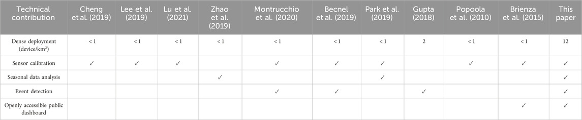
TABLE 1. Comparison of work done in this paper with other papers in the literature.

The rest of the paper is structured as follows: Section 2 describes the complete system’s hardware architecture and software design. Section 3 describes the measurement setup and the deployment plan. Section 4 describes the process of data collection, preprocessing, and calibration. Section 5 presents the development of the dashboard and its framework. Section 6 presents the observations from the measurement campaign. Finally, the conclusions are deduced and articulated in Section 7.

2 Hardware architecture: General overview and specifications

2.1 Hardware specification

Figure 1 shows the hardware architecture and circuit board for the developed PM monitoring device in this work. The basic architecture consists of sensors (PM sensor SDS011 and temperature humidity sensor SHT21), a communication module (SIM800L and eSIM), a real-time clock (RTC), and a lithium polymer (LiPo) battery.

FIGURE 1

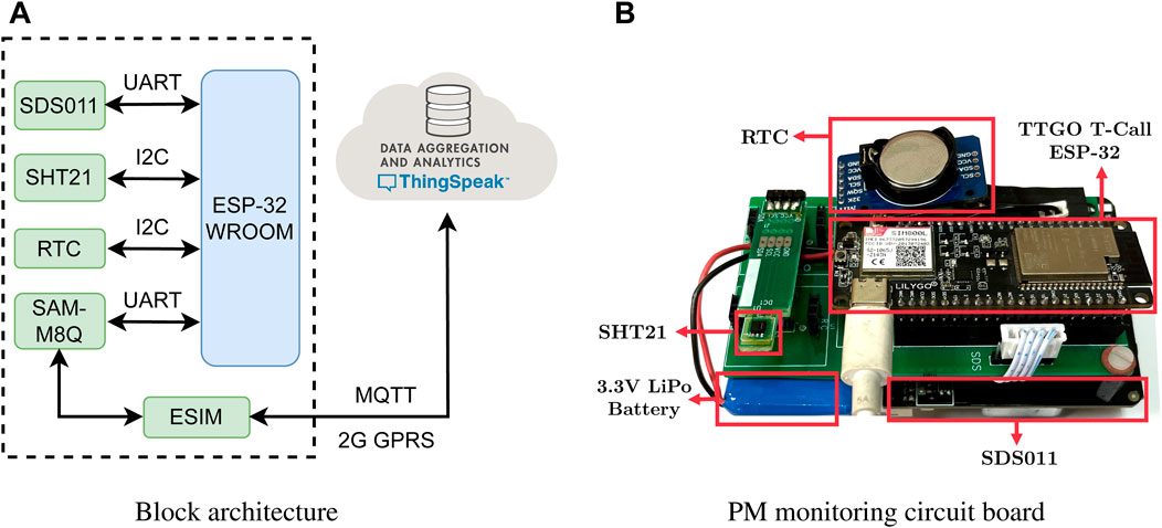
FIGURE 1. Block architecture and the circuit board of the deployed PM monitoring device. (A) Block architecture, (B) PM monitoring circuit board.

All these components are connected to the microcontroller TTGO T-Call ESP32. The controller reads data from all the sensors periodically every 30 s and offloads it to ThingSpeak, a cloud-based server employing message queuing telemetry transport secured (MQTTS) over a 2G or Wi-Fi network. The data packet size is 28 bytes. The device is powered with an AC-DC power adapter and a 1,000 mAh battery and enclosed in an IP65 box made of ABS filament; the enclosure offers complete protection against dust and good protection against water. The form dimensions are width = 125 mm, depth = 125 mm, and height = 125 mm. The SDS011 and SIM800L modules are connected to the controller through the UART protocol, while the SHT21 and RTC are connected through the I2C protocol. The overall cost of the device after adding the cost of individual hardware components is 7000 INR (approximately 84 USD)¹. The specifications of the individual hardware components are listed in Table 2. The details of each component are given below.

TABLE 2

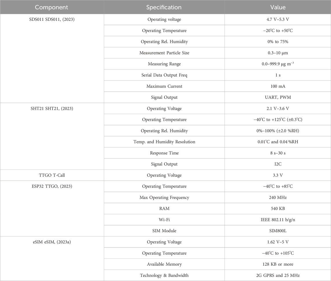
TABLE 2. Specifications of the components used in the developed PM monitoring device.

2.1.1 Nova SDS011

A Nova-SDS011 PM sensor (SDS011, 2023) is used in this study to gauge the presence and concentration of tiny particles with a diameter 10 µm or less (referred to as PM10) and particles with a diameter 2.5 µm or less (referred as PM2.5). The sensor uses light scattering phenomena to sense particle concentration. It is a low-cost sensor with a good correlation with BAM for PM2.5 PM10 monitoring (Badura et al., 2018). At the same time, it can achieve low error values after calibrating and using a simple linear regression (Patwardhan et al., 2021). Table 3 effectively demonstrates the high level of accuracy achieved by the Nova-SDS011 PM sensor in this study compared to other literature.

TABLE 3

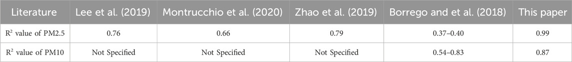
TABLE 3. Comparison of R² values for PM2.5 and PM10 in this paper with other papers in the literature.

2.1.2 SHT21

At high temperature and RH levels, light scattering-based PM (PM2.5 PM10) sensors do not operate reliably (Hernandez et al., 2017). Therefore, temperature-humidity sensor SHT21 (SHT21, 2023) is installed in the developed device to measure temperature and RH for filtering out any unreliable PM2.5 PM10 values.

2.1.3 Battery/power adapter

The developed device uses a 3.3 V rechargeable 1,000 mAh LiPo battery. A battery management circuit onboard the micro-controller module and a dedicated AC-to-DC power adapter charges the battery. If the AC input is available, the device will work using an AC-to-DC power adapter and charge the battery. It will switch automatically to battery power if no AC input is available. Including a battery in the system serves as a contingency measure to mitigate the impact of disruptions or power outages in the AC supply. The battery ensures uninterrupted data collection and device operation during such events.

2.1.4 TTGO T-Call ESP32

In field deployment, a wireless module is needed to send the sensed data to the cloud. This study uses the TTGO T-Call ESP-32 (TTGO, 2023), a Wi-Fi and SIM800L GSM/GPRS module with built-in Bluetooth wireless capabilities. Each device is configured to use Wi-Fi or GPRS according to the network availability in the area.

2.1.5 Cellular network

In the previous deployment on the campus, Reddy et al. (2020), Wi-Fi routers were used to communicate sensed data to the ThingSpeak server. However, Wi-Fi connectivity is unavailable at most locations outside the campus, particularly on the roadsides. In such places, we have used a 2G network, which has excellent coverage in the city. Since the sensed data is small in packet size (24 bytes), a 2G network data rate is sufficient. Moreover, the use of removable SIM cards in-field deployment gives rise to the threat of their misuse in case of theft. Hence an embedded SIM (eSIM) customized for IoT applications from the Sensorise service provider is used in the device (eSIM, 2023a). An eSIM is a small chip embedded in the hardware setup with the help of the SIM 800L module (eSIM, 2023b), thus restricting the reusability by the general public. IoT devices planned for long-term projects and having a field deployment are protected from the impact of evolving network technologies or service terminations by eliminating technical or carrier lock-ins with a single eSIM. The eSIM information is rewritable, making it easy to change the operator at any time. It allows users to change the service provider over the air without physically changing the eSIM. The Sensorise eSIM also provides the facility of multi-operator subscriptions. If there is an issue with one network, eSIMs can switch to other operators to connect to the network.

2.1.6 ThingSpeak

In the deployed IoT network, the data is aggregated at ThingSpeak, a cloud-based platform for IoT applications. It facilitates data access, logging, and retrieval by providing an application programming interface (API) (ThingSpeak, 2023). While personal servers can also be used for IoT applications, setting up and maintaining a personal server can be more complex than using a cloud-based platform like ThingSpeak, and it may require more technical expertise. Moreover, ThingSpeak supports many communication protocols, including MQTTS, with security and ease of scaling. In Ihita et al. (2021), the authors conducted a security analysis of AirIoT, an air-quality monitoring network, and proposed solutions for baseline security of any smart city air monitoring network. The paper recommended using MQTTS instead of MQTT as the latter does not provide data integrity, while attackers can access information such as payload, topic names, and IP addresses. MQTTS is a lightweight, publish-subscribe messaging protocol designed specifically for efficient communication in the context of IoT, where devices have limited processing power, memory, and battery life. Therefore, the MQTTS protocol is implemented in this work for communication between the device and ThingSpeak.

In our examination of low-cost consumer-grade monitors available in the Indian market, we identified a range of devices with varying price points. The AirIoT stands out as the most affordable option, retailing at ₹ 7,000. In contrast, the Prana CAAQMS Prana (2023) is on the higher end of the spectrum, priced at ₹ 64,900. Falling between these extremes are the Airveda (2023) and Atmotube PRO Atmo (2023), which are available for ₹ 35,000 and ₹ 15,000, respectively. Such a diverse price range underscores the accessibility and variability of air quality monitoring solutions for Indian consumers.

2.2 Working mechanism of the device

Figure 2 illustrates the flowchart of the sensing algorithm developed to avoid data loss in the event of a connection outage. The microcontroller first reads the sensed data every 30 s; however, the time to offload the sensed data depends upon the network. Next, the controller checks the network connectivity for pushing the data to the server. If the network is available, the data is transmitted instantaneously. However, if the network is unavailable, the data is stored locally in a part of the microcontroller RAM until the device reconnects to the network. Note that the size of microcontroller RAM is 540 KB, and part of it is used for code and header files (created while pushing data), while part of the remaining memory can be used to store data. We define S = 20,000 as the maximum number of data points that can be stored. Every stored data point contains the value of sensed parameters and the sensing time. Once the connection is restored, the stored data is uploaded to the cloud server in a bulk transmission and cleared from the device. In the case device memory is filled with back-logged data in the event of a prolonged connection outage, i.e., if the number of stored data points (s) is equal to the S, the data is cleared in first-in-first-out (FIFO) format to make space for the new incoming data.

FIGURE 2

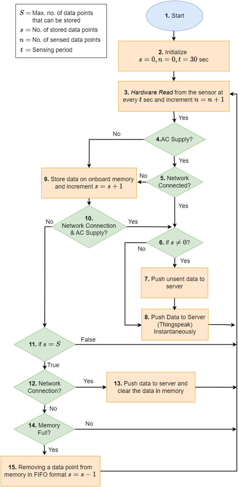
FIGURE 2. Working mechanism of the device.

3 Deployment strategy

Figure 3A shows the plan for the field deployment of devices, while Figure 3B shows an example of the deployed device at one of the locations. The deployment was done in the Gachibowli region of Hyderabad, the capital city of the Telangana state and the fourth largest populated city in India (Census India, 2011). A total of 49 devices were deployed in a region of approximately 4 km² to understand the variation of PM2.5 PM10 across different environments and areas.

FIGURE 3

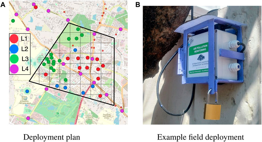
FIGURE 3. Deployment plan covering urban, semi-urban, green region, junctions, and roadsides poles. (A) Deployment plan, (B) Example field deployment.

Based on the landscape pattern of Gachibowli (Robert et al., 1996; Chakraborti et al., 2017), the entire region is divided into three categories: urban, semi-urban, and green. A few devices have also been deployed at busy traffic junctions and roadsides. Figure 3A shows the deployment plan of all the devices with exact locations of the following location types:

• Location type L1: Urban region

• Location type L2: Semi-urban region

• Location type L3: Green region

• Location type L4: Traffic junctions and roadsides poles

The 4 km² area has been divided into approximately 42 boxes. Every square box in Figure 3A represents an area of 400 × 400 m². An attempt has been made to deploy one device in each box depending on the availability of power, network, and consent availability. However, more than one device has been deployed in some boxes, as shown in Figure 3A. The field deployment of devices was completed in July 2021, and the data collection started in Aug. 2021. As part of experimentation, along with the devices developed at IIITH, a few devices from an Indian manufacturer, Airveda, were also deployed (Airveda, 2023). Table 4 summarizes all the deployed devices with their network configuration.

TABLE 4

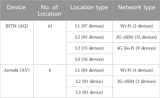
TABLE 4. Deployment setup.

4 Data collection, preprocessing, and calibration

Figure 4 shows a flow diagram depicting different steps in collecting useable data for analysis. It involves data collection, creating the dataset, removing outliers, and interpolating missing data, followed by calibration. Each of the steps involved is explained in detail.

FIGURE 4

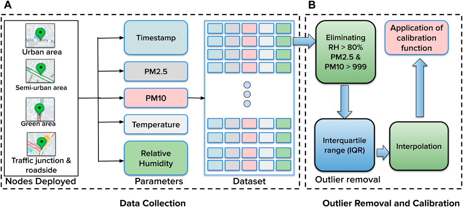
FIGURE 4. Data collection, preprocessing, and calibration. (A) Data Collection, (B) Outlier Removal and Calibration.

4.1 Data collection

To create the data set, the air quality was sensed at a frequency of t = 30 s for 43 IIITH devices. For 6 Airveda devices, t = 1 s, averaged over 30 s.

All the devices were deployed for almost 1 year and are still deployed. However, useable data were collected for 7 months (Aug. 2021, Nov. 2021, Dec. 2021, Jan. 2022, Apr. 2022, May 2022, and June 2022). The loss in the data is because the devices had to be brought back to the lab due to the frequent failure of low-cost sensors requiring regular repair and maintenance. Additionally, the devices were brought for seasonal calibration at regular intervals and to make a major upgrade in using ThingSpeak from MQTT to MQTTS (in Mar. 2022). A total of 20.70 million useable data points have been collected. As shown in Figure 4A, the collected dataset has PM2.5, PM10, temperature, and RH parameters. All the concentration values of PM10 and PM2.5 are mentioned in μg m⁻³ hereafter. The temperature and RH values are mentioned in °C and %, respectively. Corresponding to every device, a vector of data points sent from the device is stored on the cloud server for each sensing instance having the following elements:

• created_at: Timestamp at which the sensor value is read. This timestamp is recorded utilizing the RTC module of the device.

• PM10: Raw concentration of PM10 read by SDS011.

• PM2.5: Raw concentration of PM2.5 read by SDS011.

• RH: Raw RH value read by SHT21

• Temp: Raw temperature value read by SHT21 sensor.

The size of this payload (or sensor data sent from the device) for each sensing instance is 24 bytes. In addition to this, the following static information is stored in the cloud server.

• Device_id: ID for device identification like IIITH device as AQ-XX and Airveda device as AV-XX, where XX denotes the device sequence number.

• Location: Latitude and longitude according to the deployment location.

4.2 Data preprocessing

The following methods have been employed for preprocessing the raw data received from the PM monitoring device:

4.2.1 Outlier removal

Environmental conditions like RH and temperature, sensor behavior, and anthropogenic activities occasionally result in outliers in the sensed data. Hence the raw data received from the devices need to be preprocessed to make it statistically significant, as shown in Figure 4B. PM10 values are unreliable at higher RH levels (RH$>$80%). Also, errors may cause raw values to be out of the PM (PM2.5 PM10) sensor range (0-999). These unreliable points are thus removed. In the dataset, nearly 0.5% values have been found unreliable.

Further, to identify and remove outliers, the interquartile range (IQR) method (Dodge, 2008) is used. This method separates the data into four equal parts, which are sorted in ascending order using three quartiles (Q₁, Q₂ (median), Q₃). Let the difference between the first (Q₁) and the third quartile (Q₃) be represented by the I_QR, which is a measure of dispersion. A decision range is set to detect outliers with this approach, and every data point that falls outside this range is deemed an outlier. The lower and upper values in the range are given in Eqs 1, 2.

$L_r=Q_1-1.5I_{QR},(1)$

$U_r=Q_3+1.5I_{QR}.(2)$

Any data point less than the L_r or more than the U_r is called an outlier. In the collected dataset, nearly 1.4% values have been found as an outlier.

4.2.2 Interpolation

Interpolation is a technique to estimate the missing (or removed) data point between two existing data points. In the data set, only 1.9% data is an outlier which is very less and easy to interpolate. In this work, simple linear interpolation was used for this purpose.

4.3 Calibration

For calibration, the low-cost PM (PM2.5 PM10) sensors were co-located with a reference sensor [Aeroqual S500 (AeroqualS500, 2023; Aeroqual, 2023)] in a ventilated room for a week. Data points were collected at a frequency of 30 s. A raw dataset of approximately 20,160 data points for each sensor was collected to perform the calibration. Figure 5A shows the time series plot of PM10 averaged hourly for a few devices before deployment in the field. It can be observed that all the sensors follow the reference sensor in trend but differ with an offset in absolute value. Therefore, there is a need for calibration. It can also be observed that the offsets for each sensor are different. Although not shown to maintain brevity, the same is valid for raw PM2.5 values.

FIGURE 5

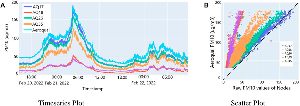
FIGURE 5. Time series and scatter plot of raw PM10 data (1-h average). (A) Timeseries Plot, (B) Scatter Plot.

This paper uses simple linear regression to compensate for the difference between the low-cost and reference sensor values. Although many complex algorithms have been used in the past for calibration, linear regression has been chosen since it can compensate for the offset well while preserving the trend in the data, as shown in our previous work for SDS011 in Patwardhan et al. (2021). The calibrated data y(i) corresponding to the i^th data point can be written as shown in Eq 3.

$y\left(i\right)=mx\left(i\right)+c,(3)$

where x(i) is the i^th raw data point and m, c are the learned parameters. Each sensor will have a different value of m and c.

Figure 6A shows the calibrated data of PM10 for a few devices. It can be observed that the low-cost sensors match well with the reference sensor after calibration. Similar results are obtained by training separate functions for PM2.5 as well. It can also be observed from Figure 5B and Figure 6B that every low-cost sensor differs uniquely from the reference sensor. The same is also concluded in Patwardhan et al. (2021) for three sensors. Therefore, PM10 and PM2.5 of each low-cost sensor have to be calibrated using unique functions for each sensor. Moreover, it is observed that the sensor behaves differently in different seasons. Hence separate calibration functions have been calculated for different seasons by repeating the process at the season’s onset.

FIGURE 6

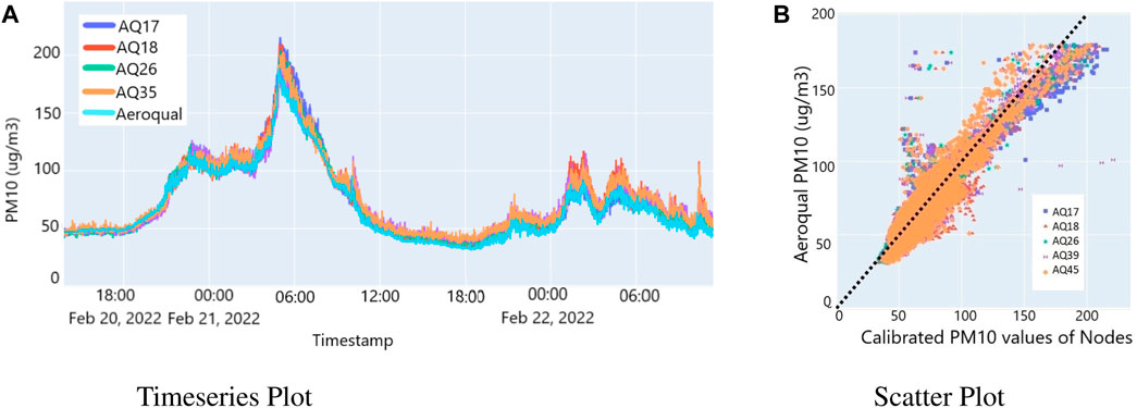
FIGURE 6. Time series and scatter plot of calibrated PM10 data (1-h average). (A) Timeseries Plot, (B) Scatter Plot.

5 Development of web-based dashboard

Figure 7 shows the overview of a web-based dashboard named AirIoT, developed to easily access the real-time data sensed by the deployed sensor devices. AirIoT is a responsive website (https://spcrc.iiit.ac.in/air) that aims to visualize the air pollution levels of the areas where the devices have been deployed. Figure 7A shows the dashboard that provides a view of all the deployed devices and their locations on an interactive map. Figure 7B shows that for all locations, the users can get 10 min average of real-time data and also visualize the trend of the past 48 h. The user can select and deselect the parameters to visualize the trend individually. The dashboard also provides the features of implementing calibration algorithms, authorizing and maintaining user profiles, and logging network activities. Figure 7C shows the basic architecture of the dashboard connecting all the building blocks. The data flow pipe and the sequence of communication steps between the users and the server are presented in Figures 7D, E, respectively.

FIGURE 7

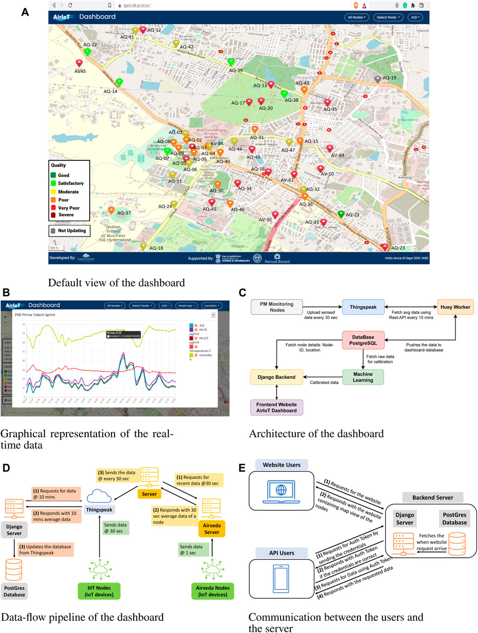
FIGURE 7. Web-based dashboard for real-time air quality data visualization from all deployed devices. (A) Default view of the dashboard, (B) Graphical representation of the real-time data, (C) Architecture of the dashboard, (D) Data-flow pipeline of the dashboard, (E) Communication between the users and the server.

Figure 7C shows the backend of the dashboard, which is built using Django. It is an open-source Python-based framework created using model-template-views architecture. It provides a host of features that efficiently help the data manipulation using GUI. PostgreSQL, an open-source and SQL-compliant relational database management system, is used to store the device’s data on the server (PostgreSQL, 2023). The periodic task of fetching data from the ThingSpeak cloud server to the dashboard is implemented using Huey, a Python queue. Web technologies like CSS, Bootstrap, and Javascript are used to build the dashboard’s front end.

The 43 IIITH devices upload the sensed data on the ThingSpeak server every 30 s, and the 6 Airveda devices upload sensed data on the Airveda server every 1 s. As shown in Figure 7D, all the data from the Airveda server is aggregated at ThingSpeak using a separate REST API with periodic calls for data management on a single platform. The dashboard fetches data from ThingSpeak for all the locations every 10 min and updates the AQI in real-time.

The Django frameworks also help maintain users and their access rights. Figure 7E shows that there are mainly two types of supported users, the website users and the API users. The website users are the system administrators who log in on the admin console to maintain or update network details like adding new devices or updating information like location, sensing parameters, calibration coefficients, etc. On the other hand, the API users are other platforms like mobile applications which can take air quality data from the dashboard to integrate with their services. Every API user must use OAuth authentication to fetch the data from the server. Initially, the API users send their credentials to the server. The server verifies them and responds with a token. This token is used in every request to the API to fetch the server’s data after that.

6 Results and analysis

This section presents mean and variance analysis results and the spatial interpolation for PM10 values in different seasons. Further, the event-driven variation analysis is done for the data collected during the festival of Diwali. It is followed by correlation analysis to understand the range, after which the correlation between the two points is insignificant. Note that the results are shown only in terms of PM10 for brevity, and similar observations have been made for PM2.5 as well.

6.1 Mean and variance

Figure 8 illustrates the mean and variance of PM10 levels during different seasons: monsoon (August 2021), winter (December 2021), and summer (May 2022). The findings indicate that the mean and variance values are highest during winter and lowest during the monsoon season. This pattern aligns with expectations, as the temperature inversion phenomenon in winter, characterized by cold air near the ground and warm air above, tends to trap PM (PM2.5 PM10) near the surface. Conversely, the frequent rainfall during the monsoon helps settle the PM (PM2.5 PM10) particles, reducing their concentration in the air. Figure 8 illustrates the mean and variance of PM10 levels during different seasons: monsoon (August 2021), winter (December 2021), and summer (May 2022). The findings indicate that the mean and variance values are highest during winter and lowest during the monsoon season. Conversely, the frequent rainfall during the monsoon helps settle the PM (PM2.5 PM10) particles, reducing their concentration in the air.

FIGURE 8

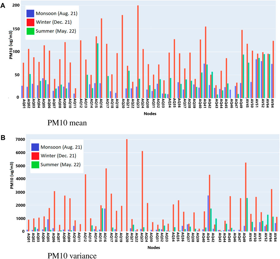
FIGURE 8. Mean and variance of PM10 concentration at the different locations in different seasons. (A) PM10 mean, (B) PM10 variance.

In Figure 8, the three devices with the highest mean PM10 values among the 49 devices are AQ23 (Traffic junction), AQ20 (Green region), and AQ16 (Roadside), while the three devices with the lowest mean PM10 values are AQ11 (Residential area), AQ43 (Roadside), and AQ22 (Roadside). Devices like AQ23 near the traffic junctions have high PM10 exposure due to heavy traffic. Similarly, devices like AQ16 near traffic lights have sluggish traffic flow leading to high mean PM10 concentrations. AQ20 is placed in a high vegetation area but still shows a high mean due to ongoing construction activities in the region. Among the ones with low mean values, AQ11 is placed in a residential area with fewer anthropogenic activities. Similarly, AQ43 and AQ22 are otherwise placed on the roadside but still experience low mean PM10 due to the free flow of traffic and less anthropogenic activities.

These findings highlight the intricate relationship between environmental factors, human activities, and PM10 pollution. They emphasize the need for context-aware monitoring strategies that consider specific locations and associated characteristics to assess air quality at the street level accurately.

6.2 Spatial interpolation

Inverse distance weighting (IDW), one of the most popular spatial interpolation techniques, is used for spatial interpolation in this paper. IDW follows the principle that closer devices will have more impact than farther devices (Longley et al., 2005). A linearly weighted combination of the measured values at the devices is used to estimate the parameters at the nearest location. The weights are a function of the inverse distance between the device’s location and the estimate’s location. Algorithm 1 provides a detailed representation of the IDW algorithm.

Figure 9 shows the IDW-based interpolation maps for PM10 in monsoon (August 21), winter (December 21) and summer (May 22), respectively. For all three seasons, the interpolation results are shown at three different times of the day, 1,100 h, 1,400 h, and 2,100 h, based on hourly averaged PM10 values. Similar to the observations from Figure 8, it can also be observed in these figures that the PM10 concentrations are lowest in monsoon and highest in winter as the frequent rainfall during the monsoon helps settle the PM10 particles and due to temperature inversion phenomenon in winter, PM10 particle trap near the surface.

FIGURE 9

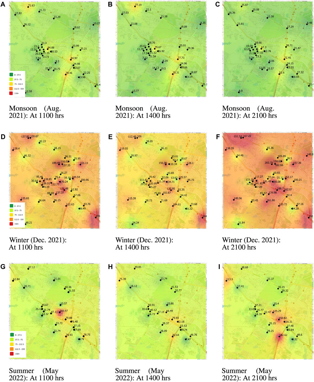
FIGURE 9. Spatial interpolation of PM10 values in three seasons using IDW. (A) Monsoon (August 2021): at 1100 hrs, (B) Monsoon (August 2021): at 1400 hrs, (C) Monsoon (August 2021): at 2100 hrs, (D) Winter (December 2021): at 1100 hrs, (E) Winter (December 2021): at 1400 hrs, (F) Winter (December 2021): at 2100 hrs, (G) Summer (May 2022): at 1100 hrs, (H) Summer (May 2022): at 1400 hrs, (I) Summer (May 2022): at 2100 hrs.

It can be observed from Figure 9 that PM10 concentration was high at 1,100 h and 2,100 h and low at 1,400 h. At 1,100 h, PM10 concentration was high, primarily due to heavy traffic in the area where the device is deployed during office hours. As many office-going people travel to this area during these hours, the density of traffic increases, leading to higher levels of PM10 concentration. As the day progresses, the density of traffic decreases, and the PM10 concentration decreases at 1,400 h. However, with the onset of night, PM10 concentrations can be seen as increased at 2,100 h, falling in peak traffic hours.

The spatial analysis results in this research study offer valuable insights into the spatial distribution of PM10 levels within the study area. Utilizing the IDW interpolation technique, the study successfully estimated PM10 concentrations at unmonitored locations based on the measurements from nearby monitoring devices. The IDW-based interpolation maps showcased the spatial patterns of PM10 concentrations during different seasons and times of the day.

Algorithm 1.Spatial Interpolation Using IDW.

Input: Set of location coordinates of deployed devices X = {x₁, x₂, … , x_n}

Input: Set of PM10 values Y = {y₁, y₂, … , y_n} for the corresponding locations.

Input: Location coordinate of a point of interest c, for which an estimated value will be computed

Output: The interpolated value ${\widehat{y}}_j^{\text{IDW}}$, computed for the location c

Initialization: n ← number of devices deployed

for i = 1 to n do

  d_ij = Euclidean distance between x_i and c_j;

for i = 1 to n do

  $w_{i,j}=\frac{{(d_{i,j})}^{-2}}{{\displaystyle \sum _{k=1}^n}{(d_{k,j})}^{-2}}$;

${\widehat{y}}_j^{\text{IDW}}={\displaystyle \sum _{i=1}^n}(w_{i,j}\cdot y_i)$;return${\widehat{y}}_j^{\text{IDW}}$;

6.3 Event driven variation analysis

Diwali, also known as the festival of lights, is celebrated during the start of the winter. As part of this five-day festival, people burst large numbers of firecrackers in the late evening of the third day of Diwali (4 November 2021). The bursting of firecrackers leads to a significant increase in PM2.5 and PM10 values during those times. Figure 10 shows a time series plot of hourly averaged PM10 values for a few devices over a few days around Diwali. A few critical observations can be made from this figure. First, there was a sudden drop in the PM10 values on the afternoon of 4^th November because of rain. The same has been observed on 5^th and 6^th November afternoons. Second, a clear peak is observed for all the devices during the late evening on 4 November 2021, roughly after 2000 h. For example, the PM10 values in AV64 increased from 40 to 307 before and after bursting crackers. This peak can be attributed to the widespread bursting of firecrackers during the festive celebrations. Third, it can be observed that the PM10 concentrations decrease sharply after a few hours, indicating that the rise was temporary and activity driven.

FIGURE 10

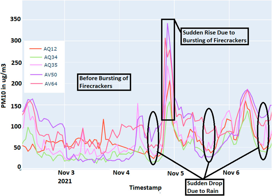
FIGURE 10. Time Series of PM10 (1-Hourly Average) showing the rise in PM10 due to bursting of firecrackers during Diwali.

Further, we see the effect of sparse deployment on the event-driven analysis. Figure 11 shows the IDW-based interpolation maps for PM10 using all 49 devices and sparse deployment of 12 and 4 devices, respectively, at different time instances on 4 November 2021. For sparse deployment, 4 and 12 devices were chosen randomly with the constraint that they should not form a cluster and should also cover different types of regions. It can be seen from Figures 11A–C that the interpolation plot with all 49 devices can identify the event as well as the local hotspots of pollution. Although the interpolation in Figures 11D–F (with 12 devices within 4 km²) can identify the event but is not able to identify the hotspots. On the other hand, the interpolation (with four devices within 4 km²) misses the event entirely and can be misleading. This not only fails to capture the event but also has the potential to yield misleading results. The limited number of devices utilized in this scenario leads to a significant gap in data coverage, resulting in incomplete information about the event.

FIGURE 11

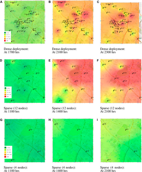
FIGURE 11. A comparison of spatial interpolation of PM10 values during Diwali 2021 for different densities of nodes: Dense deployment (49 nodes), sparse deployment (12 nodes), and sparse deployment (4 nodes). (A) Dense deployment: at 1700 hrs, (B) Dense deployment: at 2100 hrs, (C) Dense deployment: at 2300 hrs, (D) Sparse (12 nodes): at 1100 hrs, (E) Sparse (12 nodes): at 1400 hrs, (F) Sparse (12 nodes): at 1100 hrs, (G) Sparse (4 nodes): at 1100 hrs, (H) Sparse (4 nodes): at 1400 hrs, (I) Sparse (4 nodes): at 2100 hrs.

The root mean square error (RMSE) for different numbers of deployed devices (12 and 4 devices) is calculated. The RMSE for sparse deployments like four devices (59.29) is significantly higher compared to 12 devices (32.47). Consequently, the interpolation algorithm struggles to accurately estimate pollutant levels and identify spatial patterns within the given area. Consequently, relying on this interpolation with a sparse network of devices can lead to erroneous interpretations and misrepresent the actual pollution levels and distribution, potentially leading to misguided decision-making or ineffective mitigation strategies.

The results underscore the significant impact of Diwali celebrations on PM10 concentrations and emphasize the critical role of comprehensive device coverage in conducting precise event-driven analysis. The findings also highlight the limitations of sparse monitoring deployments in effectively capturing localized pollution hotspots. These observations stress the necessity for denser monitoring networks to ensure reliable and accurate air quality assessments during specific events, enabling informed decision-making and effective pollution management strategies.

Algorithm 2.Correlation Coefficient w.r.t Distance.

Input: PM10 sensor values for N nodes: PM10[N]

Input: Location coordinates for N nodes: loc[N]

Output: Coefficients of the exponential model: a, b, c, d

Initialization: Correlation coefficients: tau[ ]

Initialization: Euclidean distances: dist[ ]

for i = 1 to N do

  for j = i + 1 to N do

   ${\text{tau}}_{ij}=\mathtt{c}\mathtt{o}\mathtt{r}\mathtt{r}(PM10[i],PM10[j])$

   ${\text{dist}}_{ij}=\mathtt{e}\mathtt{u}\mathtt{c}\mathtt{l}\mathtt{i}\mathtt{d}\mathtt{i}\mathtt{a}\mathtt{n}(loc[i],loc[j])$   tau ← [tau, tau_ij]   dist ← dist, dist_ij]

Fit Exponential Curve;

 $f=\mathtt{f}\mathtt{i}\mathtt{t}$($dist,tau,{}^{\prime }\mathtt{e}\mathtt{x}\mathtt{p}\mathtt{2}^{\prime })$

 a ← f. a, b ← f. b, c ← f. c, d ← f. d

Return: a, b, c, d

6.4 Correlation analysis

Correlation is a type of bivariate analysis that evaluates the direction and strength of an association between two variables (Boslaugh, 2012). Kendall’s tau method is used as it does not require any presumptions on the data and suits the work in this study. The correlation coefficient’s value ranges from −1 to +1 depending on the strength of the association. Kendall’s correlation coefficients τ between the 49 sensor devices have been calculated using hourly averaged PM10 samples.

A two-term exponential fit is obtained on the correlation values when plotted against the distance between the devices. The fitted model can be written as shown in Eq 4

$f\left(x\right)=a{e}^{bx}+c{e}^{dx},(4)$

where a = 0.4801, b = −0.0124, c = 0.7380 and d = −0.0001 are the coefficients of the best fit for PM10. Algorithm 2 provides a detailed algorithm for finding the correlation coefficient against distance. Figure 12 shows the correlation of PM10 plotted against distance. It can be observed that the change in the correlation coefficient under 350 m is significantly large, after which the decline is gradual. The τ change rate between 0 and 350 m is very fast compared to distances above 350 m. Similar results were obtained for PM2.5 as well. It indicates that the PM monitoring devices shall be deployed at most 350 m apart to capture the spatial variability of PM10 ccurately. Considering the densely populated and rapidly changing nature of Gachibowli, where various land uses such as office spaces, ring roads (highways), residential complexes, and ecological parks are densely packed within a 4 km² area, the observation range of 350 m is justified. This observation range accurately captures the spatial variability of PM10 in such a dynamic environment. This approach ensures that the monitoring network adequately captures the diverse pollution sources and their impacts within Gachibowli’s complex and rapidly evolving landscape. This statistic can help decision-makers determine the optimum density required for effectively monitoring street-level pollution.

FIGURE 12

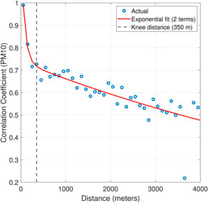
FIGURE 12. Correlation coefficient of PM10 w. r.t distance between the deployed devices to find the optimum distance between two deployment locations.

7 Conclusion

In this paper, an end-to-end low-cost IoT system is developed and densely deployed in Indian urban settings for monitoring PM2.5 and PM10 with fine spatial and temporal resolution. For evaluating the dense deployment, 49 calibrated devices were deployed covering a 4 km² area in Hyderabad, the capital city of Telangana state and the fourth most populated city in India. For data visualization, a web-based dashboard was developed for the real-time interface of PM2.5 and PM10 data. The measurements over the year clearly show a significant difference between the mean and variance of PM2.5 and PM10 values across different locations and seasons. The mean values and the variance were significantly higher in winter than in the summer and the monsoon. The IDW-based spatial interpolation results in monsoon, winter, and summer at three different times show significant spatial variations in PM10 values. Furthermore, variation in PM (PM2.5 and PM10) values before and after the bursting of firecrackers on the day of Diwali is clearly visible in the results. The results also show noticeable temporal variations, with PM10 values rising by 4-5 (AV64) times at the same spot in a few hours, coinciding with Diwali celebrations and identifying the hotspots in dense deployment, which is not noticeable in sparse deployment. It has been shown that the correlation coefficient among a set of devices in the area has low values demonstrating that the PM10 values across a small region may be significantly different. A 350 m distance has been estimated for optimal device deployment for this data set based on insights deduced from the correlation versus distance plot. Thus, there is a need for dense deployment to understand the effect of local pollutants in the air and for improved spatial and temporal resolution of the pollutant data.

The data collected through the established network and the derived insights hold the potential for utilization by relevant authorities and stakeholders in devising and implementing suitable remedies. For instance, city planning authorities can harness the network and data to guide decision-making processes concerning urban planning, infrastructure development, and targeted interventions to mitigate air pollution. An adaptive, non-parametric approach can be implemented to make the data collection robust and energy efficient, allowing the sensing rate to change dynamically based on the maximum frequency estimate derived from recent historical data. Additionally, advanced interpolation techniques, like Kriging, can be explored in future work.

Data availability statement

The raw data supporting the conclusions of this article will be made available by the authors, without undue reservation.

Author contributions

AP: Conceptualization, Data curation, Formal Analysis, Investigation, Methodology, Software, Validation, Visualization, Writing–original draft, Writing–review and editing. SS: Conceptualization, Data curation, Investigation, Software, Visualization, Writing–review and editing. AD: Conceptualization, Methodology, Validation, Writing–original draft, Writing–review and editing. CR: Conceptualization, Methodology, Visualization, Writing–review and editing. IP: Data curation, Methodology, Visualization, Writing–review and editing. SB: Software, Writing–review and editing. SC: Conceptualization, Funding acquisition, Project administration, Resources, Supervision, Validation, Writing–review and editing. KR: Conceptualization, Project administration, Resources, Supervision, Validation, Writing–review and editing. KV: Project administration, Resources, Supervision, Writing–review and editing.

Funding

The author(s) declare financial support was received for the research, authorship, and/or publication of this article. This work is partially supported by the Dept. of Science & Technology (DST), Govt. of India under grant No. 2073 (2020) and Pernod Ricard India Foundation (PRIF) Social Incubator Program 2019, with no conflict of interest.

Acknowledgments

The authors would like to acknowledge the support of Mr Vivek Gupta (Senior Technical Assistant, Electronics Lab, IIITH) and Ritik Yelekar (Intern, SPCRC, IIITH) in the deployment, maintenance and upkeep of all the devices.

Conflict of interest

The authors declare that the research was conducted in the absence of any commercial or financial relationships that could be construed as a potential conflict of interest.

Publisher’s note

All claims expressed in this article are solely those of the authors and do not necessarily represent those of their affiliated organizations, or those of the publisher, the editors and the reviewers. Any product that may be evaluated in this article, or claim that may be made by its manufacturer, is not guaranteed or endorsed by the publisher.

Footnotes

¹Assuming the conversion rate of 1 USD = 83.33 INR in October 2023.

References

Aeroqual (2023). PM10/PM2.5 portable particulate monitor. Available: https://www.aeroqual.com/products/s-series-portable-air-monitors/portable-particulate-monitor#product-overview (Accessed April 8, 2023).

Google Scholar

AeroqualS500 (2023). Aeroqual series 500 – portable air quality monitor. Available: https://www.aeroqual.com/products/s-series-portable-air-monitors/series-500-portable-air-pollution-monitor (Accessed April 8, 2023).

Google Scholar

Airveda (2023). Airveda outdoor air quality monitor. Available: https://www.airveda.com/outdoor-air-quality-monitor (Accessed April 01, 2023).

Google Scholar

Apte, J. S., Messier, K. P., Gani, S., Brauer, M., Kirchstetter, T. W., Lunden, M. M., et al. (2017). High-resolution air pollution mapping with Google street view cars: exploiting big data. Environ. Sci. Technol. 51, 6999–7008. doi:10.1021/acs.est.7b00891

PubMed Abstract | CrossRef Full Text | Google Scholar

Atmo (2023). Atmotube PRO. Available: https://atmotube.com/atmotube-pro (Accessed April 01, 2023).

Google Scholar

Badura, M., Batog, P., Drzeniecka-Osiadacz, A., and Modzel, P. (2018). Evaluation of low-cost sensors for ambient PM2.5 monitoring. J. Sensors 2018, 1–16. doi:10.1155/2018/5096540

CrossRef Full Text | Google Scholar

Becnel, T., Tingey, K., Whitaker, J., Sayahi, T., Lê, K., Goffin, P., et al. (2019). A distributed low-cost pollution monitoring platform. IEEE Internet Things J. 6, 10738–10748. doi:10.1109/JIOT.2019.2941374

CrossRef Full Text | Google Scholar

Borrego, C., Ginja, J., Coutinho, M., Ribeiro, C., Karatzas, K., Sioumis, T., et al. (2018). Assessment of air quality microsensors versus reference methods: the eunetair joint exercise – part II. Atmos. Environ. 193, 127–142. doi:10.1016/j.atmosenv.2018.08.028

CrossRef Full Text | Google Scholar

Boslaugh, S. (2012). Statistics in a nutshell. O’Reilly Media, Inc. Available at: https://www.oreilly.com/library/view/statistics-in-a/9781449361129/

Google Scholar

Brienza, S., Galli, A., Anastasi, G., and Bruschi, P. (2015). A low-cost sensing system for cooperative air quality monitoring in urban areas. Sensors 15, 12242–12259. doi:10.3390/s150612242

PubMed Abstract | CrossRef Full Text | Google Scholar

Census India (2011). Provisional population totals, census of India 2011; cities having population 1 lakh and above. Available: https://censusindia.gov.in/nada/index.php/catalog/1428 (Accessed May 11, 2023).

Google Scholar

Chakraborti, S., Bhatt, S., and Jha, S. (2017). Changing dynamics of urban biophysical composition and its impact on urban heat island intensity and thermal characteristics: the case of Hyderabad City, India. (Accessed 13 April 2023)

Google Scholar

Chen, J., Lu, J., Avise, J. C., DaMassa, J. A., Kleeman, M. J., and Kaduwela, A. P. (2014). Seasonal modeling of pm2.5 in California’s san joaquin valley. Atmos. Environ. 92, 182–190. doi:10.1016/j.atmosenv.2014.04.030

CrossRef Full Text | Google Scholar

Cheng, Y., He, X., Zhou, Z., and Thiele, L. (2019). ICT: in-field calibration transfer for air quality sensor deployments. ACM Interact. Mob. Wearable Ubiquitous Technol. 3, 1–19. doi:10.1145/3314393

CrossRef Full Text | Google Scholar

Clements, A. L., Griswold, W. G., Rs, A., Johnston, J. E., Herting, M. M., Thorson, J., et al. (2017). Low-cost air quality monitoring tools: from research to practice (a workshop summary). Sensors 17, 2478. doi:10.3390/s17112478

PubMed Abstract | CrossRef Full Text | Google Scholar

COMEAP (2010). The mortality Effects of long-term Exposure to particulate air Pollution in the United Kingdom. COMEAP Health Protection Agency Report.

Google Scholar

CPCB India (2015). National air quality index: central pollution control board India (Accessed September 11, 2023).

Google Scholar

Dodge, Y. (2008). The concise encyclopedia of statistics. 1st ed. New York (Accessed April 13, 2023).

Google Scholar

eSIM (2023a). QoSIM UICC assure eSIM specification. Available: https://sensorise.net/products/qosim-m2m-connectivity/qosim/ (Accessed June 18, 2023).

Google Scholar

eSIM (2023b). Sensorise eSIM. Available: https://sensorise.net/tag/esim/.

Google Scholar

Fuller, R., Landrigan, P. J., Balakrishnan, K., Bathan, G., Bose-O'Reilly, S., Brauer, M., et al. (2022). Pollution and health: a progress update. Lancet Planet. Health 6, 535–547. doi:10.1016/s2542-5196(22)00090-0

CrossRef Full Text | Google Scholar

Greenstone, M., Hasenkopf, C., and Lee, K. (2022). Air quality life index. Energy policy institute at the University of Chicago (EPIC).

Google Scholar

Gupta, P., Doraiswamy, P., Levy, R., Pikelnaya, O., Maibach, J., Feenstra, B., et al. (2018). Impact of California fires on local and regional air quality: the role of a low-cost sensor network and satellite observations. GeoHealth 2, 172–181. doi:10.1029/2018GH000136

PubMed Abstract | CrossRef Full Text | Google Scholar

Hernandez, G., Berry, T.-A., Wallis, S., and Poyner, D. (2017). Temperature and humidity effects on particulate matter concentrations in a sub-tropical climate during winter. Int. Proc. Chem., Biol. Environ. Eng. (ICECB). 41–49. doi:10.7763/IPCBEE.2017.V102.10

CrossRef Full Text | Google Scholar

Ihita, G., Viswanadh, K. S., Sudhansh, Y., Chaudhari, S., and Gaur, S. (2021). “Security analysis of large scale IoT network for pollution monitoring in urban India,” in IEEE World Forum on Internet of Things. New Orleans, United States (WF-IoT), 283–288. doi:10.1109/WF-IoT51360.2021.9595688

CrossRef Full Text | Google Scholar

Khot, R., and Chitre, V. (2017). Survey on air pollution monitoring systems. IEEE Int. Conf. Innov. Inf., Embed. Commun. Sys. (ICIIECS), 1–4. doi:10.1109/ICIIECS.2017.8275846

CrossRef Full Text | Google Scholar

Kumar, P., Morawska, L., Martani, C., Biskos, G., Neophytou, M., Di Sabatino, S., et al. (2015). The rise of low-cost sensing for managing air pollution in cities. Environ. Int. 75, 199–205. doi:10.1016/j.envint.2014.11.019

PubMed Abstract | CrossRef Full Text | Google Scholar

Lee, C.-H., Wang, Y.-B., and Yu, H.-L. (2019). An efficient spatiotemporal data calibration approach for the low-cost PM2.5 sensing network: a case study in Taiwan. Environ. Int. 130, 104838. doi:10.1016/j.envint.2019.05.032

PubMed Abstract | CrossRef Full Text | Google Scholar

Lewis, A. C., and Edwards, P. M. (2016). Validate personal air-pollution sensors. Nature 535, 29–31. doi:10.1038/535029a

PubMed Abstract | CrossRef Full Text | Google Scholar

Longley, P. A., Goodchild, M. F., Maguire, D. J., and Rhind, D. W. (2005). Geographic information systems and science. Wiley.

Google Scholar

Lu, Y., Giuliano, G., and Habre, R. (2021). Estimating hourly PM2.5 concentrations at the neighborhood scale using a low-cost air sensor network: A Los Angeles case study. Environ. Res. 195, 110653. doi:10.1016/j.envres.2020.110653

PubMed Abstract | CrossRef Full Text | Google Scholar

Montrucchio, B., Giusto, E., Vakili, M. G., Quer, S., Ferrero, R., and Fornaro, C. (2020). A densely-deployed, high sampling rate, open-source air pollution monitoring WSN. IEEE Trans. Veh. Technol. 69, 15786–15799. doi:10.1109/TVT.2020.3035554

CrossRef Full Text | Google Scholar

Park, H.-S., Kim, R.-E., Park, Y.-M., Hwang, K.-C., Lee, S.-H., Kim, J.-J., et al. (2019). The potential of commercial sensors for short-term spatially dense air quality monitoring: based on multiple short-term evaluations of 30 sensor nodes in urban areas in Korea. Aerosol Air Qual. Res. 20, 369–380. doi:10.4209/aaqr.2019.03.0143

CrossRef Full Text | Google Scholar

Patwardhan, I., Sara, S., and Chaudhari, S. (2021). “Comparative evaluation of new low-cost particulate matter sensors,” in Int. Conf. on Future Internet of Things and Cloud (FiCloud), 192–197.

CrossRef Full Text | Google Scholar

Penza, M., Suriano, D., Pfister, V., Prato, M., and Cassano, G. (2017). Urban air quality monitoring with networked low-cost sensor-systems. Proceedings. doi:10.3390/proceedings1040573

CrossRef Full Text | Google Scholar

Piedrahita, R., Xiang, Y., Masson, N., Ortega, J., Collier, A., Jiang, Y., et al. (2014). The next generation of low-cost personal air quality sensors for quantitative exposure monitoring. Atmos. Meas. Tech. 7, 3325–3336. doi:10.5194/amt-7-3325-2014

CrossRef Full Text | Google Scholar

Popoola, Olalekan, Mead, Mohammed, Stewart, Gregor, Hodgson, T., McLoed, M., Baldoví, José J., et al. (2010). Low-cost sensor units for measuring urban air quality. San Fransisco. AGU Fall Meeting Abstracts.

Google Scholar

PostgreSQL (2023). PostgresSQL object-relational database system. Available: https://www.postgresql.org/about/ (Accessed October 23, 2023).

Google Scholar

Prana (2023). Prana outdoor air quality monitor. Available: https://www.pranaair.com/air-quality-monitor/ambient-air-monitor/ (Accessed April 01, 2023).

Google Scholar

Reddy, C. R., Mukku, T., Dwivedi, A., Rout, A., Chaudhari, S., Vemuri, K., et al. (2020). Improving spatio-temporal understanding of particulate matter using low-cost IoT sensors. IEEE Int. Symp. Pers., Indoor Mob. Radio Commun 1–7. doi:10.1109/PIMRC48278.2020.9217109

CrossRef Full Text | Google Scholar

Robert, E., Burgan, J. C. E., and Hartford, R. A. (1996). Using NDVI to assess departure from average greenness and its relation to fire business. Intermountain Research Station: U.S. Department of Agriculture, Forest Service.

Google Scholar

SDS011 (2023). SDS011 Nova laser PM sensor. Available: http://www.inovafitness.com/en/a/chanpinzhongxin/95.html (Accessed June 18, 2023).

Google Scholar

SHT21 (2023). SHT21 sensirion temperature and humidity sensor. Available: http://www.farnell.com/datasheets/1780639.pdf (Accessed May 18, 2023).

Google Scholar

ThingSpeak (2023). Thingspeak internet of things by MathWorks. Available: https://thingspeak.com/pages/learn_more (Accessed June 05, 2023).

Google Scholar

TTGO (2023). TTGO T-Call ESP32 module Specifications. Available: https://docs.ai-thinker.com/_media/esp32/docs/esp32-sl_specification.pdf (Accessed August 18, 2023).

Google Scholar

Williams, R., Duvall, R., Kilaru, V., Hagler, G., Hassinger, L., Benedict, K., et al. (2019). Deliberating performance targets workshop: potential paths for emerging pm2.5 and o3 air sensor progress. Atmos. Environ. X 2, 100031. doi:10.1016/j.aeaoa.2019.100031

PubMed Abstract | CrossRef Full Text | Google Scholar

Yi, W. Y., Lo, K., Mak, T., Leung, K., Leung, Y., and Meng, M. (2015). A survey of wireless sensor network based air pollution monitoring systems. Sensors 15, 31392–31427. doi:10.3390/s151229859

PubMed Abstract | CrossRef Full Text | Google Scholar

Zhao, C., Wang, Y., Shi, X., Zhang, D., Wang, C., Jiang, J. H., et al. (2019). Estimating the contribution of local primary emissions to particulate pollution using high-density station observations. J. Geophys. Res. Atmos. 124, 1648–1661. doi:10.1029/2018jd028888

CrossRef Full Text | Google Scholar