Distributed rate control of smart solar arrays with batteries

Continued advances in technology have led to falling costs and a dramatic increase in the aggregate amount of solar capacity installed across the world. A drawback of increased solar penetration is the potential for supply-demand mismatches in the grid due to the intermittent nature of solar generation. While energy storage can be used to mask such problems, we argue that there is also a need to explicitly control the rate of solar generation of each solar array in order to achieve high penetration while also handling supply-demand mismatches. To address this issue, we present the notion of smart solar arrays that can actively modulate their solar output based on the notion of proportional fairness. We present a decentralized algorithm based on Lagrangian optimization that enables each smart solar array to make local decisions on its fair share of solar power it can inject into the grid and then present a sense-broadcast-respond protocol to implement our decentralized algorithm into smart solar arrays. We also study the benefits of using energy storage when we rate control solar. To do so, we present a decentralized algorithm to charge and discharge batteries for each smart solar. Our evaluation on a city-scale dataset shows that our approach enables 2.6× more solar penetration while causing smart arrays to reduce their output by as little as 12.4%. By employing an adaptive gradient approach, our decentralized algorithm has 3 to 30× faster convergence. Finally, we demonstrate energy storage can help netmeter more solar energy while ensuring fairness and grid constraints are met.

1 Introduction

The cost of solar energy continues to decline rapidly due to both advances in solar module efficiency and economies of scale in manufacturing. In 2022, the total average cost of energy from solar photovoltaics (PV) worldwide is estimated at 6–8¢ per kilowatt-hour (kWh) (Solar.com, 2023), which is now lower than the average retail electricity rate of 10¢ per kWh (EnergyBot, 2023). Some have predicted that, based on current trends, the marginal cost of solar modules will eventually fall to near zero (Rifkin, 2015). These declining costs, combined with subsidies from various states, are driving significant increases in the number and size of solar deployments. As the cost of solar module hardware decreases, the solar energy cost will be dictated primarily by “balance of system” costs, which capture the indirect costs incurred by utilities to incorporate renewables despite their intermittent nature. These costs include inverters, charge controllers, and energy storage devices, such as batteries, among others.

Conventional wisdom holds that there is a limit to the amount of solar penetration, i.e., the maximum fraction of demand satisfied by solar power that the grid can handle. Since solar generation is intermittent, utilities must offset any large increases or decreases in solar output by decreasing or increasing output from other sources to compensate. However, with high penetration and variable weather conditions, fluctuations in aggregate solar output may occur too quickly to be offset by mechanical generators, resulting in supply-demand mismatches. Consequently, current regulations strictly limit the number and size of grid-connected solar deployments that use net metering.

The problem faced by the grid is reminiscent of problems faced by the early Internet. Early transport protocols for network data transmissions did not include congestion control and allowed users to inject data into the Internet at arbitrarily high rates. Since network capacity was fixed, too many users sending data at excessively high rates drove the network close to congestion collapse. The imminent threat of congestion collapse led to the design of TCP, a transport protocol that uses congestion and rate control to gracefully adapt sending rates upon detecting congestion to maximize aggregate goodput, prevent congestion collapse, and fairly share the Internet’s available bandwidth among active flows (Jacobson and Karels, 1998).

Today’s “dumb” electric grid and solar arrays are akin to the early Internet—it permits grid-tied solar systems to generate and transmit large amounts of power into the grid without regard for its current state and available excess transmission capacity. For example, on a sunny day, the cumulative output of solar deployments throughout the grid could cause a supply-side surplus that exceeds demand and causes grid “congestion”. In contrast, on a cloudy day, the grid may be able to accept additional power from many solar systems that are currently forced off-grid due to strict caps.

To address this problem, we present the notion of smart “active” solar arrays that can intelligently control their solar power output—in contrast to today’s passive solar arrays that simply inject the maximum amount of power they can generate at each instant based on current weather conditions. Smart solar arrays have the ability to accept signals from the grid and can increase or decrease their output (“solar rate”) in response to these signals—similar to TCP, which can modulate its sending rate based on congestion signals. Recent research on software-controlled smart solar inverters (Singh et al., 2017) can be used as a building block for our smart solar arrays. Our contributions are as follows.

1.1 Proportional-share solar rate control

We formulate the problem of solar rate control that allocates the available solar capacity using the notion of proportional fairness. Our approach enables utilities to control the aggregate amount of solar output across its users by setting a limit, or weight, for each array. Each smart array then generates solar power in proportion to its weight. The key challenge for utilities is determining a fair weight for hundreds-to-thousands of deployments in a distributed fashion without continuously gathering fine-grained solar data from each array.

1.2 Decentralized solar rate control algorithm

We present a decentralized algorithm based on Lagrangian optimization that enables each solar array to compute its fair solar rate locally and in a distributed manner using grid signals. We also present a sense-broadcast-respond protocol to implement our decentralized algorithm into smart solar arrays while also enabling fast convergence of our algorithm to the fair rate.

1.3 Battery-based decentralized solar rate control algorithm

We extend the decentralized algorithm to include energy storage. The battery-based decentralized algorithm makes local charge and discharge decisions, independent of other solar arrays. Furthermore, it computes a fair solar rate based on available solar and battery energy, thus, allowing solar arrays to netmeter at a fair rate.

1.4 Implementation and evaluation

We evaluate our approach using a city-scale dataset and show that our distributed rate control algorithm performs similarly to a centralized approach that requires full system knowledge. Our results show that our approach enables 2.6× more solar penetration while causing smart arrays to reduce their output by as little as 12.4%. By employing an adaptive gradient approach, our decentralized algorithm has 3 to 30× faster convergence. Finally, by implementing our decentralized algorithm on a Raspberry Pi-class processor, we demonstrate its feasibility on grid-tied solar inverters with limited processing capabilities. We also evaluate smart solar with batteries and demonstrate that even with a 30-min battery capacity, we can netmeter more solar energy while ensuring fairness and grid capacity constraints are met.

2 Background

2.1 Solar arrays

Solar panels installed on buildings can be connected to the grid through net metering. These grid-tied solar panels support local loads inside a building and feed the surplus power into the grid, effectively selling it back to the utility. However, solar energy generation is intermittent and highly weather dependent (see Figure 1). For example, on sunny days, the amount of solar power generated by a panel is at its maximum, but on overcast days the amount of solar generation may be relatively low. Thus, the amount of solar power “net metered” to the grid depends on: (i) local demand from loads and (ii) the solar radiation incident on the panel, which is weather dependent.

FIGURE 1

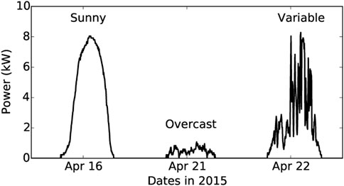
FIGURE 1. Solar power output varies based on time of day and local weather conditions.

Injecting large amounts of solar power is problematic as grid operators must continuously balance supply and demand. If the total output from intermittent solar arrays fluctuates too rapidly, it can cause supply and demand mismatches. Furthermore, as solar penetration grows, the impact of intermittent solar energy makes balancing supply and demand ever more challenging.

To avoid using an “excessive” amount of solar power from being injected into the grid, many governments strictly regulate grid solar connections (50states, 2015). Many states in the US set hard limits by passing laws to regulate the number of solar panel connections. Restricting the solar capacity limits the stochasticity seen from these distributed sources, which in turn makes matching supply and demand a more manageable problem despite intermittency. For example, while the state of Virginia has a cap of 1%, a similar law exists in Massachusetts that caps the solar at 2% of the total power generation. Importantly, these caps are generally based on the rated maximum capacity of a solar installation, regardless of what it actually generates. That is, the caps assume a solar panel is generating at its maximum capacity all the time.

In this paper, we propose an alternate approach—smart solar-powered arrays that are capable of self-regulating their output in a grid-friendly fashion. Our smart solar arrays can control their generation rate by backing off when supply exceeds demand (more precisely, the aggregate solar output is greater than some threshold), and increasing the rate when needed. The idea is similar to rate control of network flows in TCP, where sources back off when there is congestion in the network and increase the rate when the traffic is decreased. While network rate is given by the bandwidth and measured in Mbps, the solar rate is given by the solar power output and measured in kilowatts (kW). We argue that solar rate control has the potential to permit a much larger solar capacity to be installed, thereby increasing solar penetration. Solar rate control also provides grid operators with an additional control “knob” when continuously matching supply and demand.

2.1.1 Relation to energy storage

An alternate solution to managing high solar intermittency is to use energy storage. Energy storage, such as lithium-ion batteries, can absorb surplus energy from solar arrays and feed the excess power back to the grid when there is a deficit (Kanoria et al., 2011; Mishra et al., 2015). Today, the cost of energy storage remains high, and large-scale energy storage deployments remain economically infeasible. However, technology improvements will make energy storage feasible in the future. It is important to note that energy storage and solar rate control are complementary approaches for handling high solar penetration. Both technologies can coexist with one another, and neither obviates the need for the other. For example, even with large scale storage deployments, solar rate control is necessary—since storage batteries, which have finite capacity, may reach full charge and require solar rate control to reduce excess output temporarily. This is similar to “supply-side” demand response, where solar output is temporarily reduced on rare occasion when supply exceeds demand and batteries can not absorb the surplus. Similarly, even with widespread solar rate control deployment, energy storage can be used to locally store excess output that can not be net-metered to the grid. Finally, smart solar arrays also offer a form of “reserve capacity” where their output can be ramped up if there is a sudden increase in demand, a role that energy storage can also play. While energy storage-based techniques have received significant attention in recent years (Qin et al., 2014; Ardakanian et al., 2016; Chau et al., 2016), solar rate control is a newly emerging topic that has not seen much attention and is the focus of this paper. Our work combines both these complementary technologies and understands how energy storage can help when we rate control solar at a city-scale dataset.

2.2 Why is solar rate control feasible?

Interestingly, practically every solar panel today, as well as solar arrays, has the ability to control its output. At an array scale, this can be trivially done in discrete steps by dynamically connecting and disconnecting individual panels. Figure 2A shows an array where panels are connected in parallel and a program switch can be used to dynamically disconnect k out of n panels, thereby providing discrete control¹.

FIGURE 2

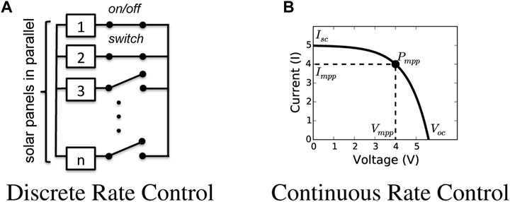
FIGURE 2. Rate control approaches in solar panels. (A) Discrete Rate Control, (B) Continuous Rate Control.

Even at the granularity of a single panel, it is possible to control the output of the panel. The output of photovoltaic solar is given by its I-V curve depicted in Figure 2B. Given a certain amount of solar irradiance, the I-V curve shows all possible operating points of the panel for that solar irradiation. Specifically, any voltage on the curve can be chosen and the panel will then produce the corresponding current. Since power is defined as the product of current and voltage, i.e., P = I ⋅ V, the panel actually can provide a different power output based on the choice of voltage. In general, panels operate at a voltage V at the knee of the curve, which yields the maximum output. The point where the panel generates the maximum power is called the maximum power point (MPP).

However, there is no particular reason to operate a solar panel at its MPP. It is possible to pick other values of V (Hohm and Ropp, 2000; Singh et al., 2017), using a buck-boost converter, which are akin to “backing off” and producing an output less than the output at MPP. Thus, any solar panel’s output can be altered by changing its operating voltage. Our smart solar panels are built on this idea. We assume the presence of software controls that enable the output to be lowered below the maximum power point tracking (MPPT), and thus control the power output of the panel. This mechanism enables continuous rate control to limit the power injected to the grid.

Modern inverters are beginning to offer more configurability, and in the long run, we expect them to expose rate control mechanisms (Singh et al., 2017). Both the discrete control above and the continuous control can be used to regulate the rate. Given smart solar panels connected to the grid, our goal is to control the solar output in order to provide higher control over distributed solar-powered systems.

3 Solar rate control

The problem of controlling solar power is similar to the rate control problem in communication networks (Kelly et al., 1998; Low and Lapsley, 1999). This body of work proposes an optimization framework for determining the rates allocated to different network flows given network capacity constraints. These ideas from network rate control were first applied to the power grid scenario by Ardakanian et al. albeit in a different context—controlling the rate of electric vehicle charging (Ardakanian et al., 2013). In our case, we use these principles from networking (Kelly et al., 1998; Low and Lapsley, 1999) to address the problem of solar rate control. Next, we present the problem of solar rate control. We then outline our design objectives and assumptions.

3.1 Centralized problem

We first formulate our solar rate control problem as a centralized optimization problem. The centralized problem requires knowledge of the load at the feeders/transformers level and the current generation rate of individual solar installations in order to compute the solar allocation rate while adhering to certain grid constraints. The allocation rate should maximize not only the individual user’s output but also the overall grid utilization.

Intuitively, we want to limit the aggregated distributed solar generation to a certain capacity. This leads to the problem of apportioning the capacity among different solar arrays to determine the generation rate for each array. Note that the grid demand and solar generation output are time-varying, and may change over the day. Thus, at each time t, the optimization problem needs to recompute the capacity and the allocation rate for each solar array. For simplicity, we describe the optimization formulation for a single time step.

We consider a distributed grid transmission network with a set of transmission feeders F, transformers K, and smart solar arrays S. Electric power is transmitted from the power station to substations at high voltages. At the distribution substation, i.e., low voltage (LV) feeder, voltage is stepped down and distributed to transformers, wherein it is further stepped down before it is transmitted to residential users. Thus, the smart solar arrays are connected to the LV feeder via a transformer. Formally, we say that the smart solar array s is connected to a LV feeder f, if s ∈ S(k) and f = F(k), where k is the transformer located in between s and f. We model the key characteristics of our problem as follows:

3.1.1 Transformer constraint

Power flow at the transformer level can be bi-directional, and the maximum power flow at the transformer is dependent on the transformer rating $\mathcal{C}$. The transformer rating is between $-\mathcal{C}$ to $\mathcal{C}$ kVA, where the negative sign indicates reverse power flow from the transformers to the feeders. Usually, the transformers are right-sized to ensure that the load at the transformers does not exceed its rating. However, high solar penetration in residential homes may cause reverse power flow and the following constraint must be satisfied to maintain grid stability.

$\sum _s{x}_s\le loa{d}_k+{\mathcal{C}}_k\forall s\in S\left(k\right)\text{\hspace{0.17em}and\hspace{0.17em}}k\in K(1)$

where x_s is the solar generation rate of the smart solar array s ∈ S(k) and load_k is the aggregate load from the residential homes in transformer k.

3.1.2 Feeder constraint

Most residential LV feeders are not equipped with infrastructure to allow reverse power flow, i.e., electricity does not flow from an LV feeder to a medium voltage transmission line and thus obeys the following constraint

$\sum _s{x}_s\le loa{d}_f,\forall s\in S\left(f\right)\text{\hspace{0.17em}and\hspace{0.17em}}f\in F(2)$

where load_f is the load at the feeder f, and S(f) are the smart solar arrays in feeder f.

3.1.3 Grid capacity constraint

The grid utility may cap solar output to reduce variability in the grid or due to legislative reasons (50states, 2015). The aggregate solar generation output may be capped at a fraction of the aggregate grid demand

$\sum _s{x}_s\le capacity,\forall s\in S(3)$

where capacity is defined as a fraction of the total power demand at the grid level.

3.1.4 Solar PV constraint

The maximum power generated by a solar panel lies in the interval $[0,x_s^{\mathit{mppt}}]$, where $x_s^{\mathit{mppt}}$ is the MPPT rate of the solar PV and is defined as

$0\le x_s\le x_s^{\mathit{mppt}}\forall s\in S(4)$

Note that (Eqs 1–3) can be combined and represented as a single inequality

$R\mathbf{x}⪯\mathbf{c}(5)$

where $R\in {\mathbb{R}}^{m\times n}$ matrix, with m combined constraints from (Eqs 1–3) and n smart solar arrays; $\mathbf{x}\in {\mathbb{R}}^{n\times 1}$ vector is the set of smart solar arrays; $\mathbf{c}\in {\mathbb{R}}^{m\times 1}$ vector captures the capacity constraints; and finally, ⪯ represents the generalized inequality of vectors. R can be represented as:

$R_{is}=\left\{\begin{array}{c}1\text{if\hspace{0.17em}}s\in S\text{\hspace{0.17em}is\hspace{0.17em}present\hspace{0.17em}in\hspace{0.17em}the\hspace{0.17em}}{i}^{th}\text{\hspace{0.17em}constraint\hspace{0.17em}}\hfill \\ 0\text{otherwise}\hfill \end{array}\right.$

Remember, our goal is to take some aggregate capacity and apportion it among individual solar installations. Thus, our objective is to maximize the total utility of the individual smart solar arrays U_s(x_s); subject to constraints (Eqs 4, 5). To summarize, our optimization problem can be defined as:

$\begin{array}{lll}\hfill \underset{x_s}{\max }& \sum _{s\in S}{U}_s\left(x_s\right)\hfill & \hfill \\ \hfill \text{subject\hspace{0.17em}to:}& R\mathbf{x}⪯\mathbf{c}\hfill & \hfill \text{and},\\ \hfill & 0\le x_s\le x_s^{\mathit{mppt}}\hfill & \hfill \forall s\in S\end{array}$

We refer to the above problem as the primal problem. We assume that the utility function is strictly concave, increasing, and twice differentiable. Since each constraint is convex, a unique maximizer exists, and solving the optimization problem generates an optimal solar allocation.

The centralized optimization problem discussed earlier is mathematically tractable. However, solving the optimization necessitates a prohibitively high communication overhead, as it requires a two-way communication infrastructure between the smart solar arrays and the control center. Moreover, an increase in solar array deployments will increase the coordination overhead between the control center and smart solar arrays to compute the solar allocation rate. Hence, in Section 4, we formulate a distributed approach that solves the above optimization problem to mitigate some of the issues in the centralized approach.

3.2 Design objectives

3.2.1 Maximize utility to end-users and grid

Solar panels are net-metered and the amount of electricity supplied to the grid earns residential customers billing credits. To model the benefit of net metering, we attribute a utility function U_s(x_s) to the user for generating solar output at rate x_s. From the user’s perspective, each user would like to maximize their own utility. However, from the grid perspective, the utility function should also maximize the overall utilization of the network.

We explore two utility functions, non-weighted and weighted, described in Kelly and Yudovina (2014), which maximizes both the grid and the user’s utility function. The non-weighted utility function, U_s(x_s) = log(x_s), provides equal utility regardless of the size of the solar panel. Since, log(x_s) is a strictly increasing function, an increase in solar output x_s denotes an increase in the utility. On the other hand, the weighted utility, U_s(x_s) = w_s log(x_s), provides additional benefit to users for installing larger solar panel, where weight w_s represents the weight corresponding to the size of the solar panel. Both the utility functions are increasing, strictly concave, and continuously differentiable.

3.2.2 Fairness in solar rate allocation

We are interested in an allocation that is fair to the user. In our paper, we use a utility function that provides proportional fairness and weighted proportional fairness. Any feasible allocation vector x is proportionally fair, if for any other feasible rate vector y, the aggregate of proportional change is non-positive i.e.

$\sum _{s\in S}\frac{y_s-x_s}{x_s}\le 0(6)$

Similarly, any feasible allocation vector x is weighted proportionally fair, if for any other feasible vector y the following holds.

$\sum _{s\in S}{w}_s\frac{y_s-x_s}{x_s}\le 0(7)$

As shown in (Kelly et al., 1998), the logarithmic utility function discussed above achieves proportional fairness, and the allocation vector obeys the fairness property (6). In addition, it is shown that proportional fairness is Pareto optimal, since increasing a user’s allocation will decrease allocation of another user.

3.3 Assumptions

Our proposed approach for rate control of smart solar arrays relies on several key assumptions. First, our approach assumes the availability of a reliable communication infrastructure that facilitates real-time monitoring and control between the control center and the smart solar arrays. This assumption necessitates a communication network with two important characteristics: reliability, ensuring a dependable connection, and low latency to enable timely data exchange. The effectiveness of our approach relies on the availability and performance of this communication link.

We further assume the availability of measurement infrastructure capable of measuring parameters such as current, line voltage, and transformer winding temperature. While these measurement units are typically installed at load buses in the current grid infrastructure, we envision a future scenario where additional measurement nodes will be deployed on load buses, pole transformers, and smart solar arrays.

Furthermore, we assume that these measurement devices are equipped with communication and control modules, enabling them to transmit and receive control signals. This allows for real-time data exchange and coordination between the measurement devices and the central control system.

In terms of the grid structure, our work assumes a radial distribution system, which forms a tree-like structure with load buses interconnected by feeders. In this structure, the load, smart solar arrays, and batteries are typically connected to the leaf nodes of the tree. Additionally, we assume that the batteries are co-located with the smart solar arrays, meaning they are installed at the same location.

Note that we in our grid hierarchy, power flows unidirectionally from the distribution substation to the feeders and below the feeder level, the power flow is bidirectional. However, the unidirectional flow constraint can be easily relaxed by modifying the feeder constraint to include the reverse power constraint. This modification allows for bidirectional power flow within the feeder, accommodating scenarios where power can be injected back into the grid from distributed energy resources.

Additionally, we assume that the solar panels themselves are controllable, allowing for modulation of their power output. This assumption enables us to actively regulate the rate of power generation from the smart solar arrays. Furthermore, we assume that the rate updates at the smart solar arrays are synchronized, meaning that they occur simultaneously. This synchronization is achieved through a broadcast time signal, ensuring that the smart solar arrays operate on the same time frame. While synchronized-based approaches exist, further analysis and exploration of this approach are left for future work.

4 Distributed rate control

The centralized problem discussed in the previous section has three key drawbacks in practice. First, it requires complete knowledge of the maximum generation output (MPP) of all grid-connected smart solar arrays. Second, the control center requires knowledge of the grid’s network topology in order to compute the solar rate. Third, a two-way communication needs to be established between the control center and smart solar arrays to control the solar rate. Hence, we reformulate the centralized optimization problem to an equivalent distributed optimization problem, which can then be solved locally by smart solar arrays and eliminate some of the disadvantages of the centralized approach. In contrast to the centralized approach, the distributed algorithm does not require knowledge of the grid’s network topology and eliminates the need to share local information.

4.1 Dual decomposition

We use the dual decomposition approach to divide the centralized optimization problem into smaller subproblems. Note that the optimization problem has a coupling constraint (5), which prevents solving each subproblem independently. Clearly, without the coupling constraint, each user can maximize its utility independent of the other, thus maximizing the aggregate objective function. Below, we present the Lagrangian dual problem, which relaxes the coupling constraint using control prices (Lagrangian multipliers) and thus allows solving the problem as independent subproblems.

We define the Lagrangian of our optimization problem and consider control prices λ to relax the coupling constraint.

$\mathcal{L}\left(x,\lambda \right)=\sum _{s\in S}{U}_s\left(x_s\right)-\sum _{l\in L}{\lambda }_l\left(y_l-c_l\right)(8)$

$=\sum _{s\in S}\left(U_s\left(x_s\right)-x_s{q}_s\right)+\sum _{l\in L}{\lambda }_l{c}_l(9)$

where l denotes the row number and L is the total number of constraints in matrix R; and.

$y_l=\sum _{s\in S}{R}_{ls}{x}_s\forall l\in L(10)$

$q_s=\sum _{l\in L}{R}_{ls}{\lambda }_l\forall s\in S(11)$

Thus, the Lagrangian dual problem can be formulated as.

$\mathbf{D}\left(\mathit{\lambda }\right):\underset{\lambda \ge 0}{\min }\sum _{s\in S}{V}_s\left(x_s,{\lambda }_s\right)+\sum _{l\in L}{\lambda }_l{c}_l(12)$

$\text{subject\hspace{0.17em}to:}{\lambda }_l\ge 0\forall l\in L(13)$

where,

$V_s\left(x_s,{\lambda }_s\right)=\underset{0\le x_s\le m_s}{\max }\left(U_s\left(x_s\right)-x_s{q}_s\right)\forall s\in S(14)$

As discussed earlier, the utility function (U_s) is strictly concave. Since the sum of the concave function U_s is concave, and the linear constraints are concave, strong duality holds i.e., the primal and the dual solutions are equal. Hence, solving the dual problem solves our original primal problem.

We solve the dual problem using the gradient projection method. Note that for a fixed λ, the dual problem is completely separable in x_s and each subproblem in x_s can be maximized independently by each smart solar array using (14). In particular, for a given price λ, a unique maximizer exists that maximizes (14). Since the utility function U_s is continuously differentiable, using the Karush-Kuhn-Tucker (KKT) theorem², the unique maximum $x_s^{\ast }$ is given by

$x_s^{\ast }=\min \left\{\max \left\{1/U_s^{\prime }\left(x_s\right),0\right\},x_s^{\mathit{mppt}}\right\}(15)$

where $U_s^{\prime }$ is the derivative of the utility function U_s.

The control prices (λ) manage the subproblems and are computed by the master algorithm that solves the dual problem. The master algorithm computes the prices by determining λ that minimizes the objective function in (12). This is done by updating λ using the gradient ∇D(λ) given by

$g_l=\frac{\partial }{\partial {\lambda }_l}D\left(\lambda \right)=c_l-y_l(16)$

The gradient projection algorithm solves the dual problem iteratively. At each iteration, each subproblem is solved parallely, and the master algorithm updates the control prices in opposite direction of the gradient such that

${\lambda }_l\left(t+1\right)=\max \left\{{\lambda }_l\left(t\right)-\gamma \left(c_l-y_l\right),0\right\},\forall l\in L(17)$

where, γ > 0 is an appropriate step size.

4.2 Choosing step size

Our algorithm is similar to the distributed algorithm described in (Ardakanian et al., 2013) and guarantees to converge as ∇D is Lipschitz continuous³ and bounded, provided the step size is appropriately selected. In other words, the convergence of the distributed algorithm is sensitive to the step size used for updating the control prices. While a big step size may cause the algorithm to oscillate around the optimal solution, a small step size may increase the number of iterations required to converge to the solution. Here, we discuss two approaches we used to select a step size to solve the dual problem.

4.2.1 Fixed gradient

At each iteration, the master algorithm updates the control prices using the gradient controlled by a fixed step size parameter using (17). As shown in (Ardakanian et al., 2013), the solution generated by the distributed algorithm converges to the primal-dual optimal when the step size satisfies the following condition

$0<\gamma <2/\bar{\alpha }\bar{L}\bar{S}(18)$

where $\bar{\alpha }={\mathit{max}}_s\{-1/U_s^{″}(x_s)\}$; $\bar{L}={\mathit{max}}_s\{{\sum }_{l\in L}{R}_{ls}\}$ and $\bar{S}={\mathit{max}}_l\{{\sum }_{s\in S}{R}_{ls}\}$.

4.2.2 Adaptive gradient (AdaGrad)

In contrast to the fixed gradient, the adaptive gradient modifies the step size as a function of time and updates the control prices ∀l ∈ L as follows

${\lambda }_l\left(t+1\right)=\max \left\{{\lambda }_l\left(t\right)-\frac{\gamma }{\sqrt{G_l\left(t\right)+ϵ}}\cdot g_l\left(t\right),0\right\}(19)$

where g_l(t) is the gradients w.r.t. λ_l at iteration t; $G_l(t)={\sum }_{i=1}^t{g}_l^2(i)$ is the sum of the squares of g_l up to iteration t; and ϵ = 1e⁻⁸ is a smoothing term to avoid division by zero error. Note that the accumulated sum G_l(t) grows with the number of iterations, which in turn causes the step size to shrink. The benefit of Adagrad is it is not very sensitive to the initial step size, and any appropriate step size converges in reasonable amount of time. The convergence guarantees of Adagrad is well studied and the algorithm converges to the optimal solution (Duchi et al., 2011). Empirically, Adagrad converges faster than the fixed gradient approach and we evaluate both of them in our distributed algorithm.

4.3 System design

Having presented the distributed algorithm that solves our rate control problem, we next describe our assumptions and the Sense-Broadacast-Respond protocol—a round-based protocol. We assume that power flows unidirectionally from the distribution substation to the feeders. However, below the feeder power flow is bi-directional in transformers. Further, we assume the solar arrays have the capability to receive control signals and adjust their rate accordingly.

In our proposed protocol, each round maps to the iterations the distributed algorithm takes to converge to the optimal solution. In each round, prices are computed using (17) and sent to individual smart solar arrays to modulate their power outputs. To better illustrate our Sense-Broadacast-Respond protocol, we describe the steps on how the control center communicates with the smart solar arrays to rate control its power output (see Figure 3).

FIGURE 3

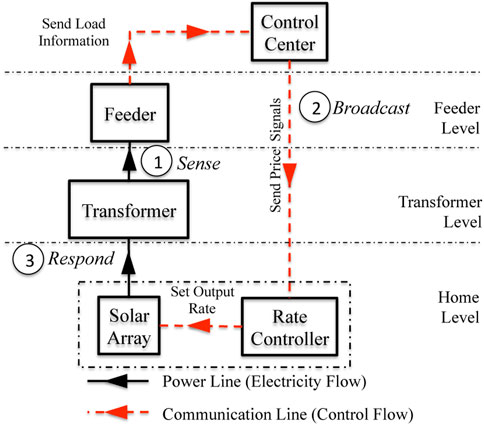
FIGURE 3. Sense–Broadcast–Respond protocol communication among the feeder/transformer level sensors, the control center and the smart solar arrays.

4.3.1 Sense

Sensors at the feeder and transformer capture the load at each time interval. The feeder then communicates the captured information to the grid’s control center using Algorithm 1. Note that the aggregate load sensed at the feeder is the combination of the uncontrolled load from buildings and the regulated power from solar panels and is equivalent to the gradient (c_l − y_l) presented in (16).

Algorithm 1. Feeder/Transformer’s algorithm.

1: while True do

2: sense load_f

3: send load_f information to the control center

4: wait for the next clock tick

5: end

4.3.2 Broadcast

The utility’s control center receives the load from the feeder or transformer and computes the control prices using Algorithm 2. The control prices is adjusted using (17) or (19). Next, the computed control prices are broadcasted to all smart solar arrays.

Algorithm 2. Utility’s control algorithm.

Input: γ

1: while True do

2: receive load from feeders/transformers ∀f, k

3: compute gradient g_l based on the load

4: λ_l \coloneq max{(λ_l − γ∗g_l), 0} ⊳ update control prices

5: broadcast prices to solar s ∈ S(l), in constraint l

6: wait for the next clock tick

7: end

4.3.3 Respond

The smart solar array consists of an identifier pair that associates the array with its parent feeder/transformer. When a smart solar array receives the broadcasted control prices, it computes the rate using (15). The identifier aids in associating the prices relevant to the smart solar array. After the rate is computed, the smart solar array sets its generation rate as shown in Algorithm 3.

Algorithm 3. Smart solar array’s algorithm.

1: while True do

2: receive control price vector λ

3: q_s≔ ∑_l∈LR_lsλ_l ⊳ aggregate price in l

4: $x_s≔{\text{argmax}}_{0\le x_s\le x_s^{\mathit{mppt}}}(U_s(x_s)-x_s{q}_s)$

5: set solar generation rate for x_s

6: wait for the next clock tick

7: end

5 Rate control with battery

The distributed rate control algorithm discussed rate limits individual solar to ensure the aggregate solar output adheres to the grid capacity. Since rate-limiting solar may reduce renewable output, an alternative is to use energy storage to store surplus energy and feed the excess to the grid later.

5.1 Centralized formulation

We begin by formulating the rate control with a battery as a centralized problem. We assume the batteries store any excess energy due to curtailment. Let y_s(t) denote the energy level of the battery at location s at time t. We can model the battery as follows.

$y_s\left(t+1\right)=y_s\left(t\right)+\alpha r_s\left(t\right)-d_s\left(t\right)\forall s,t(20)$

where 0 ≤ α ≤ 1 is the battery efficiency and r_s(t) and d_s(t) are the charge and discharge amounts at location s. The charge and discharge amounts of the battery are upper bounded by $r_s^{\mathit{max}}$ and $d_s^{\mathit{max}}$. Let $y_s^{\mathit{max}}$ denote the maximum capacity of the battery and stored energy is non-negative. Thus, we have:

$0\le y_s\left(t\right)\le y_s^{\mathit{max}}\forall s,t(21)$

Recall that at any time t, we are interested in rate limiting the aggregated distributed solar to a certain capacity. However, if there is energy stored in the battery, it is now possible to netmeter the battery energy to the grid. As shown in Figure 4, we can charge the battery using solar energy and also use the battery to discharge energy. Let z_s(t) denote the total energy netmetered to the grid. Then, the following equality must be satisfied.

$z_s\left(t\right)=x_s\left(t\right)-\alpha r_s\left(t\right)+d_s\left(t\right)\forall s,t(22)$

such that $0\le z_s\le x_s^{\mathit{max}}$ and $x_s^{\mathit{max}}=x_s^{\mathit{mppt}}+\min (d_s^{\mathit{max}},y_s)$.

FIGURE 4

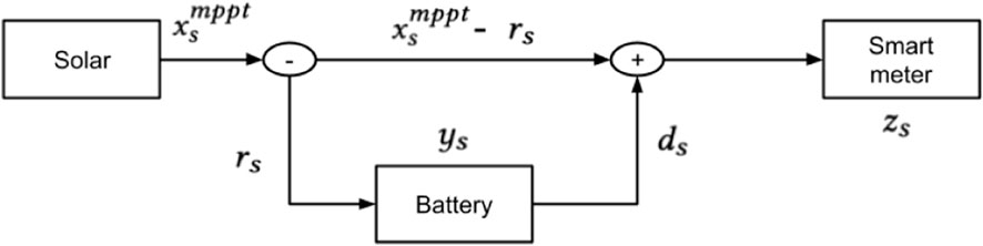
FIGURE 4. Illustrative diagram of rate control with battery.

Lastly, considering the transformer, feeder and grid constraints in (Eqs 1–3), respectively, we have:

$\sum _s{z}_s\left(t\right)\le loa{d}_k\left(t\right)+{\mathcal{C}}_k\forall s\in S\left(k\right)\text{\hspace{0.17em}and\hspace{0.17em}}k\in K(23)$

$\sum _s{z}_s\left(t\right)\le loa{d}_f\left(t\right),\forall s\in S\left(f\right)\text{\hspace{0.17em}and\hspace{0.17em}}f\in F(24)$

$\sum _s{z}_s\left(t\right)\le capacity\left(t\right),\forall s\in S(25)$

Thus, our optimization problem can be defined as:

$\underset{z_s}{\max }\sum _{s\in S}{U}_s\left(z_s\right)$

subject to the constraints in (Eqs 20–25) and (Eq. 4). In comparison to the battery-less scenario, note that each step is dependent on the previous decisions. Because we need to obey the conservation of energy in a battery, the decisions to charge/discharge a battery will affect the state in the following time period. Thus, in the centralized scenario, to find an optimal solution, we need to solve the above optimization for the entire time period. Since this is computationally expensive, we present a decentralized solution of the above centralized solution.

5.2 Battery-based distributed algorithm

We formulate a greedy-based approach, where the decisions can be taken locally at each smart solar array. As before, this approach does not require knowledge of the grid’s network topology or sharing the local generation rate with the grid. The algorithm works as follows. At each time interval t, we first compute the maximum total energy ${\widehat{x}}_s^{\mathit{max}}$ that can be net metered to the grid by smart solar s. Note that we omit the time t for brevity. When the battery is empty, then the maximum energy ${\widehat{x}}_s^{\mathit{max}}$ a solar array can netmeter is equal to $x_s^{\mathit{mppt}}$ value at time t. However, when the battery capacity is nonnegative, we can discharge energy from the battery d_s and netmeter it to the grid, i.e., ${\widehat{x}}_s^{\mathit{max}}=x_s^{\mathit{mppt}}+\min (d_s^{\mathit{max}},y_s(t))$), where $d_s^{\mathit{max}}$ is the max discharge rate, and y_s is the battery capacity at time t.

After we compute the maximum energy that can be net metered, we use the distributed approach in 4 to determine the energy to netmeter to the grid while satisfying grid constraints. Specifically, we use the maximum netmeter energy ${\widehat{x}}_s^{\mathit{max}}$ (instead of $x_s^{\mathit{mppt}}$) and solve the optimization problem in (12) to determine the overall energy to netmeter z_s by each smart solar s. The algorithm determines the netmeter output z_s for each solar s such that it does not exceed the grid capacity. We then use the netmeter output z_s to set the solar generation output x_s as follows.

$x_s=\min \left(z_s,x_s^{\mathit{mppt}}\right)(26)$

The solar generation x_s is set as the minimum of the netmeter output z_s and $x_s^{\mathit{mppt}}$. This is because the solar array can not produce more than the $x_s^{\mathit{mppt}}$ value. Moreover, we use the netmeter output z_s to decide whether to charge or discharge the battery. To determine the charging rate r_s, if the overall netmeter energy z_s is less than the $x_s^{\mathit{mppt}}$, we charge the battery with the excess solar energy as follows.

$r_s=\min \left(x_s^{\mathit{mppt}}-z_s,r_s^{\mathit{max}},y_s^{\mathit{max}}-y_s\right)(27)$

The battery is charged such that the capacity and charging constraints are met. Otherwise, if the overall energy to netmeter z_s is greater than $x_s^{\mathit{mppt}}$, we discharge the battery.

$d_s=\min \left(z_s-x_s^{\mathit{mppt}},d_s^{\mathit{max}},y_s^{\mathit{max}}-y_s\right)(28)$

Finally, the battery state y_s is updated using (20). We outline the algorithm in Algorithm 4.

Theorem 4.1. The greedy-based approach for charging batteries, which selects the maximum available excess energy as its charging rate, with constraint on max charging rate and available storage, at each time step, is an optimal strategy for minimizing solar energy wastage.

Proof. We will prove the optimality of the greedy algorithm using the following two properties:Greedy-choice property: The greedy algorithm makes locally optimal choices at each time step, which leads to a globally optimal solution. Assume there exists an optimal charging strategy that does not agree with the greedy choice at a particular time step t. We omit t for brevity. Let $e=x_s^{\mathit{mppt}}-z_s$ denote the excess solar energy available at time t for smart solar array s. The greedy choice is to charge the battery at the maximum rate possible, $r_s=\min (e,r_s^{\mathit{max}},y_s^{\mathit{max}}-y_s)$.Consider the optimal strategy S_opt, which selects a different charging rate, denoted as r_opt, at time step t. Since S_opt is optimal, we have $r_s^{\mathit{opt}}\le \min (e,r_s^{\mathit{max}},y_s^{\mathit{max}}-y_s)$. By constructing a new charging strategy S_new, which is the same as S_opt except that it adopts the greedy choice of charging rate at time step t, i.e., $r_s=\min (e,r_s^{\mathit{max}},y_s^{\mathit{max}}-y_s)$, we observe that S_new achieves a higher total charge level and potentially lower energy wastage than S_opt. This contradicts the assumption that S_opt is optimal, proving the greedy-choice property.Optimal substructure property: A globally optimal solution can be constructed by combining locally optimal solutions. Let’s assume we have a globally optimal charging strategy S_opt that does not agree with the greedy choice at a particular time step t. We will denote the charging rate chosen by S_opt at time step t as $r_s^{\mathit{opt}}$. Consider the charging strategy S_greedy, which adopts the greedy choice of charging rate at time step t, i.e., r_s. We can construct a new charging strategy S_new, which is the same as S_opt except that it adopts the greedy choice of charging rate at time step t, i.e., r_s. By comparing S_opt and S_new, we can observe the following: (i) For time steps before t, S_opt and S_new are identical. (ii) At time step t, S_new charges the battery at a higher rate than S_opt, as $r_s\ge r_s^{\mathit{opt}}$. (iii) For time steps after t, S_opt and S_new will have the same charging behavior. Since the battery’s charge level at time step t affects the subsequent charging behavior, we can conclude that S_new will have a higher total charge level and potentially lower energy wastage than S_opt. This implies that the globally optimal solution S_opt can be improved by adopting the greedy choice at time step t, leading to S_new with better results. Similarly, we can show that the discharging is optimal as the distributed rate control approach provides an optimal solution for net metering.

Algorithm 4. Smart solar array’s with battery algorithm.

1: while True do

2: $x_s^{\mathit{max}}≔x_s^{\mathit{mppt}}+\min (d_s^{\mathit{max}},y_s)$ ⊳ max netmeter energy

3: receive control price vector λ

4: q_s≔ ∑_l∈LR_lsλ_l ⊳ aggregate price in l

5: $z_s≔{\text{argmax}}_{0\le z_s\le x_s^{\mathit{max}}}(U_s(z_s)-z_s{q}_s)$

6: set solar generation rate for $x_s=\min (z_s,x_s^{\mathit{mppt}})$

7: if $z_s<x_s^{\mathit{mppt}}$ then $r_s=\min (x_s^{\mathit{mppt}}-z_s,r_s^{\mathit{max}},y_s^{\mathit{max}}-y_s)$

8: else $d_s=\min (z_s-x_s^{\mathit{mppt}},d_s^{\mathit{max}},y_s^{\mathit{max}}-y_s)$

9: update battery state y_s

10: wait for the next clock tick

11: end

6 Evaluation

In this section, we describe the dataset and experimental setup for evaluating our distributed algorithm with different utility functions.

6.1 Dataset

For evaluation, we use the smart meter data gathered from a small city in the New England region of the United States. The dataset consists of smart meter data from 11,186 residential homes. Apart from electricity consumption, we also have the electric grid distribution network information—consisting of the feeders-to-transformers-to-meters connections. Table 1 shows a brief description of the dataset characteristics and was obtained from the authors of (Iyengar et al., 2016).

TABLE 1

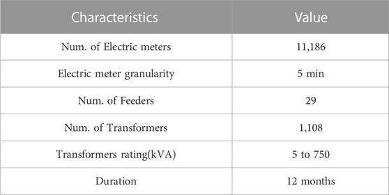
TABLE 1. Key characteristics of the dataset.

The dataset also contains solar power generated from a single residential home. To generate solar power dataset for multiple homes, we first normalize the solar power output using its maximum output for the year. Second, we assume the solar installation sizes to be in the range of 4–10 kW. Next, we scale the normalized solar output with the uniformly generated points for all homes from this range.

6.2 Experimental setup

We run our evaluation for 3 days in the month of April that consists of different solar profiles (see Figure 1) unless otherwise stated. These solar profile patterns are representative of the different fluctuations observed over a year. Along with the solar profiles, we use the load profile from the corresponding dates as an input to our distributed algorithm.

Our distributed approach takes step size γ as an input to the parameter. For the fixed gradient approach, we use $\gamma =2/\bar{\alpha }\bar{L}\bar{S}-ϵ$, as this is the maximum step size to guarantee convergence (18). As discussed earlier, the adaptive gradient (Adagrad) is insensitive to the initial step size. We use γ = 0.5 as the step size for the Adagrad approach. For our experiments, we limit the solar capacity to 15% of the aggregate demand observed at grid level. The time step size is 5 min (granularity of the dataset). In addition, instead of reinitializing the control prices at every time step, we use the control prices of the previous time step as an input for the next time step.

We use the cvxpy library—a python based convex optimization library—to solve the centralized formulation. Internally, the cvxpy solver uses cvxopt solver to find the optimal solution. Separately, for the distributed scenario we use python to simulate the environment.

6.3 Metrics

6.3.1 Fairness metric

To assess the fairness of our algorithms, we use the Gini coefficient to measure the inequality in allocation distribution. The Gini coefficient is a widely used metric in economics to show the distribution (inequality) of income among the residents of a country. The value for the coefficient is between 0 (perfect equality) and 1 (perfect inequality). Mathematically, it is given by (G),

$G=\frac{\sum _{i=1}^n\sum _{j=1}^n\left|x_i-x_j\right|}{2\sum _{i=1}^n\sum _{j=1}^n{x}_j}=\frac{\sum _{i=1}^n\sum _{j=1}^n\left|x_i-x_j\right|}{2\cdot n\sum _{i=1}^n{x}_i}(29)$

where, x_i is the rate allocated to user i and n is the total number of grid-tied solar installations.

6.3.2 Variability metric

Due to solar intermittency, volatility of the load profile observed at the grid level increases with the introduction of solar energy. This increased volatility makes grid operation of matching the demand with supply more challenging, thereby reducing power quality (i.e. more voltage fluctuations). This volatility can be reduced by controlling the solar output. We use variability metric $(\mathcal{V})$ to determine the impact of controlling the rate of solar output and is measured by taking the standard deviation of the successive difference of the power values

$\mathcal{V}=\sigma \left(\mathrm{\Delta }P\right)(30)$

where, P is a vector representing the power generated during the day; ΔP represents the difference between successive values in P; and σ represents the standard deviation function. Higher value indicates more variability. Prior work has used this metric to measure the impact of wind power on increasing variability within the power system Holttinen et al. (2008); we adopt this metric to evaluate the effect of solar rate control in reducing this variability.

6.4 Experimental results

6.4.1 Impact on grid demand

We assume 5% solar penetration at each feeder, i.e. 5% of residential homes have solar panel installations. We compare our approach against no rate control scenario, i.e. each solar panel generates power at its maximum value (MPP).

Figure 5 shows the impact of our distributed rate control on the aggregate grid demand. The aggregate grid demand profiles usually have two peaks—one in the morning and the other in the evening (Figure 5A). The aggregate grid demand with increased solar penetration with no rate control resembles a sitting duck—also known as the duck curve—and causes ramp up and ramp down problems (duc, 2016). Our algorithm ensures that the net demand with solar power converges to the solar cap set by the grid. The solar cap alleviates the ramp down and ramp up problems in power generation due to high solar penetration, thereby reducing the need for expensive peaking power plants. This is clearly seen in Figure 5A, where the ramping up/down need is cut in half.

FIGURE 5

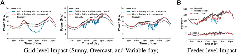
FIGURE 5. Impact of rate control on the aggregate grid demand and feeder-level. With 5% solar penetration and no regulation the solar output exceeds the solar capacity. Our distributed rate control algorithm caps the power output to the desired level. (A) Grid-level Impact (Sunny, Overcast, and Variable day), (B) Feeder-level Impact.

Usually, solar generation on an overcast day is low. Hence, the amount of solar energy generated that exceeds the capacity mandated at the grid level is quite low(Figure 5B). On the other hand, Figure 5C depicts a demand profile with variable solar generation, with generation exceeds the capacity more often and with higher amount than the generation on the overcast day. Our distributed algorithm adjusts the rate such that it does not exceed the solar capacity or the solar array’s maximum generation rate.

We observe a similar behavior at the feeder level (see Figure 5D). Apart from the results shown here, we also ran our simulation for solar penetrations higher than 5%. Even when the maximum solar generation capacity exceeds the local demand, our algorithm limits the rate such that local feeder constraints are met.

Next, we show the impact on variability with and without rate control mechanisms. We compute the variability in the demand curve using (30). We observe that the net demand seen by the grid with rate control is less variable compared to no rate control mechanisms. Table 2 shows the variability metric for three representative solar profiles Figure 5. Note that introduction of solar energy (regulated or unregulated) increases the variability—as shown by the increased values of the variability metric. However, the variability is much lower with rate control than without it. Moreover, with rate control the load profile at the grid level is either less or equally variable compared to no solar scenario.

TABLE 2

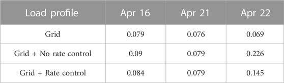
TABLE 2. Variability metric for different days in 2015

Result. Our distributed approach limits the aggregate solar generation output to available solar capacity. Moreover, it decreases the variability in the aggregate grid demand.

6.4.2 Impact of utility function on solar rate

We analyze the behavior of weighted and non-weighted utility functions of our rate control algorithm on different panel sizes. Clearly, at the grid level, the output of both the utility functions remain similar as it maximizes both the grid’s and user’s utility simultaneously. However, the rate allocation generated by the utility functions for individual solar panels would differ based on the size of the solar panel. This is trivially true for the weighted scenario as the allocation is proportional to the size of the panel. In the non-weighted scenario, a smaller sized panel might have reached its maximum generation capacity, thereby allowing larger panels to generate more power. We plot the rate allocation observed on a sunny day for different sized panels (see Figure 6). As expected, in the weighted scenario, we observe each panel backs off its generation rate proportional to the panel size. Whereas, in the non-weighted scenario, each panel generate power at a similar rate (unless its maximum rate is reached).

FIGURE 6

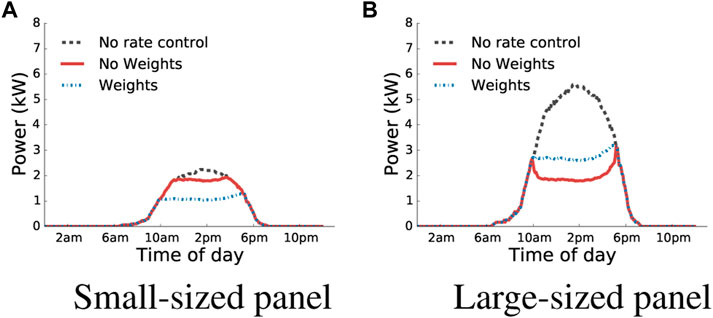
FIGURE 6. Rate allocation for different sized panel. In weighted allocation, each panel backs off its rate proportional to their panel size. However, a non-weighted allocation treats each panel equally and a small-sized panel may generate power equal to a larger sized panel. (A) Small-sized panel, (B) Large-sized panel.

Result. Small sized panels benefit more with non-weighted utility, while weighted utility is favorable to bigger panels.

6.4.3 Impact of solar power control policies

As discussed in Section 1, several states in the US have enforced hard limits on the amount of solar energy net metered into the grid. However, these hard caps are quite conservative and do not exploit the available solar potential. Moreover, these policies limit the adoption of solar by residential homeowners. Here, we analyze the change in the number of homes adopting solar installations and the amount of solar energy generated with different rate control policies. Unlike other experiments, we also assume all panels to be of equal size (5 kW) and evaluate for the entire year 2015. We define the rate control policy as the average hourly curtailment of solar energy per day. For this experiment, we choose rate control policies between 0 and 3 h.

Figure 7A shows the number of homes that can install solar panel systems with different rate curtailment policies. With no daily curtailment, a maximum of 185 homes may be permitted to install solar panels of size 5 kW. However, if we allow just 30 min of average daily curtailment, the number can be increased to 309 homes. As we increase the rate curtailment to an hour, we can double the number of homes adopting solar panel systems. Furthermore, with 2 and 3 h of average daily curtailment we can have 2.6× and 3.4× increase in the number of homes having solar panel systems respectively.

FIGURE 7

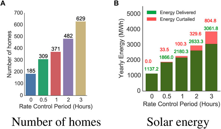
FIGURE 7. Impact of average daily rate control period. (A) Number of homes, (B) Solar energy.

Figure 7B quantifies the amount of energy delivered to and curtailed by the grid with different rate curtailment policies. As discussed earlier, a maximum of 185 homes can install solar panel system when the total installation size is limited to the minimum load observed for the entire year. The total solar energy supplied to the grid from these distributed sources is around 1,137 MWh. However, increasing the average daily curtailment period to 30 min, the solar energy delivered to the grid increases by 64%, with solar energy curtailment of just over 1.8%. Furthermore, increasing the curtailment period to an hour, the installed panels can contribute almost doubles the amount of energy to the grid with solar energy curtailment of 4.6%. Similarly, with 2 and 3 h of average curtailment period, installed solar panels contributes around 2.3× to 2.7× to the grid, with energy curtailment of around 12.5%–26.2% respectively. Clearly, increasing the rate control period increases the solar energy utilization in the grid provided a small fraction of curtailment is allowed. Intuitively, a solar panel only reaches its peak generation capacity around noon on a clear sunny day. For most periods, the power output is a fraction of the total installation size. Thus, increasing the aggregate installation size increases the amount of solar energy utilized by the grid.

Result. Increasing the rate control period, increases the overall solar utilization in the grid. In particular, an average curtailment of 2 h enables 2.6× more solar penetration, while causing smart arrays to reduce their output by as little as 12.4%.

6.4.4 Fairness in solar rate allocation

Our allocation scheme ensures that generation rates of all net-metered solar arrays are assigned in a fair manner—even when solar generation and grid’s capacity vary. We use Gini coefficient, a metric for statistical dispersion, to measure the fairness of our proposed approach.

We compare the two utility functions—weighted and non-weighted—with a solar panel generating power at its maximum capacity (MPP) i. e., no rate control. We evaluate for 3 days with 5% solar penetration at each feeder level (see Figure 8). With no rate control, all panels will generate power at its maximum rate, wherein the rate is proportional to its installation size. Thus, the Gini coefficient is a constant value, that indicates the inequality in the distribution of the panel sizes. Similarly, in the weighted scenario, the rate allocated would be proportional to the size of the panel. Thus, the Gini coefficient does not change with time and is similar to the MPP scenario.

FIGURE 8

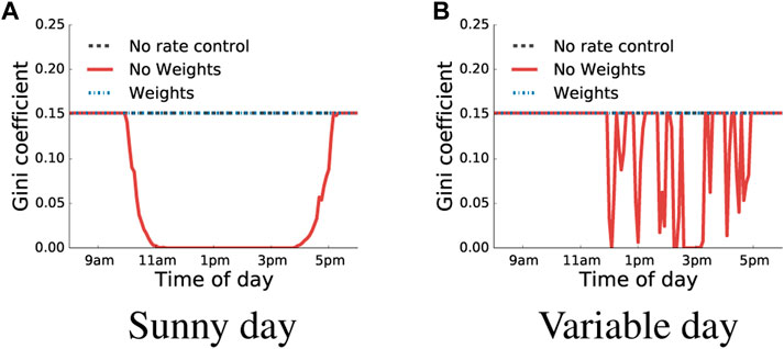
FIGURE 8. Fairness comparison between no rate control mechanism, weighted and non-weighted utility functions. (A) Sunny day, (B) Variable day.

In contrast, the Gini coefficient will not be constant in the non-weighted scenario as depicted in Figure 8. As shown in Figure 8A, until 10 a.m., the Gini coefficient is equivalent to the weighted scenario. This is because even when all the panel generates power at its maximum rate it is not able to meet the total available solar capacity. However, as the day progresses, the total generation exceeds the maximum solar capacity and all the panels are allocated equal rate, which causes the Gini coefficient to reach zero. On an overcast day (not shown in figure), the maximum available capacity is never reached as all the panels operate at MPP. Hence, Gini coefficient is constant. Separately, on a variable day(see Figure 8B), the Gini coefficient varies as it depends on the amount of available capacity met by the generated solar discussed earlier.

Result. Both weighted and non-weighted utilities can be used to achieve fairness in rate allocation.

6.4.5 Convergence of our distributed approach

As discussed earlier, the convergence of the distributed algorithm is dependent on the step size. Theoretically, a large step size will oscillate and not converge to the optimal solution, while a small step size will take a long time to reach the optimal solution. Here, we empirically, compare the performance of two step-size selection methods—i) Fixed gradient, and ii) Adaptive gradient (AdaGrad). We select step sizes and evaluate for all 3 days as described in the experimental setup section. Moreover, we assume that the distributed approach has converged if the objective function’s output is within two consecutive iteration is less than 1e⁻⁵.

Figure 9 shows the convergence results of the distributed algorithm using different step size methods. Note that the distributed algorithm is run for each time instance of a day. The shaded area highlights the range of iteration counts executed by the algorithm to converge over the day. In the fixed gradient method, the mean and the standard deviation of the number of iterations increases linearly with the number of homes with solar panels.

FIGURE 9

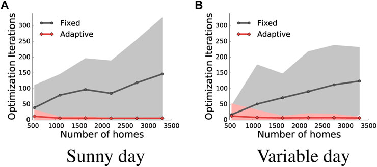
FIGURE 9. Convergence plots of fixed and adaptive gradient using our distributed algorithm. (A) Sunny day, (B) Variable day.

In contrast, the adaptive gradient takes smaller number of iterations—almost 3× to 30× fewer—to converge compared to the fixed gradient approach. Moreover, the adaptive gradient is more reliable, as the standard deviation of the iterations over the day is small. Further, compared to fixed gradient, the number of iterations does not grow linearly in the number of homes with solar panels. However, we notice that on an overcast day, the number of iterations required for both the fixed and the adaptive gradient is almost identical. Due to overcast conditions, the maximum solar generation rate is small, which results in faster convergence.

Result. In comparison to fixed gradient, Adagrad requires 3× to 30× fewer iterations to converge.

6.4.6 Distributed solar rate computation

We assume that a smart solar-powered arrays will have a Raspberry Pi class processor to receive control prices and control its solar rate at every iteration. Thus, we analyze the average time Raspberry Pi takes to complete a single iteration of the distributed algorithm on un-optimized python code. Note that the solar rate computed depends on the size of the control prices which varies based on the size of the distribution network (number of feeders and transformers). However, the number of feeders and transformers change infrequently for a given grid network (once in every few months or years). Thus, the time taken to compute the rate should theoretically remain the same. Figure 10 shows the empirical average time taken to execute the algorithm on Raspberry Pi 3. We observe that the execution time per iteration varies between 2.5 and 3 m. If we assume the average communication time between the control center and the smart solar arrays to be 10 m, with 20 iterations (AdaGrad) per convergence (for 5% solar penetration), the distributed algorithm should take less than 0.3 s to converge.

FIGURE 10

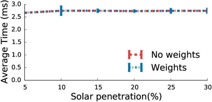
FIGURE 10. Time taken to compute solar rate using control prices in a Raspberry Pi 3.

Result. With 5% penetration, our distributed approach takes less than 0.3 s to find the optimal rate allocation.

6.4.7 Impact of batteries

We analyze the benefits of smart solar with batteries. Note that energy storage mitigates the impact of solar curtailment by storing excess into the battery during the curtailment period. This increases the energy delivered to the grid. We size the battery using the energy consumption pattern of the home. While battery capacity can be expressed in KWh, we use a more intuitive unit, that is, the number of hours a battery can meet the energy demand of a home at its peak. It is equal to the capacity divided by the max discharge rate. Thus, 1× battery size indicates the battery can deliver energy to a home at peak for 1 h.

Figure 11 shows the energy delivered for different battery sizes and different days. As shown, regardless of the day, the energy delivered to the grid increases linearly with an increase in battery size. This indicates that the grid will benefit from local storage even if it is moderately small. In particular, even with 0.5× of battery size, the extra energy delivered is more than 2478 kWh for all days. We also observe that the day type affects the total energy net metered. On a sunny day, doubling the battery size (0.5× to 1×) doubles the energy delivered. However, for a variable or overcast day, increasing the battery size does not increase the energy significantly. This indicates that the location and weather patterns must be considered while sizing the battery for net metering purposes.

FIGURE 11

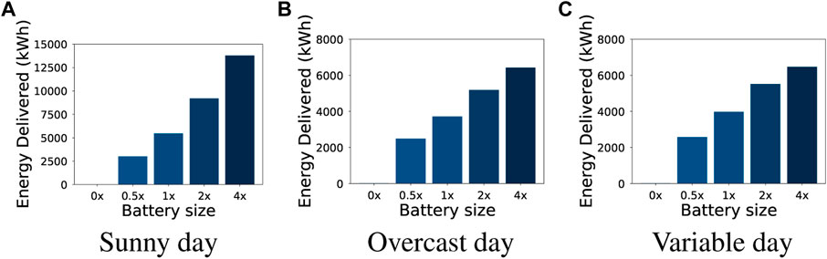
FIGURE 11. Energy delivered to the grid for different days and varying battery sizes. (A) Sunny day, (B) Overcast day, (C) Variable day.

Result. A 30-min battery size on homes with smart solar can reduce the impact of solar curtailment and increase the energy delivered to the grid. However, the location and weather patterns must be considered to determine the ideal battery size.

6.4.8 Impact of charging rate

As before, we assume 5% solar penetration at the feeder level, and homes with solar have a 30-min battery capacity. Further, we assume that the discharge rate is 0.5C; a full-capacity battery can be fully discharged in 2 hours. Figure 12A shows the impact of the rate control with batteries on a variable day. Unlike the no battery scenario, where the solar energy is capped to the capacity, as shown in the figure, the battery is discharged when the maximum rate is below capacity and charged when the battery is above capacity. However, we observe that the max charge/discharge rate limits the amount charged and discharged. Thus, even if the battery has enough capacity to charge and there is sufficient solar, there will be energy wastage because it is limited by the charge/discharge rate.

FIGURE 12

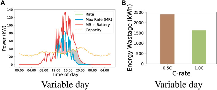
FIGURE 12. (A) Illustrates the charge and discharge pattern of the algorithm on a variable day. As seen, excess solar is charged when the solar power is above the grid capacity (pink shade) and discharges when the solar is below the grid capacity (gray shade) (B) Highlights the impact of different charging rate on energy wastage.

Figure 12B shows the impact of different of battery charging rate. In particular, we observe that a higher charging rate reduces the energy wastage by 32.1%. We note that a higher charging rate (C-rate) shortens battery lifespan(Chen et al., 2018; Xie et al., 2020). However, batteries can support 2C or higher rates and improvements in charging rates will further reduce wastage for curtailment. While we show results for the variable day, sunny days will also benefit from a higher charging rate and reduce energy wastage from curtailment.

Result. Higher battery charging rates reduce solar energy wastage. In particular, increasing the battery charging rate from 0.5C to 1C reduces energy wastage by 32.1%.

6.4.9 Impact of battery on grid demand

Figure 13 illustrates the solar capacity of the grid over time for three distinct days. During the nighttime period when solar generation is absent, the capacity remains at 100%. However, without rate control, there is a possibility of surpassing the solar capacity due to excessive solar generation. In particular, we observe that the capacity can be as low as −300% at midday. In contrast, our approach effectively restricts solar generation to its designated capacity, even when batteries are employed. This stored energy is subsequently discharged when there is lower energy production.

FIGURE 13

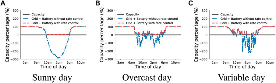
FIGURE 13. Impact of rate control on the aggregate grid demand and feeder-level with batteries. (A) Sunny day, (B) Overcast day, (C) Variable day.

Result. The rate control algorithm has no problem limiting the output from both solar generation and battery to available solar capacity, which also subdues the variability in the grid.

6.4.10 Impact of battery on fairness

Figure 14 shows the impact of battery on fairness. We observe a similar fairness pattern compared to the no battery scenario. With no rate control, the Gini coefficient is zero between 12 a.m. and 6 a.m. because there is no solar generation. However, when solar panels generate power at their maximum rate, the Gini coefficient increases and remains constant, indicating inequality arising from different panel sizes. Interestingly, with batteries, we observe similar fairness in energy generation, where the Gini coefficient is zero between 10 a.m. and 9 p.m. because each solar is equally capped, and as an aggregate, they reach the maximum capacity. However, when smaller batteries are depleted, the inequality rises because larger batteries discharge the remaining stored solar energy to the grid (see Figures14A, B). However, in a weighted scenario, both solar and battery are discharged proportionally to their size and thus, the Gini coefficient remains constant. We note that the increase in the Gini coefficient arises from the ability of larger batteries to discharge more. In particular, we observe such inequality arising when there is not enough solar generation, especially during variable days and at the end of each day.

FIGURE 14

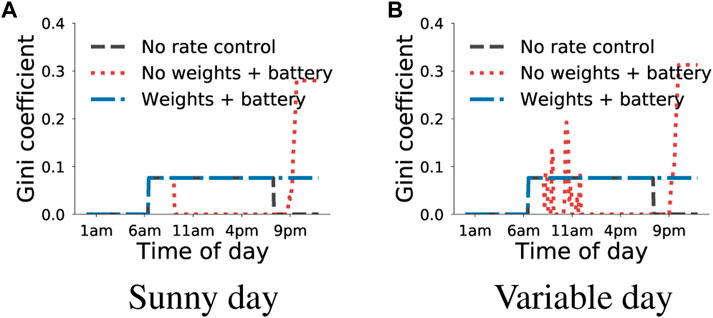
FIGURE 14. Fairness comparison of different utility functions with battery. (A) Sunny day, (B) Variable day.

Result. The algorithm achieves fairness in rate allocation even with batteries.

7 Discussion: Limitations and future work

Our work presents a novel approach to controlling distributed solar with batteries. However, a key limitation is the communication overhead of sending signals to clients. The process of transmitting control signals to the smart solar arrays incurs a certain level of communication overhead. However, it is important to note that a centralized solution would also involve similar overhead and communication delays. Our approach distributes this overhead among the smart solar arrays, which can be more advantageous in terms of scalability and system robustness.

Our work does not specifically investigate the voltage drop problem that may arise in load buses. However, we acknowledge that integrating voltage drop mitigation into our sense-broadcast-control approach is feasible. This can be achieved by monitoring the difference between the line and the rated voltage and utilizing control signals to prevent significant voltage drops. Addressing this voltage drop issue is an important direction for future work.

We utilize batteries to store excess energy and mitigate energy curtailment in our work. However, it is essential to note that batteries have broader applications within smart grid scenarios, including energy cost optimization and grid peak reduction. One potential extension of our work is to analyze the combination of our rate control approach with battery usage in smart grid optimization scenarios. For example, batteries can be used to optimize energy costs by storing energy during low-cost periods and discharging it when electricity prices are higher. This can lead to significant cost savings for consumers and more efficient utilization of renewable energy resources.

Furthermore, batteries can reduce grid peak by absorbing excess power during high-demand periods and supplying it back to the grid when demand surpasses supply. This helps alleviate strain on the grid during peak hours and enhances overall grid stability and reliability. Investigating the integration of battery usage within the context of smart grid optimization, including rate control, is an intriguing avenue for future research. By leveraging the capabilities of batteries in conjunction with rate control algorithms, we can further optimize energy management, improve grid performance, and enhance the overall efficiency of the smart grid system.

8 Related work

A detailed assessment of distributed solar impact on the grid highlights the need for generation flexibility in managing solar variability Bebic (2008). The specific phenomenon of solar over-generation during the day causes large ramp up of power generation through peaking generators, which has been shown to pose operational challenges and put a tremendous amount of stress on the grid duc (2016). Prior work on controlling distributed solar generation include demand side management using storage or load matching Samadi et al. (2016) and solar regulation through curtailment or cutoff. Separately, other research work has focused on distributed generation control Li et al. (2016) and shown distributed and centralized voltage control have similar potential in increasing capacities of distributed generation Vovos et al. (2007).

Numerous studies on solar regulation through curtailment exist Rongali et al. (2016); Lo and Ansari (2012); Tonkoski et al. (2011); Bandyopadhyay et al. (2016). Tonkoski et al. (2011) presents an active power curtailment technique to increase the overall distributed solar capacity at the low-voltage feeder Rongali et al. (2016) describes a voltage-based curtailment where the solar rate is reduced if the sensed voltage is higher than normal. Lo and Ansari (2012) presents a discrete curtailment approach by completely disconnecting the solar units through control signals from the utility’s command center. Recently there have been studies on discrete solar curtailment, where a subset of the solar arrays are disconnected Prasanna et al. (2020); Kuppannagari et al. (2018). In contrast, we present a distributed algorithm that apportions the available solar capacity to individual smart solar arrays through a proportional fairness scheme.

Additionally, machine learning and reinforcement learning have been proposed to help addressing the fairness in solar curtailment among multiple homes Vassallo et al. (2023); Wei et al. (2022); Li et al. (2019); Shahid et al. (2021). Wei et al. (2022) explores the utilization of reinforcement learning to iteratively enhance a fair photovoltaic (PV) curtailment strategy. Vassallo et al. (2023) proposes using reinforcement learning to efficiently and fairly manage voltage control. Li et al. (2019), proposes a deep reinforcement learning (DRL) based algorithm to coordinate multiple PV smart inverters for regulating voltage in the power grid. Similarly, Shahid et al. (2021) introduces a communication-free control scheme using neural networks to mitigate over-voltages in distribution systems with rooftop solar PVs, ensuring fairness and compliance with voltage limits.

In demand-side management, user’s demand and solar generation profile are either scheduled intelligently or shifted using energy storage —- to avoid the risk of excess solar supply. Zhao et al. (2017) presents control algorithms for electric vehicle charging to mitigate the impact of renewable energy integration to the grid. Palensky and Dietrich (2011) discusses different approaches to control demand-side load. Energy storage absorbs excess energy generated from solar and acts as a buffer for large variations in the output Barton and Infield (2004); Denholm et al. (2010); Lee et al. (2021). However, energy storage costs are high, and when energy storage is full, excess solar may still need to be curtailed. Energy storage has also been used to control the ramp rate of solar Sukumar et al. (2018). Since solar output fluctuates, a high ramp rate can introduce significant fluctuations. In our work, we limit solar output fluctuations using the grid capacity parameter and introduce batteries to store the excess energy due to rate control.

Distributed approach for rate control has been widely studied in the networking literature Kelly et al. (1998); Low and Lapsley (1999). However, these approaches are now being studied in the context of rate control of electric vehicles Carvalho et al. (2015); Ardakanian et al. (2013); Rigas et al. (2013). Carvalho et al. (2015) discusses different fairness protocols to mitigate congestion in the grid caused by electric vehicles. Our distributed formulation is similar to the approach proposed in Ardakanian et al. (2013). However, unlike Ardakanian et al. (2013), which explores rate control for electric vehicles—we explore rate control in the context of distributed solar and explicitly model electricity distribution network constraints. Moreover, we extend our decentralized algorithm to incorporate batteries to mitigate the loss of energy from rate control.

9 Conclusion

In this paper, we addressed the problem of growth in solar deployments that could cause supply-demand imbalance due to intermittency in power generation. We designed a decentralized rate control algorithm to allocate generation rate of individual smart solar arrays and apportion the aggregate grid solar capacity through a proportional fairness scheme. Our proposed decentralized algorithm made decisions local to a solar deployment to compute its solar rate without any need for explicit communication with the utility. Furthermore, we designed a battery-based decentralized algorithm that charges the battery during rate control periods and discharges when there is low solar energy production in the grid. We evaluated our rate control algorithm on a city-scale electric distribution network and showed that it generates a fair allocation. We observed that a dynamic rate control achieves significantly higher solar penetration with negligible energy curtailment compared to the current hard caps placed on solar deployments. We also presented convergence results that exhibit the tractability of our algorithm. Finally, our evaluation of solar arrays with batteries demonstrated that having a 30-min battery can further increase solar energy penetration in the grid while satisfying fairness and grid capacity constraints.

Data availability statement

The datasets presented in this article are not readily available because they were obtained from an electric utility company under a non-disclosure agreement. Requests to access the data should be directed to Prashant Shenoy.

Author contributions

PB and SL are the main contributors to the paper and authored the main body of the manuscript. SI contributed towards system design in Section 4 and authored related work and background. PS and DI polished various sections of the manuscript and provided many insightful suggestions. All authors contributed to the article and approved the submitted version.

Funding

This research is supported by NSF grants 1645952, 2020888, 2021693, and 2136199, and the Massachusetts Department of Energy Resources.

Acknowledgments

We thank all the reviewers for their comments and feedback.

Conflict of interest

Author SI was employed by the company Microsoft.

The remaining authors declare that the research was conducted in the absence of any commercial or financial relationships that could be construed as a potential conflict of interest.

Publisher’s note

All claims expressed in this article are solely those of the authors and do not necessarily represent those of their affiliated organizations, or those of the publisher, the editors and the reviewers. Any product that may be evaluated in this article, or claim that may be made by its manufacturer, is not guaranteed or endorsed by the publisher.

Footnotes

¹Typical rooftop solar installation is 5 kW (20 panels). Thus, we can control the power output in 5% (250 W) increments.

²KKT conditions are first order necessary conditions for a nonlinear program to yield a solution that is optimal.

³Lipschitz continuous guarantees existence and uniqueness of a solution.

References

50 states, 201550 states (2015). The 50 states of solar: A quarterly look at America’s fast-evolving distributed solar policy conversation. Available at: https://goo.gl/bXRy3p.

Google Scholar

Ardakanian, O., Keshav, S., and Rosenberg, C. (2016). “Integration of renewable generation and elastic loads into distribution grids,” in SpringerBriefs in electrical and computer engineering.

CrossRef Full Text | Google Scholar

Ardakanian, O., Rosenberg, C., and Keshav, S. (2013). “Distributed control of electric vehicle charging,” in Proceedings of the fourth international conference on Future energy systems.

CrossRef Full Text | Google Scholar

Bandyopadhyay, S., Kumar, P., and Arya, V. (2016). “Planning curtailment of renewable generation in power grids,” in Proccedings of the twenty-sixth international conference on automated planning and scheduling.

CrossRef Full Text | Google Scholar

Barton, J., and Infield, D. (2004). Energy storage and its use with intermittent renewable energy. IEEE Trans. energy Convers. 19, 441–448. doi:10.1109/tec.2003.822305

CrossRef Full Text | Google Scholar

Bebic, J. (2008). Power system planning: Emerging practices suitable for evaluating the impact of high-penetration photovoltaics (NREL).

Google Scholar

California ISO (2016). What the duck curve tells us about managing a green grid. Available at: https://goo.gl/YvI2uc.

Google Scholar

Carvalho, R., Buzna, L., Gibbens, R., and Kelly, F. (2015). Critical behaviour in charging of electric vehicles. New J. Phys. 17, 095001. doi:10.1088/1367-2630/17/9/095001

CrossRef Full Text | Google Scholar

Chau, C. K., Zhang, G., and Chen, M. (2016). Cost minimizing online algorithms for energy storage management with worst-case guarantee. IEEE Trans. Smart Grid 7, 2691–2702. doi:10.1109/tsg.2016.2514412

CrossRef Full Text | Google Scholar

Chen, H., Hu, Z., Zhang, H., and Luo, H. (2018). Coordinated charging and discharging strategies for plug-in electric bus fast charging station with energy storage system. IET Generation, Transm. Distribution 12, 2019–2028. doi:10.1049/iet-gtd.2017.0636

CrossRef Full Text | Google Scholar

Denholm, P., Ela, E., Kirby, B., and Milligan, M. (2010). The role of energy storage with renewable electricity generation

Google Scholar

Duchi, J., Hazan, E., and Singer, Y. (2011). Adaptive subgradient methods for online learning and stochastic optimization. J. Mach. Learn. Res. 12. doi:10.5555/1953048.2021068

CrossRef Full Text | Google Scholar

EnergyBot (2023). Electric rate by state - energybot. Available at: https://www.energybot.com/electricity-rates-by-state.html.

Google Scholar

Hohm, D., and Ropp, M. (2000). “Comparative study of maximum power point tracking algorithms using an experimental, programmable, maximum power point tracking test bed,” in Photovoltaic specialists conference, 2000. Conference record of the twenty-eighth IEEE.

Google Scholar

Holttinen, H., Milligan, M., Kirby, B., Acker, T., Neimane, V., and Molinski, T. (2008). Using standard deviation as a measure of increased operational reserve requirement for wind power. Wind Eng. 32, 355–377. doi:10.1260/0309-524x.32.4.355

CrossRef Full Text | Google Scholar

Iyengar, S., Lee, S., Irwin, D., and Shenoy, P. (2016). “Analyzing energy usage on a city-scale using utility smart meters,” in Proceedings of the ACM international conference on systems for energy efficient build environments.

CrossRef Full Text | Google Scholar

Jacobson, V., and Karels, M. (1998). “Congestion avoidance and control,” in Sigcomm.

Google Scholar

Kanoria, Y., Montanari, A., Tse, S., and Zhang, B. (2011). “Distributed storage for intermittent energy sources: Control design and performance limits,” in 49th annual allerton conference on communication, control, and computing (allerton) (IEEE).

CrossRef Full Text | Google Scholar

Kelly, F., Maulloo, A., and Tan, D. (1998). Rate control for communication networks: Shadow prices, proportional fairness and stability. J. Operational Res. Soc. 49, 237–252. doi:10.1038/sj.jors.2600523

CrossRef Full Text | Google Scholar

Kelly, F., and Yudovina, E. (2014). Stochastic networks, 2. Cambridge University Press.

Google Scholar

Kuppannagari, S. R., Kannan, R., and Prasanna, V. K. (2018). Optimal discrete net-load balancing in smart grids with high pv penetration. ACM Trans. Sens. Netw. (TOSN) 14, 1–30. doi:10.1145/3218583

CrossRef Full Text | Google Scholar

Lee, S., Shenoy, P., Ramamritham, K., and Irwin, D. (2021). Autoshare: Virtual community solar and storage for energy sharing. Energy Inf. 4, 10–24. doi:10.1186/s42162-021-00144-w

CrossRef Full Text | Google Scholar

Li, C., Jin, C., and Sharma, R. (2019). “Coordination of pv smart inverters using deep reinforcement learning for grid voltage regulation,” in 2019 18th IEEE international conference on machine learning and applications (ICMLA) (IEEE), 1930–1937.

CrossRef Full Text | Google Scholar

Li, N., Zhao, C., and Chen, L. (2016). Connecting automatic generation control and economic dispatch from an optimization view. IEEE Trans. Control Netw. Syst. 3, 254–264. doi:10.1109/tcns.2015.2459451

CrossRef Full Text | Google Scholar

Lo, C., and Ansari, N. (2012). Alleviating solar energy congestion in the distribution grid via smart metering communications. IEEE Trans. Parallel Distributed Syst. 23, 1607–1620. doi:10.1109/tpds.2012.125

CrossRef Full Text | Google Scholar

Low, S., and Lapsley, D. (1999). Optimization flow control-I: Basic algorithm and convergence. IEEE/ACM Trans. Netw. 7, 861–874. doi:10.1109/90.811451

CrossRef Full Text | Google Scholar

Mishra, A., Sitaraman, R., Irwin, D., Zhu, T., Shenoy, P., Dalvi, B., et al. (2015). “Integrating energy storage in electricity distribution networks,” in Proceedings of the 2015 ACM sixth international conference on future energy systems.

CrossRef Full Text | Google Scholar

Palensky, P., and Dietrich, D. (2011). Demand side management: Demand response, intelligent energy systems, and smart loads. IEEE Trans. industrial Inf. 7, 381–388. doi:10.1109/tii.2011.2158841

CrossRef Full Text | Google Scholar

Prasanna, V., Kannan, R., Kuppannagari, S., Srivastava, A., Cheung, C. M., Rompokos, A., et al. (2020). DEEP solar: Data DrivEn modeling and analytics for enhanced system layer ImPlementation. Tech. rep. Los Angeles, CA (United States): Univ. of Southern California.

Google Scholar

Qin, J., Chow, Y., Yang, J., and Rajagopal, R. (2014). “Modeling and online control of generalized energy storage networks,” in Proceedings of the 5th international conference on Future energy systems.

CrossRef Full Text | Google Scholar

Rifkin, J. (2015). The rise of the Internet of Things and the race to a zero marginal cost society. Available at: https://goo.gl/smcHB0.

Google Scholar

Rigas, E. S., Ramchurn, S. D., Bassiliades, N., and Koutitas, G. (2013). “Congestion management for urban ev charging systems,” in Smart grid communications (SmartGridComm), 2013 IEEE international conference on (IEEE).

CrossRef Full Text | Google Scholar

Rongali, S., Ganuy, T., Padmanabhan, M., Arya, V., Kalyanaraman, S., and Petra, M. (2016). “iPlug: Decentralised dispatch of distributed generation,” in Comsnets.

CrossRef Full Text | Google Scholar

Samadi, P., Wong, V. W., and Schober, R. (2016). Load scheduling and power trading in systems with high penetration of renewable energy resources.

Google Scholar

Shahid, S., Shafiq, S., Khan, B., Al-Awami, A. T., and Butt, M. O. (2021). A machine learning-based communication-free pv controller for voltage regulation. Sustainability 13, 12208. doi:10.3390/su132112208

CrossRef Full Text | Google Scholar

Singh, A., Lee, S., Irwin, D., and Shenoy, P. (2017). “SunShade: Software-defined solar power,” in Proceedings of the 8th ACM/IEEE international conference on cyber-physical systems.

Google Scholar

Solar.com (2023). Average solar panel cost per kwh in 2023. Available at: https://www.solar.com/learn/solar-panel-cost/.

Google Scholar

Sukumar, S., Mokhlis, H., Mekhilef, S., Karimi, M., and Raza, S. (2018). Ramp-rate control approach based on dynamic smoothing parameter to mitigate solar pv output fluctuations. Int. J. Electr. Power and Energy Syst. 96, 296–305. doi:10.1016/j.ijepes.2017.10.015

CrossRef Full Text | Google Scholar

Tonkoski, R., Lopes, L., and El-Fouly, T. (2011). Coordinated active power curtailment of grid connected pv inverters for overvoltage prevention. IEEE Trans. Sustain. Energy 2, 139–147. doi:10.1109/tste.2010.2098483

CrossRef Full Text | Google Scholar

Vassallo, M., Benzerga, A., Bahmanyar, A., and Ernst, D. (2023). “Fair reinforcement learning algorithm for pv active control in lv distribution networks,” in ICCEP 2023 conference.

Google Scholar

Vovos, P. N., Kiprakis, A. E., Wallace, A. R., and Harrison, G. P. (2007). Centralized and distributed voltage control: Impact on distributed generation penetration. IEEE Trans. Power Syst. 22, 476–483. doi:10.1109/tpwrs.2006.888982

CrossRef Full Text | Google Scholar

Wei, Z., de Nijs, F., Li, J., and Wang, H. (2022). Model-free approach to fair solar pv curtailment using reinforcement learning. arXiv preprint arXiv:2212.06542.

Google Scholar

Xie, W., Liu, X., He, R., Li, Y., Gao, X., Li, X., et al. (2020). Challenges and opportunities toward fast-charging of lithium-ion batteries. J. Energy Storage 32, 101837. doi:10.1016/j.est.2020.101837

CrossRef Full Text | Google Scholar

Zhao, S., Lin, X., and Chen, M. (2017). Robust online algorithms for peak-minimizing ev charging under multistage uncertainty. IEEE Trans. Automatic Control 62, 5739–5754. doi:10.1109/tac.2017.2699290

CrossRef Full Text | Google Scholar