Abstract
Understanding urban spatial heterogeneity of greenhouse gas (GHG) emissions from sectoral household consumption is crucial to facilitate moves towards low-carbon cities. In this study, we use Xiamen city of China as a case study to reveal the emission characteristics of household GHG as well as spatial heterogeneity. We conducted a face-to-face questionnaire survey and calculated GHG emissions of districts from household energy consumption, food consumption, transportation, housing, household waste and wastewater treatment. The GHG emissions and the amount of urban residential household consumption shows obvious spatial heterogeneity across districts. Total GHG emissions of Xiamen city were 8.39 Mt. CO2e, and average household and per capita of GHG emissions were 8.11 and 2.72 tCO2e, respectively. While total GHG emissions vary from 0.41 to 2.45 Mt. CO2e across six districts and range from 0.16 to 3.39 Mt. CO2e among six sectors. Household GHG emissions differ from 7.08 to 9.40 tCO2e, while the per capita emissions range between 2.41 to 3.14 tCO2e among districts. Results also showed that more urbanized areas with higher population density have larger total urban residential GHG emissions, whereas household emissions were comparatively lower in these areas. In contrast, our study did not show an (inverted-) U relationship or linear relationship between emissions and population, nor between emissions and income level. Household energy use is the largest sector emitting GHGs. These findings will be useful to underpin policy making towards low-carbon cities.
Introduction
All countries are facing tremendous pressure to reduce greenhouse gas (GHG) emissions (Wang et al., 2024), with most committing to targets that require reducing the GHG production of high-emitting individuals (Chakravarty et al., 2009; Becken et al., 2024). China ranked first as the largest contributor country for carbon emissions and, at the Paris Climate Conference, China proposed to achieve peak CO2 emissions and to lower carbon emission intensity (CEI) by 60–65% by 2030 (Dong et al., 2018). Urban areas are home to 53% of the Chinese population and its residents produced 75% of national household carbon footprints (HCFs) (Wiedenhofer et al., 2017). Furthermore, cities are projected to experience increasing population concentration (Feng and Hubacek, 2016; Georgescu et al., 2024), and China’s urban population could top 1 billion people in the next two decades (Bai et al., 2014; Sun et al., 2020). Increasing consumption in urbanizing China has been identified as an important driver of household carbon emissions due to the growing urban population and incomes (Peng et al., 2023). Urban household consumption, driven by urbanization and lifestyle changes, has outpaced efficiency improvements in the growth of carbon dioxide (CO2) emissions (Peters et al., 2007; Yan et al., 2023). Cities are taking steps to combat climate change, in spite of the scant progress made by international treaty negotiations (Walmsley et al., 2016). Although methods to account for community-scale emissions have been designed by non-profit organizations—such as the World Business Council for Sustainable Development (WBCSD) and the World Resources Institute (WRI)—most cities lack independent, comprehensive and comparable sources of data (Gurney et al., 2015). For compliance and voluntary policies to be effective, information is needed on the size and composition of household carbon footprints for all regions, at the metropolitan, county, city, and even at the household scales (Jones and Kammen, 2014; Sciara, 2020).
A study conducted by Jones and Kammen (2014) developed econometric models of demand for energy, transportation, food, goods, and services through using United States’ national household surveys data. Those models were used to derive average household carbon footprints (HCF) for United States (US) zip codes, cities, counties, and metropolitan areas. Das Used factor decomposition analysis of India’s household consumption carbon emissions, suggests that increasing population is one of the main reasons for the rise of households’ carbon emissions (Das and Paul, 2014; Koilakou et al., 2024). GHG levels of urban household consumption differ spatially because of households’ lifestyle patterns that vary from place to place. Therefore, treatments and emission reduction plans should be based on spatial heterogeneity especially in the case of rapidly growing cities of China. To do this, it is vital that spatial heterogeneity of GHG is explored, examined and followed. Earlier research has shown that household carbon footprints (HCF) vary considerably: energy, transportation, or consumption is measured using a diverse set of methods which focus largely on large metropolitan cities or regions. Households can vary considerably with households in some locations contributing far more emissions than others (Sovacool and Brown, 2010; Hillman, 2014; Verma et al., 2021).
Most of the previous studies have been limited to analysis of a small set of case studies, especially in case of China, and the resulting conclusions are difficult to generalize beyond the individual studies themselves (Guo et al., 2016; Tong et al., 2016). One of the substantial climate mitigation benefits usually observed is shifting consumer choices, for instance consumption of more vegetarian diets and less red meat, from less to zero fossil-fueled mobility, energy-efficient dwellings, and purchasing high(er)-quality long-lived goods (Girod et al., 2014; Brown et al., 2021; Jack et al., 2021).
While existing research has acknowledged the spatial heterogeneity of urban household consumption GHG emissions, there is a lack of detailed analysis, particularly in rapidly developing cities in China. More in-depth research is needed to understand the differences between various regions and the underlying reasons for these disparities. In addition, most cities currently lack independent, comprehensive, and comparable sources of data on GHG emissions. To formulate effective policies and measures, it is necessary to collect and organize more comprehensive data to accurately assess GHG emissions at various levels, such as cities, counties, communities, and even households. Although it is known that increases in household consumption are an important driver of GHG emissions, there is insufficient quantitative research on the relationship between specific consumption behaviors and GHG emissions. More research is needed to clarify how different consumption patterns impact GHG emissions and to develop targeted emission reduction strategies accordingly.
By addressing these research gaps, the study will contribute to a deeper understanding of urban household consumption-related GHG emissions, enabling the development of more targeted and effective policies and measures to mitigate climate change. Therefore, the primary research questions of this study are: (1) How much heterogeneity exists in different districts? (2) How much of this heterogeneity can be explained by factors—such as development and infrastructure, population density, urbanization level, income, house size—from urban residential consumption in 2015 that are contributing to GHG emissions?
Herein we present the spatial heterogeneity of GHG emissions of urban residential household consumption among six districts and six sectors. Earlier research suggested that scientists should support municipalities to raise awareness of the power of detailed emissions data in tailoring climate and development policies (Walmsley et al., 2016). We quantify the GHG emissions from six districts and six sectors; and consider the cumulative historical development of the six districts. We utilized a detailed questionnaire data of all districts. GHG emissions were analyzed from six sectors including wastewater, solid waste, transportation, food, housing, energy, covering CO2, CH4, N2O. Therefore, the main aim of this research study is to investigate the spatial heterogeneity of GHG emissions of Xiamen city and the socio-environmental attributes such as income and urbanization. Moreover, to identify the associated relationships and to quantify the sectoral greenhouse gas emissions of Xiamen city at the household level to create an inventory.
Materials and methods
Study area
Xiamen, as one of the China’s pilot, low-carbon cities, has committed to explore the ways towards low-carbon transition. Earlier studies (Lin et al., 2015; Guo et al., 2016; Tong et al., 2016) related to emissions of Xiamen city, focused on the whole city or compared it with other cities, yet the development of districts of Xiamen city is extremely heterogenic in terms of economic and social development. In this paper, we identify the spatial heterogeneity and related attributes. Moreover, there is also a lack of published information at the household level considering six districts and six significant sectors of Xiamen city. Therefore, this study used a household survey to collect and analyze such information for Xiamen. For Xiamen city, the urbanization level is nearly 89%, while amongst all the six districts of the city, the urbanization level ranges from 39 to 100%. Per capita income ranges from 23,000 yuan to 51,500 yuan, and the gross domestic product (GDP) of the districts range from 25 billion yuan to 105.7 billion yuan (XMBS, 2016). The uneven development among the districts of Xiamen city demands investigation of spatial heterogeneity of residential household consumption greenhouse gas emissions. In the present study, the spatial heterogeneity of socio-economic factors combined with the GHG emissions in Xiamen city was explored, excluding the natural factors, such as landform, etc. It is important to realize the need to reduce carbon emissions and consider regional inequalities among districts in climate policy.
The selected study area is Xiamen City of Fujian province that consists of six districts. Xiamen is a coastal city in southeastern Fujian province and is one of China’s earliest Special Economic Zones. It lies at 118°04′04″ east longitude and 24°26′46″ north latitude, directly across from the Taiwan Strait, covering an area of the 1699.39 kilometer square (km2). Its resident population increased to 3.86 million in 2015, up from 3.56 million in 2010, with 2.73 people per household (XMBS, 2011, 2016). In the same period, the household area of Xiamen increase to 85.62 km2, and per capita house area to 28.43 meter square (m2), up from 24.19 m2 in 2010 (XMBS, 2011, 2016). Evidence of improved living conditions is seen in the increase in floor area, per capita, of residential housing, which has risen from 3.94 m2 in 1976 to 25.16 m2 in 2012.
In Xiamen city, there are three types of districts according to the urbanization level, population density and GDP, as shown in Supplementary Table S1. Huli and Siming are type I, i.e., completely urbanized with more than 10,000 people/km2 and with a GDP more than 70 million yuan. Jimei and Haicang are type II, where mostly the urbanization level is above 90%, and the population density is between 1,000 and 10,000 people/km2, and with a GDP from 40 to 70 million yuan. Tong’an and Xiang’an are type III, where the urbanization level is below 90%, and the population density is under 1,000 people/km2 and with a GDP below 40 million yuan.
Survey design
Both primary and secondary data were collected. A stratified random sampling technique was used to select 1,150 households in 46 communities, as shown in Supplementary Figure S1. Moreover, the population, number of households, per capita disposable income and GDP of districts and city are taken from the Yearbook of Xiamen Special Economic Zone (2016). Given the heterogeneous spatial demographics of households and residential communities, we applied the spatial sampling method, which takes into account the spatial distribution characteristics of the object, and this method has been used for sampling and statistical inference in the environment, resources, land, ecological, social, and economic sciences. The principle of this method is to balance the cost of sampling with the desired sampling precision, depending on study objectives and spatial variation (Stevens and Olsen, 2004).
Emissions data needs to be merged with socio-economic information—such as income, property ownership or travel habits—and incorporated into software tools that can query policy options and weigh up costs and benefits (Walmsley et al., 2016). The face-to-face questionnaire investigation was established in October 2015, covering the issues of survey household socio-economic information, household energy consumption, household garbage classification, housing and building, transportation and household food consumption. The sample questionnaire consisted of two components: the household socio-economic information and residential consumption. The questionnaire was implemented on a household basis and included household demographics. Survey variables of each component are listed in Supplementary Table S1. After screening 1,150 questionnaires, 1,092 were identified to be valid for analysis.
Accounting methodology
GHGs (including CO2, CH4, N2O) emissions from urban residential consumption focused on six sectors, i.e., energy consumption, transportation, solid waste, wastewater, food, and housing construction material. To quantify GHGs emissions, we followed the guidelines of the Intergovernmental Panel on Climate Change (IPCC), Greenhouse Gas Inventories Research in China, and The Provincial Guidelines for Greenhouse Gas Emission Inventories. Details on the urban residential consumption GHG emissions accounting can be found in the Supplementary material. We used ArcGIS to construct the sample size and distribution in the study area, Supplementary Figure S1. We also used e!Sankey software to show the districts’ emissions from different sectors and sectoral composition, as shown in Figures 1, 2.
Figure 1

Total urban residential household emissions—spatial heterogenic preview. Energy means household energy consumption including the cooling system, heating system, cooking and electricity, the housing including house materials, and its transportation and building house.
Figure 2
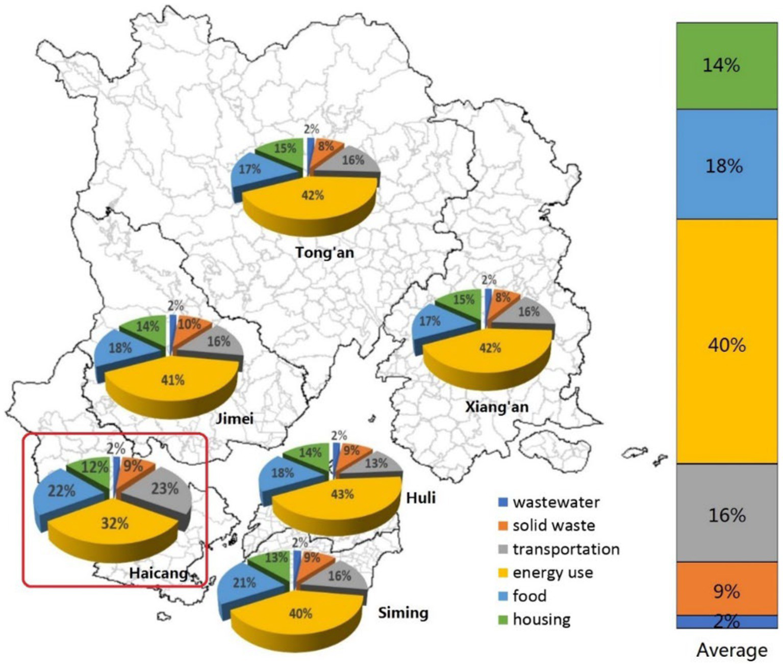
Sectoral contributions of household emissions of Xiamen districts.
Results
GHG emissions from urban residential household consumption
The urban residential GHG emissions of districts and sectors were calculated, as shown in Figure 1. It is important to note that this maps the bottom-up average sample of household emissions to the districts using the numbers of the households in each district. Analyses revealed that the total amount of GHG emissions from urban residential household consumption is 8.39 Mt. CO2e. The total GHG emissions range from 0.16 to 3.39 Mt. CO2e among six sectors, and vary from 0.41 to 2.45 Mt. CO2e among six districts, due to the heterogenic nature and uneven development among the six districts of Xiamen city.
In this study, larger urban residential GHG emissions are found in the more urbanized area with higher population density. Huli was the largest emission district among all six districts, with a total amount of 2.46MtCO2e, followed by Siming with emissions amounting to 2.13Mt CO2e. Jimei was the third largest emission district with the total emissions of 1.48Mt CO2e, followed by Tong’an with the emission level of 0.79 Mt. CO2e. Interestingly, Haicang, with the similar urbanization level and population density to Jimei, emitted 0.77 Mt. CO2e, lower than Tong’an, because of less population. Xiang’an district emitted 0.41 Mt. CO2e, which was the lowest emission district with the lowest urbanization level.
GHG emissions among different sectors
Geographic differences of the total GHG emissions of districts are mainly pronounced for house energy, food, transportation, as shown in Figure 1. Household energy consumption was declared as the largest source of GHG emissions. Generally, the amount of total emissions from the six sectors could be ranked in decreasing order such as: household energy use (3.39 Mt. CO2e) > food (1.52Mt CO2e) > transportation (1.36Mt CO2e) > housing construction material (1.21Mt CO2e) > solid waste (0.75Mt CO2e) > wastewater (0.16Mt CO2e). The proportion of average household emissions of Xiamen city and the districts at sectoral level are shown in Figure 2.
Overall, the emissions from the six sectors, the proportion of six sectors can be ranked in the following decreasing order: household energy use (40%) > food (18%) > transportation (16%) > housing construction material (14%) > solid waste (9%) > wastewater (2%), among the six districts, while the proportion of sectors are different (Figure 2). GHG emissions from household energy use are the largest contributor, representing about 40% proportion, whereas wastewater is the smallest contributing sector among all studied sectors of Xiamen city. Another spatial heterogeneity is found in Haicang and Tong’an districts, which are showing different trends. Transportation and food contributions of Haicang are the highest among the six districts, due to the larger household transportation mileage (especially car) and the largest amount of food consumption. Similarly, household energy usage in Xiang’an is higher than other districts because of larger housing areas compared to the others. This helps explain why Xiang’an has the largest household emissions of the six districts.
At the city scale, emission from house energy use was the largest part, representing about 40% and the proportion of emissions from food, transportation, and house construction materials are similar, representing about 18, 16, 14%, respectively. At the sector scale, the proportion varies from districts and sectors, GHG emissions from household energy use are also the largest, varying from 32% (Haicang) to 43% (Huli). There are big differences among GHG emissions from the transportation sector, which vary from 13% (Huli) to 23% (Haicang). Emissions from food vary from 17% (Xiang’an) to 22% (Haicang). Likewise, the emissions from house construction materials vary from 12% (Haicang) to 15% (Xiang’an); emissions from solid waste range from 8% (Xiang’an and Tong’an) to 10% (Jimei); and emissions from waste water represented about 2% overall.
At the district scale, the composition of household emissions from energy in Haicang (32%) is lower than that in other four districts (40–43%) and city average (40%), due to the small household size. The composition of household emissions from house construction materials in Xiang’an and Tong’an (15%) is higher than that in other districts (12–14%) and city average (14%), due to the larger housing areas. The composition of household emissions from transportation in Haicang (23%) is much higher than that of city average (16%), again this is due to large housing areas, even though the household cars in Haicang is not the highest. The composition of household emissions from food in Siming (21%) and Haicang (22%) is higher than that in other four districts (17–18%), and city average (18%), due to income, household size and average age disparities. The compositions of household emissions from solid waste and wastewater at district scales are not so widely heterogenic.
Household and per capita emissions of districts
Household and per capita average GHG emissions from urban residential consumption of Xiamen city were 8.11 tCO2e and 2.72 tCO2e, respectively. Household GHG emissions vary from 7.08 to 9.40 tCO2e and the per capita emissions ranged between 2.41 to 3.14 tCO2e. The household and per capita GHG emissions of Xiang’an was 9.40 tCO2e and 3.14 tCO2e, respectively, which were the highest of all the six districts as shown in Figure 3. Interestingly, the other five districts were not much higher than the average emissions of the overall city. Siming and Huli districts—both located on the Xiamen Island with 100% urbanization rate—had a household and per capita emissions of 7.08 and 2.41, 7.69 and 2.55 tCO2e, respectively. The household and per capita average GHG emissions from urban residential consumption of Tong’an was 7.75 tCO2e and 2.72 tCO2e, respectively, which was the same as the Xiamen city average. The household GHG emissions from urban residential consumption of Jimei district were 8.37 tCO2e, and its per capita emissions were 2.64 tCO2e, which was 0.12 tCO2e lower than the average of Xiamen city. The household GHG emissions from urban residential consumption of Haicang district were 8.39 tCO2e, and its per capita emissions were 2.84 tCO2e. The highest and lowest districts for the household and per capita average GHG emissions from urban residential consumption were Xiang’an and Siming, respectively. The rankings of the districts according to household emissions and per capita emissions are almost the same: overall, in the six districts, the higher the household emissions, the higher the per capita emissions (except the Jimei district because of high household size).
Figure 3

GHG emissions and income level. Income level 1 = 0–50,000; level 2 = 50,000–100,000; level 2 = 100,000–200,000. Unit: RMB Yuan, yearly.
Discussion
The relationship between emissions and income level
The two key challenges for policymakers are the inequalities of economy, together with environmental degradation (Chancel, 2022; Sinha et al., 2022). A study by Jones and Kammen (2014) concluded that the relationship between HCF and population density suggested an inverted-U relationship, and carbon footprints in the U.S. household tend to be lower at population densities above a threshold of about 3,000 persons per square mile (sqm). In contrast, our study did not show an (inverted-) U relationship or linear relationship between emissions and population, nor between emissions and income level. This may be due to the heterogenic development and history among districts, the evolution of the built-up area, population, urbanization level, GDP, and per capita disposable income.
Accordingly, we defined three types of districts. Among Type I, the correlation between household emissions and household income level was slightly negative where the population density is higher than 10,000 people/km2; in Type II the same correlation tended to be slightly positive with population density between 1,000 to 3,000 people/km2; interestingly, for Type III, where the population density is lower than 1000people/km2, the correlation is clearly negative. In this study, we found that consistently lower household GHG emissions in higher urbanized districts is associated with higher population density, and household income level exhibited a weak though negative correlation with GHG emissions until it exceeds a density threshold (10,000 people/km2), after which the correlation tended to be slightly positive in Type II, while a stronger negative relationship among Type III districts. The population density more than 10,000 persons per km2, the higher the income level, the lower the household and per capita emissions. It was also found that the high-income households emit low emissions among districts where urbanization level is 100%, i.e., a positive correlation existed between household income level and household emissions when the urbanization level is between about 90%; but below 70%, and when it reached 100%, the correlation was negative (Figure 3).
Spatial heterogeneity of household sectoral consumption in Xiamen districts
In this study, we characterized the spatial heterogeneity of urban household GHG emissions from six districts and sectors and revealed the relationships among population density, urbanization level and GHG emissions from urban residential household consumption, and also the relationship between GHG emissions and income level. The spatial heterogeneity of household consumption GHG emissions caused the household consumption patterns, and the household consumption patterns are caused by the geographic differences of development in different districts especially the economy and the infrastructure. Some studies suggest that geographic differences in emissions are partially explained by population density (Sun et al., 2022). Population density affect environmental quality in populous Asian countries (Rahman, 2017; Liu et al., 2023). Population density also displays the largest random-effects variance, which suggests that increasing the residential density would have considerably varied effects across neighborhoods (Xiao et al., 2017; Reisig et al., 2021).
The major differences between sectors of GHG emissions among districts, were energy, food, transportation, and housing. The rapid economic growth and urbanization have resulted in rising energy consumption in Xiamen City, and its total energy consumption reached 10.7696 million tons of coal equivalents (tce), and the energy consumption intensity was 0.569 tce/104 yuan (Lin et al., 2015). We found that the household consumption patterns differed from district to district, shown in Figure 4. It is important to note here that the districts from left side to right side in the abscissa are according to the increasing order of GHG emissions.
Figure 4
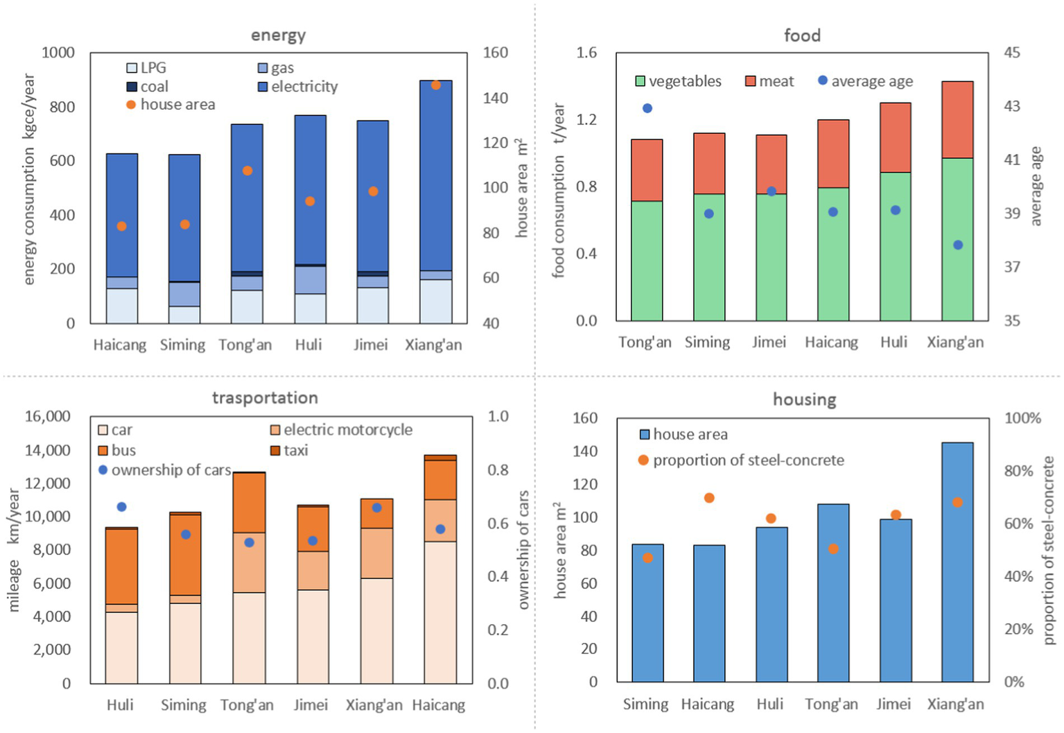
Household sectoral consumption and spatial heterogeneity of Xiamen districts.
For energy consumption, there were four types of energy used by households, electricity consumption was the largest contributor, followed by Liquefied Petroleum gas (LPG), followed by gas, and finally coal. Moreover, the household energy consumption ranged from 622 to 899 kilograms of coal equivalents (kgce) yearly. And the household energy consumption has a high correlation with the housing area, as presented in Supplementary Figure S2 and Figure 4. Households that live in bigger houses potentially consume more energy and emit more GHG emissions. In Xiang’an, household emissions from energy use were highest, because people there live in bigger houses, and such houses demand more energy for heating, cooling, lighting and so on. If people live in a relatively small house, they will consume less energy. Moreover, the energy use structure also affects the GHG emissions. For example, there was higher household total energy consumption in Huli than Jimei, while less GHG emissions, because of less coal and LPG consumption, more gas consumption in Huli than Jimei district. Overall, considering the four types of energy use, Xiang’an was the largest district for household energy consumption, whereas Haicang was the lowest (Figure 4).
For food, the household food consumption varied from 1.08 to 1.43 ton yearly among the six districts. We found a positive relationship between the average age of households of different districts and household GHG emissions due to food consumption (Figure 4). In Xiang’an, household food consumption and GHG emissions from food were the highest among the six districts, while the lowest was observed in Tong’an. We also found that GHG emissions from household food consumption were driven by household income level, as shown in Supplementary Figure S2. Income level has a positive correlation with GHG emissions from food, which means higher income level means potentially higher emissions from food consumption.
For transportation, household mileages ranged from 9,336 to 13,696 km yearly among the six districts. Transport has played a critical role in responding to the challenge of averting dangerous climate change (Razmjoo et al., 2022). The variations of travel carbon emissions within and across neighborhoods highlight the necessity for incorporating population-based heterogeneous GHG emissions distributions into transport governance (Xiao et al., 2017). Huli and Siming, which are in the Xiamen island, have transport mileages that were much lower than other districts out of the Xiamen island. Furthermore, it was found that the mileages of buses were much higher, while the mileages of electric motorcycles were obviously less in the Huli and Siming as compared to other districts. This reflects the better infrastructure and the strict policy of using electric motorcycles in the Xiamen Island. Household mileages of Haicang was highest among the six sectors. Even though household mileages of Tong’an were similar to that of Haicang, the GHG emissions of Tong’an were much lower than the emissions of Haicang. This is due to the higher use of public, rather than private, transport.
For housing, household housing area varied from 84 to 146 m2. In this study, housing emissions were mainly driven by housing area and house structure. For example, houses in Xiang’an are much larger than those in other districts: this is because these people had built their own houses on their own land. Larger houses need more materials and energy result in higher emissions. It is clearly shown in Figure 4; that there are more steel-concrete structure buildings than masonry-concrete buildings in Xiang’an, Haicang and Huli districts. When considering the main difference between sectors, household consumption in Xiang’an was obviously higher than other districts, and in Siming was lowest among the six districts. Household consumption of energy and housing were relatively lower in Haicang, but the consumption of transportation was highest. That was why the household and per capita emissions of Xiang’an were highest, followed by Haicang, and Siming which were lower in emissions. If GHG emissions are to be reduced then the consumption patterns in Xiang’an and Haicang need to be transformed. And household consumption of Siming is relatively lower than another district, even the total amount of GHG emissions are much more than the districts out of the Xiamen Island.
Urban expansion and GHG emission
The consumption patterns in the districts are mainly affected by the development and infrastructure of the districts. Xiamen’s regional GDP reached 347 billion yuan and per capita GDP was 0.09 million yuan, and the ratio of its ‘three-industry structure’1 is 0.7:43.6:55.7 in 2015 (XMBS, 2016). As shown in Figure 5, the Xiamen island, the built-up area is larger and more intensive than the districts out of the Xiamen island. This map shows the basic infrastructure distribution in Xiamen city. It is also evident from Figure 6 that the road connectivity in the island is clearly higher than those out of the island.
Figure 5
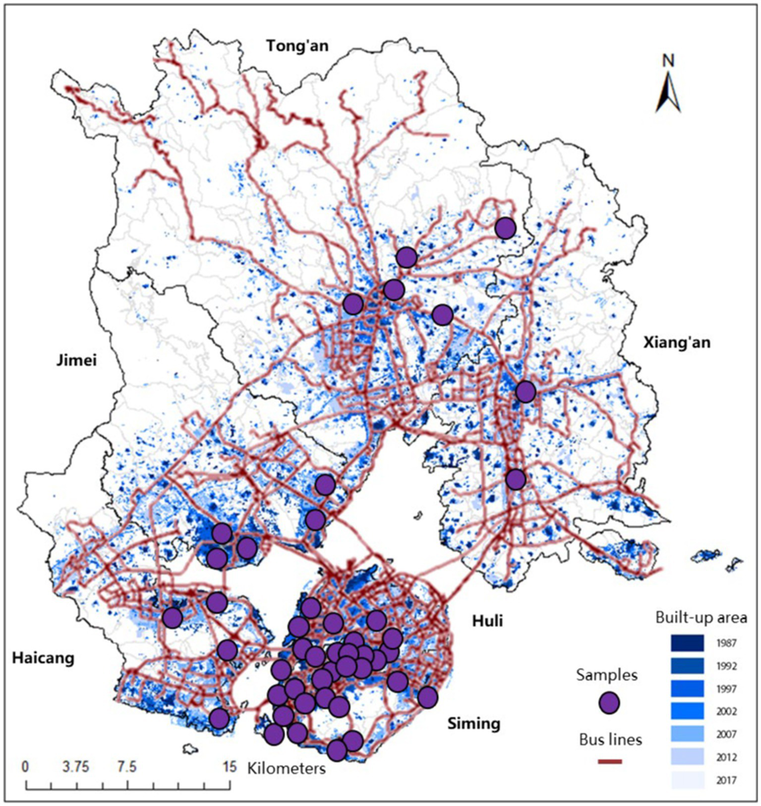
The expansion of the built-up area of Xiamen city.
Figure 6
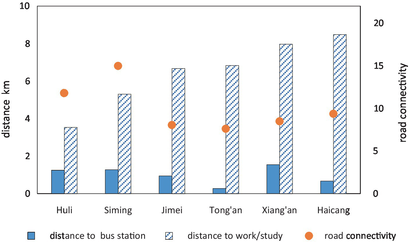
Traffic index of Xiamen city. Road connectivity = number of traffic node/built-up area (km2).
In the most urbanized and high population areas, such as Huli and Siming, people work or study in places closer to home compared to other districts. This helps explain why household transportation mileages in these two districts were lower and GHG from transportation was also lower. Even in these two districts with a greater distance to a bus station, despite better road connectivity it is more convenient for people to take a bus, which helps explain why the household bus mileage here was higher than the other districts. People residing in Haicang relatively travel more for work or study, and the road connectivity here is not as high as in Huli and Siming districts. Thus residents used cars frequently, therefore household total mileage was highest and bus mileage was lower in this district (Figure 6). Private transport does affect the transportation sector and related emissions. Interestingly cars have a positive correlation with transportation. If people living in Jimei, Haicang, Tong’an and Xiang’an use buses instead of cars and motorcycles, household emissions from transportation would be lower. And some measures may make it possible, such as improved road connectivity and increased number of bus stations, means that people are likely to choose to ride buses because of their convenience (Supplementary Figure S2; Figure 6). The households living in neighborhoods without appropriate access to metro stations have higher emissions compared to households with suitable accessibility to metro transport. Shaping a more sustainable city, especially through spatial planning, is argued to have significant potential for GHG mitigation (Carter and Fowler, 2008; Heinonen et al., 2013; Zhang et al., 2021), since the majority of all the global GHG emissions are related to urban areas (Satterthewaite, 2008; Hu et al., 2016; Wei et al., 2021). Higher population density in the urban area may be one potential solution to greenhouse gas emissions, since a higher population density means lower per capita GHG emissions.
Conclusively, Xiang’an is the most district with most potential to emit more GHG, but also has the highest potential to reduce GHG emissions. So far, however, the total amount of GHG emissions in the Xiang’an district are the lowest. Whereas household and per capita emissions in the Xiang’an district are the highest among the six districts. Disparities in the composition, size, and the geographic location of household carbon footprints requires that policies for GHG mitigation are tailored to specific populations.
We propose that densely populated and highly urbanized districts like Siming and Huli should emphasize public transit and energy-efficient construction, whereas Xiang’an and Tong’an may give precedence to renewable energy and sustainable building methods. Moreover, it’s essential to involve the community in mitigation through awareness, education, and participation in decision-making, and to ensure equity by making sustainable choices affordable via incentives, subsidies, or support systems.
Conclusion
Cities are facing challenges of climate change and urbanization, where mitigation deserves an equal priority to reduce the overall adverse effects. However, at the moment, there is a lack of consideration of spatial heterogeneity as one of top priorities in current the policy making of urban greenhouse gas (GHG) emissions reduction. Urban spatial heterogeneity of household GHG emissions and its socio-environmental attributes are considered to be critical elements for urban GHG emissions mitigation. However, there is little understanding of which districts within the city and sectors consumed by households are the most potential mitigation. Moreover, their carbon emission synergies are not well understood.
In this study, we investigate the household GHG emissions in both spatial heterogeneity and socio-environmental attributes. In particular, we quantitatively assess the household GHG emissions from different districts and sectors. Using a coastal city as a case study, we find that GHG emissions and the amount of urban residential household consumption shows obvious spatial heterogeneity across districts. More urbanized areas with higher population density have larger total urban residential GHG emissions, whereas per household emissions were comparatively lower in these areas. Districts exhibit significant heterogeneity in GHG emissions, particularly emissions from household energy use, food, transport and housing. Reducing greenhouse gas emissions from household energy use sectors is a crucial step towards building low-carbon cities and low-carbon households. In recent years, residents’ consumption structure has undergone major changes, and the transformation and upgrading of residents’ consumption structure has a significant impact on carbon emission intensity. It is important for various regions to achieve the goal of “carbon neutrality” by changing residents’ consumption patterns and reducing carbon emission intensity.
Statements
Data availability statement
The original contributions presented in the study are included in the article/Supplementary material, further inquiries can be directed to the corresponding authors.
Author contributions
NY: Writing – original draft, Writing – review & editing, Conceptualization, Data curation, Methodology, Software, Validation, Visualization. LX: Data curation, Investigation, Methodology, Software, Validation, Writing – original draft. GL: Funding acquisition, Project administration, Resources, Supervision, Writing – original draft, Writing – review & editing. SC: Conceptualization, Funding acquisition, Project administration, Resources, Supervision, Writing – review & editing.
Funding
The author(s) declare that financial support was received for the research, authorship, and/or publication of this article. This study is supported by Guangdong Basic and Applied Basic Research Foundation (2023A1515110283), the National Natural Science Foundation of China (No. 52070021) and the Fundamental Research Funds for the Central Universities.
Conflict of interest
The authors declare that the research was conducted in the absence of any commercial or financial relationships that could be construed as a potential conflict of interest.
The author(s) declared that they were an editorial board member of Frontiers, at the time of submission. This had no impact on the peer review process and the final decision.
Publisher’s note
All claims expressed in this article are solely those of the authors and do not necessarily represent those of their affiliated organizations, or those of the publisher, the editors and the reviewers. Any product that may be evaluated in this article, or claim that may be made by its manufacturer, is not guaranteed or endorsed by the publisher.
Supplementary material
The Supplementary material for this article can be found online at: https://www.frontiersin.org/articles/10.3389/frsc.2024.1418214/full#supplementary-material
Footnotes
1.^ The ‘three-industry structure’ is the unit of measurement the Chinese government uses to track economic activity across various sectors. The three industries are primary industry, secondary industry, and tertiary industry. Primary industry includes crop farming, forestry, livestock husbandry and fishery; secondary industry includes industry (including mining and quarrying, manufacturing, electricity, gas and water production and supply industry, etc.) and construction; tertiary industry includes other industries except for the primary and secondary industry, mainly refers to the service sector.
References
1
Bai X. Shi P. Liu Y. (2014). Society: realizing China's urban dream. Nature509, 158–160. doi: 10.1038/509158a
2
Becken S. Miller G. Lee D. S. Mackey B. (2024). The scientific basis of ‘net zero emissions’ and its diverging sociopolitical representation. Sci. Total Environ.918:170725. doi: 10.1016/j.scitotenv.2024.170725
3
Brown M. A. Dwivedi P. Mani S. Matisoff D. Mohan J. E. Mullen J. et al . (2021). A framework for localizing global climate solutions and their carbon reduction potential. Proc. Natl. Acad. Sci.118:e2100008118. doi: 10.1073/pnas.2100008118
4
Carter T. Fowler L. (2008). Establishing green roof infrastructure through environmental policy instruments. Environ. Manag.42, 151–164. doi: 10.1007/s00267-008-9095-5
5
Chakravarty S. Chikkatur A. de Coninck H. Pacala S. Socolow R. Tavoni M. (2009). Sharing global CO2 emission reductions among one billion high emitters. Proc. Natl. Acad. Sci. USA106, 11884–11888. doi: 10.1073/pnas.0905232106
6
Chancel L. (2022). Global carbon inequality over 1990–2019. Nat Sustain5, 931–938. doi: 10.1038/s41893-022-00955-z
7
Das A. Paul S. K. (2014). CO2 emissions fromhousehold consumption in India between 1993–94 and 2006–07: a decomposition analysis. Energy Econ.41, 90–105. doi: 10.1016/j.eneco.2013.10.019
8
Dong F. Long R. Yu B. Wang Y. Li J. Wang Y. et al . (2018). How can China allocate CO2 reduction targets at the provincial level considering both equity and efficiency evidence from its Copenhagen accord pledge. Res Conserv Recycl130, 31–43. doi: 10.1016/j.resconrec.2017.11.011
9
Feng K. Hubacek K. (2016). Carbon implications of China’s urbanization. Energy Ecol. Environ.1, 39–44. doi: 10.1007/s40974-016-0015-x
10
Georgescu M. Broadbent A. M. Krayenhoff E. S. (2024). Quantifying the decrease in heat exposure through adaptation and mitigation in twenty-first-century US cities. Nature Cities1, 42–50. doi: 10.1038/s44284-023-00001-9
11
Girod B. van Vuuren D. P. Hertwich E. G. (2014). Climate policy through changing consumption choices: options and obstacles for reducing greenhouse gas emissions. Glob. Environ. Chang.25, 5–15. doi: 10.1016/j.gloenvcha.2014.01.004
12
Guo F. Kurdgelashvili L. Bengtsson M. Akenji L. (2016). Analysis of achievable residential energy-saving potential and its implications for effective policy interventions: a study of Xiamen city in southern China. Renew. Sust. Energ. Rev.62, 507–520. doi: 10.1016/j.rser.2016.04.070
13
Gurney K. R. Romero-Lankao P. Seto K. C. Hutyra L. R. Duren R. Kennedy C. et al . (2015). Track urban carbon emissions on a human scale. Nature525, 179–181. doi: 10.1038/525179a
14
Heinonen J. Jalas M. Juntunen J. K. Ala-Mantila S. Junnila S. (2013). Situated lifestyles: I. How lifestyles change along with the level of urbanization and what the greenhouse gas implications are—a study of Finland. Environ. Res. Lett.8:025003. doi: 10.1088/1748-9326/8/2/025003
15
Hillman T. R. A. (2014). Greenhouse gas emission footprints and energy use benchmarks for eight U.S. Cites. Environ. Sci. Technol44, 1902–1910. doi: 10.1021/es9024194
16
Hu Y. Lin J. Cui S. Khanna N. Z. (2016). Measuring urban carbon footprint from carbon flows in the global supply chain. Environ. Sci. Technol.50, 6154–6163. doi: 10.1021/acs.est.6b00985
17
Jack M. W. Mirfin A. Anderson B. (2021). The role of highly energy-efficient dwellings in enabling 100% renewable electricity. Energy Policy158:112565. doi: 10.1016/j.enpol.2021.112565
18
Jones C. Kammen D. M. (2014). Spatial distribution of U.S. household carbon footprints reveals suburbanization undermines greenhouse gas benefits of urban population density. Environ. Sci. Technol.48, 895–902. doi: 10.1021/es4034364
19
Koilakou E. Hatzigeorgiou E. Bithas K. (2024). Social and economic driving forces of recent CO2 emissions in three major BRICS economies. Sci. Rep.14:8047. doi: 10.1038/s41598-024-58827-9
20
Lin J. Hu Y. Cui S. Kang J. Ramaswami A. (2015). Tracking urban carbon footprints from production and consumption perspectives. Environ. Res. Lett.10:054001. doi: 10.1088/1748-9326/10/5/054001
21
Liu X. J. Jin X. B. Luo X. L. Zhou Y. K. (2023). Multi-scale variations and impact factors of carbon emission intensity in China. Sci. Total Environ.857:159403. doi: 10.1016/j.scitotenv.2022.159403
22
Peng S. Wang X. Du Q. Wu K. Lv T. Tang Z. et al . (2023). Evolution of household carbon emissions and their drivers from both income and consumption perspectives in China during 2010–2017. J. Environ. Manag.326:116624. doi: 10.1016/j.jenvman.2022.116624
23
Peters G. P. Weber C. L. Guan D. Hubacek K. (2007). China's growing CO2 emissions—a race between increasing consumption and efficiency gains. Environ. Sci. Technol.41, 5939–5944. doi: 10.1021/es070108f
24
Rahman M. M. (2017). Do population density, economic growth, energy use and exports adversely affect environmental quality in Asian populous countries?Renew. Sust. Energ. Rev.77, 506–514. doi: 10.1016/j.rser.2017.04.041
25
Razmjoo A. Gandomi A. H. Pazhoohesh M. Mirjalili S. Rezaei M. (2022). The key role of clean energy and technology in smart cities development. Energ. Strat. Rev.44:100943. doi: 10.1016/j.esr.2022.100943
26
Reisig D. Mullan K. Hansen A. Powell S. Theobald D. Ulrich R. (2021). Natural amenities and low-density residential development: magnitude and spatial scale of influences. Land Use Policy102:105285. doi: 10.1016/j.landusepol.2021.105285
27
Satterthewaite D. (2008). Cities’ contribution to global warming: notes on the allocation of greenhouse gas emissions. Environ Urban20:539. doi: 10.1177/0956247808096127
28
Sciara G. C. (2020). Implementing regional smart growth without regional authority: the limits of information for nudging local land use. Cities103:102661. doi: 10.1016/j.cities.2020.102661
29
Sinha A. Balsalobre-Lorente D. Zafar M. W. Saleem M. M. (2022). Analyzing global inequality in access to energy: developing policy framework by inequality decomposition. J. Environ. Manag.304:114299. doi: 10.1016/j.jenvman.2021.114299
30
Sovacool B. K. Brown M. A. (2010). Twelve metropolitan carbon footprints: a preliminary comparative global assessment. Energy Policy38, 4856–4869. doi: 10.1016/j.enpol.2009.10.001
31
Stevens Jr D. L. Olsen A. R. (2004). Spatially balanced sampling of natural resources. J. Am. Stat. Assoc.99, 262–278. doi: 10.1198/016214504000000250
32
Sun L. Chen J. Li Q. Huang D. (2020). Dramatic uneven urbanization of large cities throughout the world in recent decades. Nat. Commun.11:5366. doi: 10.1038/s41467-020-19158-1
33
Sun J. Guo X. Wang Y. Shi J. Zhou Y. Shen B. (2022). Nexus among energy consumption structure, energy intensity, population density, urbanization, and carbon intensity: a heterogeneous panel evidence considering differences in electrification rates. Environ. Sci. Pollut. Res.29, 19224–19243. doi: 10.1007/s11356-021-17165-3
34
Tong K. Fang A. Boyer D. Hu Y. Cui S. Shi L. et al . (2016). Greenhouse gas emissions from key infrastructure sectors in larger and smaller Chinese cities: method development and benchmarking. Carbon Manag7, 27–39. doi: 10.1080/17583004.2016.1165354
35
Verma P. Kumari T. Raghubanshi A. S. (2021). Energy emissions, consumption and impact of urban households: a review. Renew. Sust. Energ. Rev.147:111210. doi: 10.1016/j.rser.2021.111210
36
Walmsley D. C. Bailis R. Klein A. M. (2016). A global synthesis of Jatropha cultivation: insights into land use change and management practices. Environ. Sci. Technol.50, 8993–9002. doi: 10.1021/acs.est.6b01274
37
Wang J. Zhao Q. Ning P. Wen S. (2024). Greenhouse gas contribution and emission reduction potential prediction of China’s aluminum industry. Energy290:130183. doi: 10.1016/j.energy.2023.130183
38
Wei T. Wu J. Chen S. (2021). Keeping track of greenhouse gas emission reduction progress and targets in 167 cities worldwide. Front Sustain Cities3:696381. doi: 10.3389/frsc.2021.696381
39
Wiedenhofer D. Guan D. Liu Z. Meng J. Zhang N. Wei Y. M. (2017). Unequal household carbon footprints in China. Nat. Clim. Chang.7, 75–80. doi: 10.1038/nclimate3165
40
Xiao Z. Lenzer J. H. Chai Y. (2017). Examining the uneven distribution of household travel carbon emissions within and across neighborhoods: the case of Beijing. J. Reg. Sci.57, 487–506. doi: 10.1111/jors.12278
41
XMBS (2011). Yearbook of Xiamen special economic zone. Municipal Bureau of Statistics (XMBS). Beijing: China Statistics Press.
42
XMBS (2016). Yearbook of Xiamen special economic zone. Municipal Bureau of Statistics (XMBS). Beijing: China Statistics Press.
43
Yan R. Ma M. Zhou N. Feng W. Xiang X. Mao C. (2023). Towards COP27: Decarbonization patterns of residential building in China and India. Appl. Energy352:122003. doi: 10.1016/j.apenergy.2023.122003
44
Zhang H. Peng J. Wang R. Zhang J. Yu D. (2021). Spatial planning factors that influence CO2 emissions: a systematic literature review. Urban Clim.36:100809. doi: 10.1016/j.uclim.2021.100809
Summary
Keywords
GHG heterogeneity, household GHG quantification, carbon policy, urbanization, low-carbon society
Citation
Yan N, Xu L, Liu G and Cui S (2024) Exploring urban spatial heterogeneity and socio-environmental attributes of household greenhouse gas emissions. Front. Sustain. Cities 6:1418214. doi: 10.3389/frsc.2024.1418214
Received
16 April 2024
Accepted
14 June 2024
Published
25 June 2024
Volume
6 - 2024
Edited by
Feni Agostinho, Paulista University, Brazil
Reviewed by
Fábio Sevegnani, Paulista University, Brazil
Yi Dou, The University of Tokyo, Japan
Updates
Copyright
© 2024 Yan, Xu, Liu and Cui.
This is an open-access article distributed under the terms of the Creative Commons Attribution License (CC BY). The use, distribution or reproduction in other forums is permitted, provided the original author(s) and the copyright owner(s) are credited and that the original publication in this journal is cited, in accordance with accepted academic practice. No use, distribution or reproduction is permitted which does not comply with these terms.
*Correspondence: Gengyuan Liu, liugengyuan@bnu.edu.cn; Shenghui Cui, shcui@iue.ac.cn
Disclaimer
All claims expressed in this article are solely those of the authors and do not necessarily represent those of their affiliated organizations, or those of the publisher, the editors and the reviewers. Any product that may be evaluated in this article or claim that may be made by its manufacturer is not guaranteed or endorsed by the publisher.