- 1Department of Architecture and Planning, Indian Institute of Technology Roorkee, Roorkee, India
- 2Net-Zed Lab, Indian Institute of Technology Roorkee, Roorkee, India
Climate zoning plays a vital role in the development and implementation of building energy regulations. his paper presents a novel building performance-based approach for climate zoning. By using a high resolution spatial climate dataset, a climate severity mapping of Ethiopia is presented. Ethiopia represents 13 of the Köppen Geiger global climate zones. Real-time thermal performance measurement of representative residential buildings in three climatic locations is presented. Thermodynamic models of these buildings are developed and validated using energyplus software tool. Hourly building simulations of these buildings are performed for 1,490 locations (15 min spatial resolution) across Ethiopia. Cooling and heating discomfort hours, as well as energy performance index, are computed for each of these geolocations. Spatially interpolated building performance metrics and adaptive thermal comfort limits are presented. The relevance of Köppen Geiger's classification in the context of building performance is statistically tested. We observed that the existing climate zones do not considerably represent the building thermal performance and energy footprint. Effect of thermal severity on building performance is described. Further, climate zones are deduced based on the building performance variables using multivariate statistical clustering. In order to evaluate potential climate responsive strategies, bioclimatic zoning of Ethiopia is presented. The bioclimatic zoning is created using an improved Mahoney's method that incorporates solar radiation. This analysis resulted in 21 bioclimatic strategy zones. A comparative assessment of the new climate zoning with Mahoney's bioclimatic classification is presented. The proposed framework will be relevant for regulating building performance and energy conservation measures.
Introduction
Climate of a region impacts the thermal comfort and energy demand which are the two prime movers of building performance (Brager and de Dear, 1998). There are several global and local climate-zoning schemes proposed over the years. These are intended for specific themes such as agro-ecology (Hashemi et al., 1981), and building energy performance (Lee and Kung, 2011; Xiong et al., 2019). These themes demand a careful selection of climate variables, zoning methods, and class intervals in the case of supervised classifications.
Climate classification is a necessary precursor tool for energy efficiency programs. This is demonstrated in studies such as Erell et al. (2003), Wan et al. (2010), Bodach (2014), Walsh et al. (2017a,b), Naveen Kishore and Rekha (2018), Attia et al. (2019), Verichev et al. (2019) and Xiong et al. (2019). It facilitates the design of climate responsive, comfortable indoor environments and reduced energy demand (Markus, 1982; Xiong et al., 2019). Many countries adopt climate classification as a first step to their thermal comfort and building energy efficiency policies, regulations and guidelines. In their recent review, Walsh et al. (2017b) identified as many as 19 climate variables used across 54 countries. Some of these classifications such as the DOE climate zoning (Ashrae Standard, 1999) are used in the national and international context, while others such as the National Building Code climate zoning (Bureau of Indian Standards, 2016) are tailored for a specific country. Though climate classification is the common theme, climate variables used for classification vary significantly. In addition to climate variables, methods used for zoning also differ.
Conventional methods such as the Köppen Geiger climate classification (Geiger and Pohl, 1954; Kottek et al., 2006) and Thornthwaite's classification (Thornthwaite, 1948) are based on predefined thresholds of climate variables. These thresholds are derived from observed ecological variabilities and can be influenced by subjective decisions of the researcher (Jacobeit, 2010). In recent years the use of multivariate statistical techniques for climate classification is frequented. Multivariate statistical techniques are useful in identifying classes where observation of the phenomena being studied (for instance, building energy performance) is difficult to categorize. These statistical techniques eliminate the subjective nature of threshold based classifications.
One such climate zoning method is cluster analysis (Lee and Kung, 2011; Walsh et al., 2018). Cluster analysis is a statistical method of pattern recognition to categorize data (Bai et al., 2017). It uses various algorithms to detect within-group similarity and between-group differences among data points. Unsupervised data clustering is exploratory (Jain, 2010) and is essential to pick up structures in data where classes are not predetermined (Johnson and Wichern, 2007). Clustering methods can be categorized into hierarchical, partitional, model-based, density-based and grid-based (Saxena et al., 2017). In climate clustering, hierarchical (Anyadike, 1987; Fovell and Fovell, 1993; DeGaetano, 1996; Unal et al., 2003; Iyigun et al., 2013; Xiong et al., 2019) and partitional (Zscheischler et al., 2012; Gao and Malkawi, 2014; Carvalho et al., 2016; Parracho et al., 2016) methods are widely used. Climate data required for clustering can be either weather station based time-series data recorded over a long period or spatial grid data with average monthly values. In the case of station based time-series data, a variable reduction is performed to simplify the number of inputs and reduce redundancy that might occur through the years. Statistical or empirical methods can be employed for the reduction. For instance, Badraddin (1997) used factor analysis for the climate clustering of Saudi (Arabia and Wan et al., 2010) simplified daily temperature and humidity variables to seasonal discomfort in terms of heat and cold stress values. Though measured weather data is preferable, lack of reliable data with consistent spatial and temporal resolutions necessitate output interpolation to obtain climate zoning. To avoid this problem some studies delineate the climate zones based on administrative boundaries (Walsh et al., 2017a). This works well when geographic extent is small and the spatial climate diversities are minimal (Daly, 2006). Some studies adopt supervised learning algorithms such as discriminant analysis (DA) to interpolate the station data based clustering to a higher resolution spatial setting (DeGaetano, 1996; Chang et al., 2018). However, one of the major drawbacks in DA is that, new classes which are not visible in the original station data based clustering cannot be introduced while increasing the spatial resolution. Therefore, to represent all unique climate zones in the interpolated result the input weather stations should be inclusive (DeGaetano, 1996). On the other hand, the use of high-resolution spatial monthly climate data has shown a better potential for climate zoning applications. For instance, the Köppen Geiger classification was re-created on gridded datasets in various studies (Kottek et al., 2006; Kriticos et al., 2012; Chen and Chen, 2013; Beck et al., 2018). Other applications include thermal comfort design zoning (Pawar et al., 2015), climate zoning (Attia et al., 2019), and bioclimatic classification (Rivas-Martinez et al., 2011; Pesaresi et al., 2014). Gridded spatial data are also used in unsupervised classifications (clustering). Metzger et al. (2013) presented a global bioclimatic zoning using cluster analysis of 30” resolution climate data. Gridded datasets are a better replacement for station data because they offer reduced time step data that cover large geographic areas. However, depending on the number of input layers a variable reduction might still be required.
In this context, this paper presents a multivariate clustering based climate classification using interpolated high-resolution monthly climate datasets. The proposed climate zoning is intended to serve as a basis for future thermal comfort standards and building energy performance guidelines for residential buildings of Ethiopia. The objectives of this study are (1) to create multivariate clustering-based geospatial climate classification of Ethiopia and (2) to verify the robustness of the climate zones through geospatial profiling of comfort and energy performance of residential buildings. Ethiopia is an East African country with climate diversities originating primarily from altitude differences (Fazzini et al., 2015). Existing climate classifications categorizes the country into six agro-ecological zones (Tadesse et al., 2006). Apart from this, the country does not have climate classifications purpose built for building energy performance assessment or building energy standards in general (Iwaro and Mwasha, 2010).
Methods and Materials
The study comprises of four major parts: (a) climate severity of Ethiopia is analyzed and mapped. (b) Thermal performance evaluation of representative houses is performed through field measurements. (c) Cooling and heating discomfort hours (DDH), as well as energy performance index (EPI), are computed for these representative residential buildings. This is realized through hourly energy simulation of these buildings across 1,490 sample locations gridded approximately at 27 km × 27 km interval. (d) The climate of Ethiopia is clustered using the k-means clustering method that includes k-means++ for initial cluster centroid selection. Clustering involves variable selection, standardization and variable reduction using principal components analysis (PCA). Clustering is performed on extracted component scores (PCs). The accuracy of clustering is tested through Calinski-Harabasz (CH) pseudo-f-statistic index. Similarities and separations of DDH and EPI in the climate clusters are statistically tested. (e) In order to evaluate potential climate responsive strategies, bioclimatic zoning of Ethiopia is presented. The bioclimatic zoning is created using an improved Mahoney's method that incorporates solar radiation. A comparative assessment of the new climate zoning with Mahoney's bioclimatic classification is presented. A summary of passive design strategy recommendations applicable to each climate zone is created. Additionally, the robustness of the proposed zones to climate change is discussed considering representative locations. A Step-by-step methodology of the study is presented as follows.
Data Selection and Processing
Variable Selection
Current climate classifications in Ethiopia are either based on altitude (the traditional agro-ecological climate classification), or a combination of temperature and rainfall (Köppen Geiger climate classification). In this study, climate variables that influence building thermal performance are given precedence. A raster data of 30” resolution is sourced from WorldClim repository (Fick and Hijmans, 2017) for temperature and solar radiation variables (Fick and Hijmans, 2017). RHμ data in 10' resolution is obtained from CRU CL v. 2.0: (A high-resolution data set of surface climate over global land areas) (New et al., 2002). The confidence level of climate variables (Tmax, Tmin, Tμ, RHμ, and Iμ are iteratively tested. Pilot clusters are developed using Iso-cluster unsupervised classification in combination with the maximum likelihood classification. Various climate variable combinations are considered and the confidence level of variables evaluated. The climate clusters developed using Tmax, Tmin, RHμ, and Iμ yielded the best confidence levels. The clusters developed with Tμ fail to differentiate moderate locations with low diurnal temperature range and hotter locations with high diurnal temperature ranges.
Data Pre-processing
Relative humidity datasets are interpolated into a high-resolution raster dataset from a 10-min resolution ASCII file. Since the units of each variable group vary, the input data is standardized to (z) data ranging from a minimum value of (0) and a maximum value of (1) using the following equation.
The standardization is based on the assumption that all variables contribute equally to the variance inherent in the clusters (Fovell and Fovell, 1993). The resulting standardized variables are combined in a composite band raster dataset containing 48 bands. Bands 1–12 represent standardized scores of Tmax from January to December. Bands 13–24 contain standardized Tmin, bands 25–36 represent standardized monthly RHμ and bands 37–48 represent standardized monthly Iμ values. These variables are exported as a point data for further analysis.
Variable Reduction
Multivariate data exhibits complex relationships among different variables. A similarity check is performed using Pearson's correlation to evaluate redundancy among input variables. A correlation matrix reveals a significant relationship among multiple variables (result not included). This correlation indicates that a variable reduction is necessary before cluster analysis. This study employs PCA as the dimension reduction technique. PCA is a multivariate statistical technique (Wilks, 2011) that creates uncorrelated variables from the linear transformation of original variables and a transposed eigenvector matrix. Given a data matrix X (n locations and p variables), PCA reduces p variables X1, X2, …, Xp into fewer (k) principal components while retaining as much information as the original p variables in reproducing the total system variability (Johnson and Wichern, 2007). The estimation of principal components or non-correlated linear transformations Y = (Y1, Y2… Yp) for a random vector X' = (X1, X2… Xp) having covariance matrix Σ or correlation matrix ρ, eigenvalues λi, (i=1, 2, … p) and eigenvectors ei is given as (Johnson and Wichern, 2007):
The first few PCs with the highest variance are termed as principal components. PC1 is constrained to the condition e e1 =1, while PC2 is constrained to the condition covariance (PC1,PC2) =0 (Ramos et al., 2017) and eT denotes transpose of the eigenvector matrix.
Climate Severity Assessment
climate severities in the country are investigated though annual summaries of Tμ, RHμ, and Iμ. Additionally, derived variables such as monthly average diurnal temperature range (ΔT) is also used.
Real-Time Thermal Performance Measurement of Representative Residential Buildings
Indoor climate data consisting of air temperature and relative humidity are collected from sample residential buildings in three cities (Addis Ababa located at 8.9806° N, 38.7578° E, Bahir Dar at 11.5742° N, 37.3614° E, and Nekemte at 9.0893° N, 36.5554° E). These cities are located at an elevation of 2,355, 1,800, and 2,088 m above sea level.
The measurements are taken at a sub-hourly interval of 10 min. In addition to indoor measurements, one data logger is deployed outdoors to make direct comparisons of indoor and outdoor conditions. Thermal performance is analyzed by investigating temperature (T), relative humidity (RH), temperature difference (Tdiff), diurnal temperature range (ΔT), and thermal damping (Td). Figure 1 shows the devices used for the assessment. The third logger (1c) only measures temperature while the others measure both temperature and humidity.

Figure 1. Temperature and humidity data loggers used for indoor measurements. (A) UNI_T temperature and humidity data logger, (B) HTC Easy Log humidity/temperature data logger, (C) Elitech RC-51 High Accuracy USB Temperature Data Logger, and (D) Fulcrum temperature and humidity pdf data logger.
All software used to handle modeling, simulation, and post-processing of climate data are either free or are licensed to IIT Roorkee. ArcGIS 10.5 software licensed to IIT Roorkee is used to process spatial data.
Representative Houses
In Addis Ababa and Bahir Dar, the selected typology is multi-family low-rise condominiums. The height of these buildings vary from two to seven stories. Each flat's functional designs share similarities in the size of rooms, openings, and circulation areas. Figure 2A presents the plan layout of a typical condominium block in Addis Ababa. This building contains three of the houses (AA_H1, AA_H5, and AA_H6) in the field study.
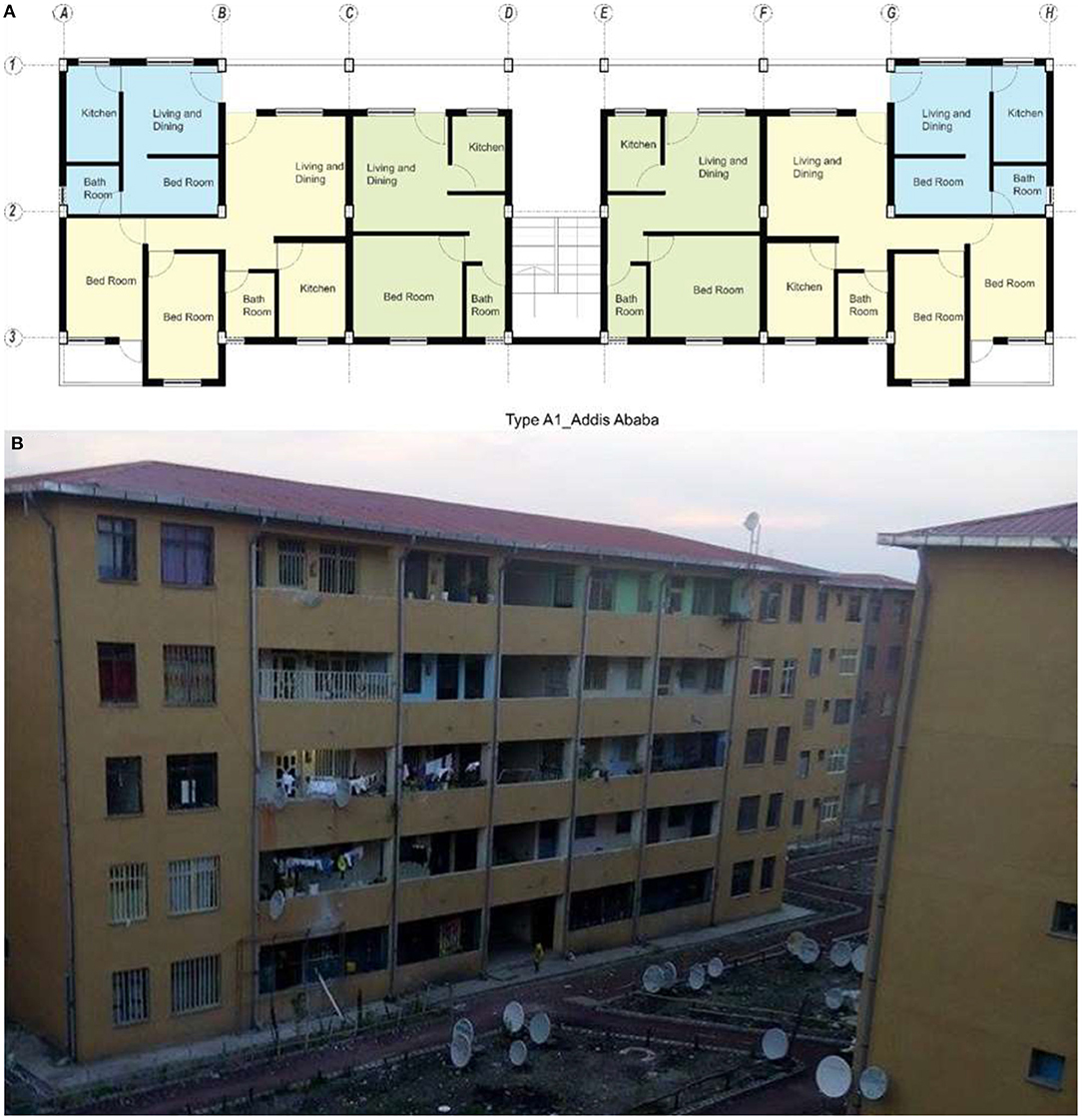
Figure 2. A typical floor layout of a condominium block in Addis Ababa. This building contains studio type apartments (light blue), one-bed type apartments (light green), and two-bed type apartments (light yellow). (A) Floor plan, (B) Photograph of the building (Photo by Mekides Worku).
Figure 2B presents a photograph of the building discussed above (Figure 2A). This photograph is included here for visualization purposes and does not represent all houses surveyed.
Statistical Multivariate Clustering
Unsupervised clustering algorithms are broadly divided into hierarchical, and partitional (Jain, 2010). Hierarchical methods create nested clusters either by using agglomerative (AHC) or divisive (DHC) techniques. The k-means algorithm is one of the widely used partitional clustering techniques. Compared to other methods the k-means method performs well for large datasets (Kidson, 2000). The k-means clustering algorithm divides n points in p dimensions into K clusters through minimizing the within-cluster sum of squares (Hartigan and Wong, 1979). It works by combining two steps: first the initial cluster centroids are estimated, and then the distance between cluster centroids and data points are calculated (Malinen et al., 2014). Cluster centroids are moved each time a new iteration is run until the centers become stationary. The first seed location is taken randomly while the rest are taken by using an optimized initialization technique also known as k-means++ (David and Vassilvitskii, 2006) which ensures separation between seeds in the attribute space. Multiple iterations are tested before final decision is made. The algorithm uses Euclidean distance to group data points (Arora et al., 2016). Euclidean distance estimates the distance between object (i) and group centroid (C) as:
Multivariate clustering results in varying clusters even while using the same data due to the randomness of initialization. A measure of effectiveness is required to ensure the accuracy of the clustering.
Cluster Evaluation
There is no unified technique to ascertain the accuracy of unsupervised classifications. The difficulty arises from the variations in the clustering algorithms, methods, and input variables (Kumar et al., 2006). Another reason is that in unsupervised techniques there is no prior knowledge about the type and number of classes. In this work, accuracy of clustering is evaluated using two methods: pseudo-f-statistic is used to solve the number of groups problem, and building performance assessment is used to evaluate the clustering robustness.
Pseudo-F-Statistic
CH pseudo-F-statistic is an indicator to measure the grouping effectiveness and suggest optimum number of clusters (Caliński and Harabasz, 1974). It is a ratio reflecting within-group similarity and between-group difference. Higher pseudo-f-statistic values indicate ideal number of classes. The ratio is expressed as:
Where:
SST measures the total sum of squared differences, and SSE represents sum of the squared errors in ith group, reflects within-group similarity.
where, n is the number of features. The number of features in group i is given as ni, while nc stands for the number of classes (groups), and nv is the number of variables used to group features. represents the value of the kth variable of the jth feature in the ith group, and is the mean value of the kth variable in group i. SST is also calculated using a similar equation but substitutes the mean value of the kth variable, () instead of .
Building Energy Performance Assessment
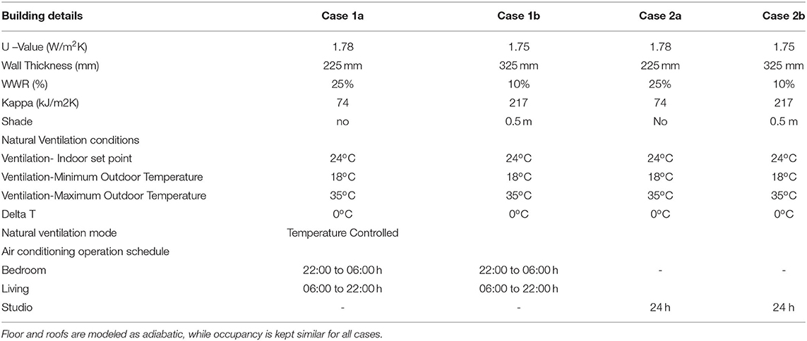
In recent years, building energy performance is being used as an indicator to evaluate the relevance of climate zones. One such attempt uses the mean percentage of misclassified areas (MPMA) to identify overlap of climate zones based on discomfort hours (Walsh et al., 2018). This method demonstrated good results when the number of classes is few (2-4 zones) and the geographic area is small. In a similar note, Xiong et al. (2019) used building heating and cooling load to verify a hierarchical climate zoning. In this study, validation of climate zoning is done through a statistical comparison of heating and cooling DDH, and EPI. Two residential units from the Integrated Housing Development Program of Ethiopia are modeled using energyplus software tool. The first (case 1) is a one-bed room condominium house. The second (case 2), is a single room studio. Two alternatives a low mass (case 1a and 2a) and a high mass (case 1b and 2b) are generated. The low mass buildings are modeled according to the existing specifications of the integrated housing development program of Ethiopia (Table 1). High mass building is generated by modifying kappa value (κ) of walls without altering the U-value and reducing the window-to-wall ratio (WWR) as shown in Table 1. Hourly simulations are performed at 1,490 locations across Ethiopia with an approximate grid interval of 27 x 27 km. The hourly weather data for simulations are synthesized using Meteonorm software tool verified with available ground station data. For each location, simulations are performed for four cases (cases 1a, 1b, 2a, and 2b) operated in free running (natural ventilation) and mixed mode scenarios. This resulted in 11,920 simulation runs. DDH and EPI are extracted from the simulation output using a python post processing script developed by the authors. The results are interpolated using the geospatial analyst tool in ArcMap 10.5.
The discomfort degree hours are estimated as the difference between the adaptive comfort neutral temperature and the zone air temperature. Neutral temperature is calculated from the running mean outdoor temperature through Nicol and Humphrey's equation (Nicol and Humphreys, 2010). Upper and lower comfort temperature limits are determined by adding ±3°C for moderate expectation, as demonstrated by Rajasekar et al. (2015). The whole process was automated using a python post-processing script to reduce errors. The cooling DDH is the cumulative fraction of the inside air temperature that is more than adaptive comfort neutral temperature. Heating DDH is the cumulative fraction of indoor temperature that is less than the adaptive comfort neutral temperature. EPI is the annual energy consumption of a building per unit area in kWh/m2/year (BEE, 2017).
Bioclimatic Zoning
Bioclimatic zoning is performed using Mahoney's method. This method takes monthly temperature, humidity, and precipitation data to analyze thermal severity, identify remedial actions (indicators), and recommend passive building design strategies. This method is suitable for applications on high-resolution monthly data.
Uncertainties in Multivariate Clustering
Uncertainties in cluster analysis can occur due to a combination of factors. Among these are uncertainties due to methodological, latent, and information biases (Fovell and Fovell, 1993). The methodological biases are discussed in section Data Selection and Processing above. Measurement related errors are also dealt with through standardization of the variables in the data pre-processing stage.
Data Related Errors
Two types of climate data are used in the study. The first type of data is a monthly spatial raster and vector data. Root mean square error (RMSE) of Tmax is 1.29°C, while Tmin has an RMSE of 1.39°C, and Iμ 1.45 MJ/m2. Errors associated with RH is reported as the square root of generalized cross validation (RTGCV). Over the domain of North Africa including Ethiopia, monthly RTGCV of RH is reported between 4.6 and 5.6% (New et al., 2002). Further interpolation of RH from 10' to 30” spatial resolution results in RMSE below 0.6%. The second type of data is TMY datasets synthesized from Meteonorm for hourly simulation of building performance. Meteonorm uses a combination of interpolation and stochastic models (Meteonorm, 2018). Errors of interpolation associated with the yearly means of these datasets, as given in the Meteonorm handbook II are discussed here. Cross-correlation of measured and interpolated values is used to calculate the RMSE for individual variables. Accordingly, relative RMSE of Iμ over Africa is reported as 7.4% while RMSE of temperature is estimated at 1.8°C.
Results
Climate Severity
In Ethiopia, TAμ varies from 12 to 30oC. RHAμ varies from 45% to 76%. IAμ varies between 4.8 KWh/m2/day and 6.4 KWh/m2/day. The central parts of the country are characterized by highlands and plateaus resulting in lower temperatures. An exception to this is the central rift valley that intersects the country in a northeast to southwest axis. Regions in the rift valley exhibit warm to hot temperatures with varying humidity. The highest values of IAμ occur in the eastern and northern parts of the country.
The variations of temperature range (ΔT) indicate both spatial and temporal differences (map not included). Some parts of Tigray and Amhara regional states exhibit high levels of ΔT (>15°C) in winter as well as summer. Some climate severity indicators like the Mahoney's method consider a ΔT that is >10°C as high. Accordingly, only small parts of the country in the Northeast indicate low levels of temperature swings in January and western and southwestern regions in June.
Thermal Performance Measurement of Representative Residential Buildings
The types of houses studied in Addis Ababa, and Bahir Dar share common characteristics. For one, these houses are public condominiums constructed under the IHDP scheme. These buildings have similarities in design, construction materials, and overall layout of the buildings themselves. The site settings of these buildings also share a similarity. Both sites are located in outrebounds of the respective city and have an open plan with ample spacing between buildings allowing for unobstructed access to sunlight and air movement. Keeping these factors in mind, a direct comparison of thermal characteristics between Tdiff, ΔT, and Td of all houses in these locations is made.
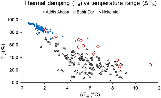
A general comparison shows the variation in thermal performance across cities and similarity within a given city. A thermal damping comparison between the three locations indicate that there is a visible difference between Td in all three locations. In Addis Ababa, the mean Td is 85%, while Td in Bahir Dar is near 60%. Nekemte houses have the lowest Td at <40%.
Figure 3 presents ΔTin against Td of all locations. Houses in Addis Ababa have a short range of ΔTin as well as Td. On the other hand, Bahir Dar houses show the broadest range of ΔTin, while Nekemte houses have a larger spread indicating a weak relationship between ΔTin and Td.
Since the houses in Addis Ababa demonstrated a better thermal performance, a representative house is selected for further analysis through simulations.
Climate Zoning Through Multivariate Clustering
Principal Components Analysis
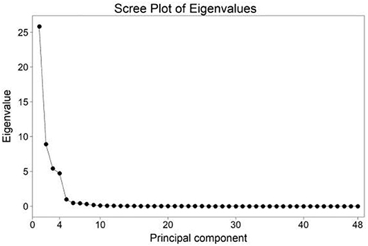
A strong correlation among temperature variables is reflected in the resulting principal components. Optimum number of PCs is estimated using the scree plot. As indicated in Figure 4, the first four PCs are well-separated from the rest. Among 48 layers, four dimensions in the component space account for 93.7% of the variance. Individually, PC1, PC2, PC3, and PC4 account for 53.9, 18.6, 11.3, and 9.9% of the variance respectively. The component loadings reveal the variable groups represented in each extracted PC (Appendix a).
The component loading on the first PC explains Tmax and Tmin of all months. PC two explains RHμ and August Iμ at |R| > 0.60. PC 3 represents Iμ of the months March to June and October to November. The fourth PC shows correlation with late summer RHμ and winter Iμ. Additionally, the communality shows all input variables are well-represented (> 84%) in the extracted PCs. The variable with the lowest variance explained by all PCs is Iμ for November at 72%, followed by RHμ of September at 76%.
The latent variables on the extracted PCs are shown in Appendix b (PC1 to PC4) while the last principal component before extraction (PC48) is displayed for comparison.
Climate Clustering
Grouping is performed iteratively to determine the optimum number of groups inherent in the data. At each stage (number of groups k = 2,…15), 10 iterations are run each yielding a different pseudo-f-statistic value (CH index). The highest mean pseudo-f value is used to determine the optimum number of groups. Based on the pseudo-f-statistic, a 10 class-clustering yields the best results for the current data. However, the differences between 6 and 10 group classification is minimal. In order to investigate this the clustering is repeated by varying the number of groups from 6 to 13. The 6-group classification results in a much-generalized climate zoning and fails to highlight sub zones. On the other hand, any classification that has more than 10-groups is left out due to smaller mean pseudo-f-statistic.
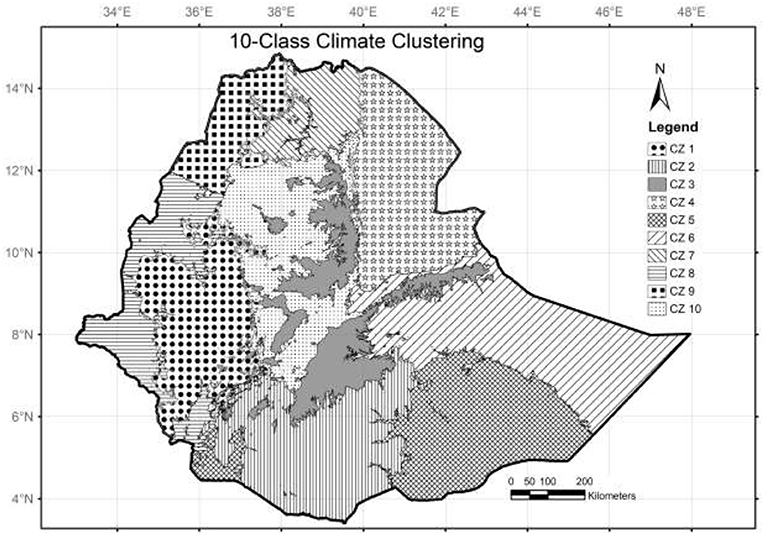
Figure 5 presents the final climate clustering of Ethiopia obtained by this method. The country is grouped into 10 zones based on the highest mean CH index. Some of the zones such as CZ3 and CZ4 correspond to the altitude. However, some of the larger geographical swathes with similar altitude are sub categorized. For instance, climate zones CZ8 and CZ9 in the western lowlands have a similar elevation. This is in contrast with the existing agro ecological climate zoning, which groups geographies based on altitude similarity.
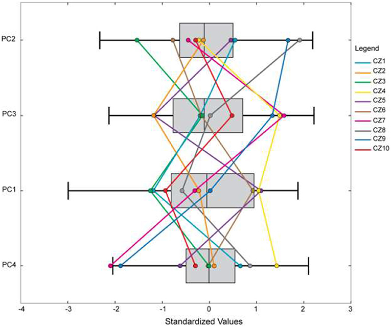
A parallel box plot of principal components used for the clustering is presented in Figure 6. The graph indicates the overlap and separation between each class in terms of the four PCs. It is evident that each group is separated from others at least in one input (PC). The use of optimized seed initialization proves significant by producing less variability of pseudo-f-statistic values as compared to random seed selection. The difference between the maximum and minimum CH index values is 68,187 for random seed selection, and 40,656 for optimized seed selection.
Cluster Evaluation Through Pseudo-F-Statistic
A statistical summary of pseudo-f-statistic values for groups between 2 and 15 is presented in Appendix c. The f-statistic values remain significantly lower for K < =4. On the other hand, for K > 10 these values show a decreasing trend. Since the maximum and minimum values represent extreme conditions, the highest mean value is considered to be better in the current analysis.
Climate Profile of the New Zones
A statistical summary of TmaxAμ, TminAμ, RHAμ and IAμ of the proposed climate zones is presented in Figures 7A–D. As indicated, a difference between medians and distributions are observed.
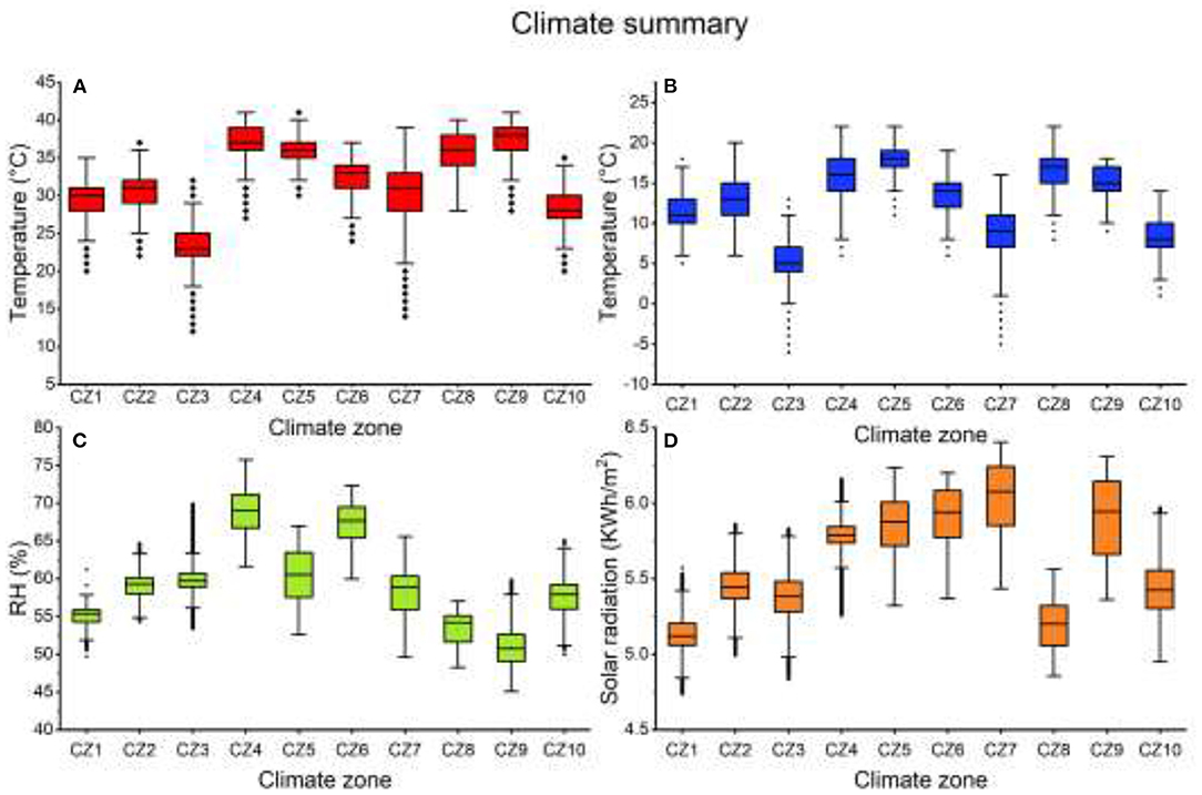
Figure 7. Annual climate summary of new climate zones: (A) maximum temperature; (B) minimum temperature; (C) mean relative humidity; (D) mean solar radiation.
Assessment of Clusters Through Building Simulations
The robustness of the climate zones is verified by comparing the spatial profiles of DDH and EPI. The purpose of this is to test if there is a significant difference in cooling DDH, heating DDH, and EPI between each of the proposed climate zones. It works under the assumption that different climate conditions lead to varying levels of discomfort and thermal performance requirements for a similar building.
Validation of the Base Case
The correlation between the measured outdoor temperature and relative humidity and the locations outdoor climate data is tested. The result shows a significant relationship. For instance, in Nekemte, a simple regression analysis of Tout between measured and climate station data shows a positive correlation (R2 = 0.94) and RHout shows a positive correlation (R2 = 0.92). A paired sample t-test shows, at the 95% CI, the differences between measured Tout and station data Tout are <0.2°C.
Validation of the model is performed on the low-thermal mass 1-bed type apartment (Case 1a). The inside air temperature taken from the field measurement in Addis Ababa (Haile Garment condominium site) is compared with the same room's simulated Tin. Climate data for the simulation is selected from a nearby location to the actual location of the building. Since the simulation model is designed according to the existing building, the validation doesn't include different scenarios (for instance, optimizing various aspects of the model to enhance performance).
Figure 8A presents a line graph comparing the base case's maximum inside air temperature (Case 1a). The result shows that the model fits the measured values significantly. At 95%CI, the difference between measured and simulated Tin_Max is between 0.4 and 1.2°C. A 2-sample standard deviation test for the measured Tin_Max and simulated Tin_Max is performed. The result shows at the 0.05 level; there is no significant difference between standard deviations of measured Tin_Max and simulated Tin_Max (P = 0.431). A simple regression analysis between Tin_max measured and Tin_max simulated indicated a positive correlation (r = 0.69).
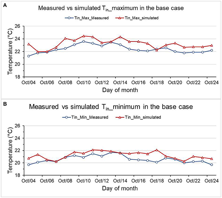
Figure 8. Comparison between measured vs. simulated (A) Tin maximum of Case 1a, and (B) Tin minimum of Case 1a.
A similar analysis on measured and simulated Tin_Min is performed. At the 95%CI, the difference between Tin_Min measured and Tin_Min simulated is below 1.01°C at the highest. Once again, a 2-sample standard deviation test for the measured Tin_Min and simulated Tin_Min is performed. The result shows at the 0.05 level; there is no significant difference (P = 0.43). Figure 8B compares simulated and measured minimum inside air temperatures in Case 1a.
The differences observed above do not solely result from the error in modeling. The raw climate data itself has some inherent differences from the actual measured outdoor climate. The difference stems from (a) climate data for simulation represents a typical meteorological year (TMY) while measured data only represents instant data. (b) the meteorological stations are not located at the building site, and slight variations are expected. Considering these, the building model is validated for further batch processing and analysis.
Limitations
Though the houses used in this analysis are considered representative of emerging residential trends in the country, they are not enough to account for the vast traditional building practices throughout Ethiopia.
Cooling Degree Discomfort Hours
The cooling DDH in this context indicates hot thermal stress that requires cooling. Figure 9 presents the geo-spatial profile of cooling DDH for case 1a, 1b, 2a, and 2b.
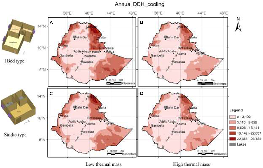
Figure 9. Maps of annual total cooling degree discomfort hours (A) case 1a, (B) case1b, (C) case 2a, and (D) case 2b.
A case-by-case analysis of cooling degree discomfort hours partially reveals the variation between some groups. For instance, in (case1a) distribution of cooling DDH for climate zone 3 and 4 show a considerable difference in terms of both medians as well as distribution. However, these variations are not pronounced between other zones, as is indicated between zone 2 and 7.
Heating Degree Discomfort Hours
The heating DDH in this context indicates cold thermal stress which requires heating. Heating DDH is found to significantly vary among the proposed climate zones (figure not included). Testing of similarities and differences in building performance necessitated the building layout and specifications to be kept consistent across all the 1,490 locations. Though it poses certain practical limitations, this is essential for assessing the climate impact. Further discussions and interpretations related to the performance of high mass and low mass buildings at different locations are limited in this paper considering the intent of the simulations.
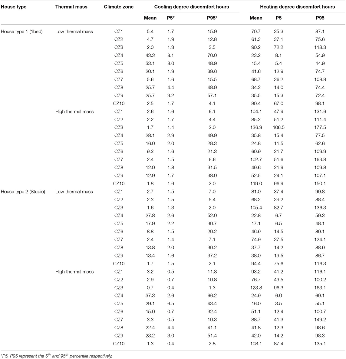
A statistical comparison of climate clusters based on cooling DDH and heating DDH confirms a significant difference among different climate clusters (Table 2).
Energy Performance Index of Climate Zones
The geospatial profile of EPI for the four cases is presented in Appendix d. CZ4 is associated with higher EPI followed by parts of CZ5, CZ6, CZ8, and CZ9. CZ3 is associated with lowest EPI. As indicated in these maps, EPI varies from case to case. To understand the relationship between the climate zones and combined EPI, mean EPI of all cases is calculated (maps not included). The results show similar trends for individual cases.
Figure 10 presents the case wise statistical summary of annual EPI for the proposed climate zones. These results highlight the statistical difference in EPI between climate zones and reinforce the findings presented in Figure 10. CZ4 and CZ5 have higher EPI values across all cases. However, CZ4 shows wider distribution from the mean compared to CZ5. Compared to all zones CZ6 has the widest distribution of EPI. A further investigation of cooling DDH and heating DDH of this particular climate zone indicates high seasonal variability. Climate clusters CZ4 and CZ5 show higher mean EPI while CZ2 and CZ10 show lower mean EPI values.
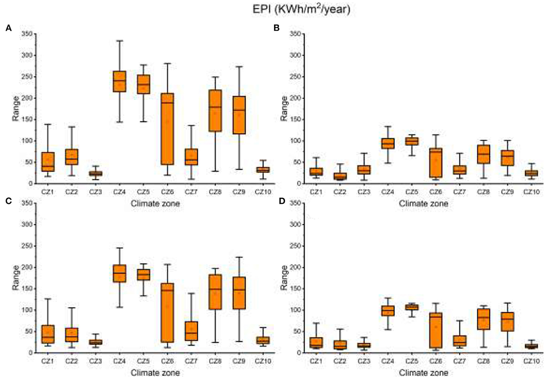
Figure 10. Energy performance index (EPI) comparison (A) case 1a, (B) case1b, (C) case 2a, and (D) case 2b.
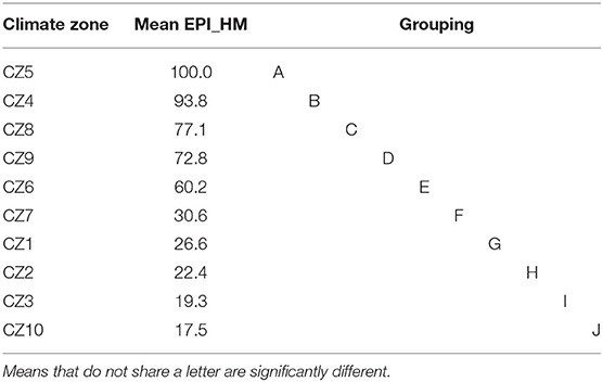
A one way between-clusters ANOVA of EPI shows significant differences among the means at the p = 0.05 level. Additionally, pairwise comparisons aimed to analyse the overlap or separation of clusters based on EPI show significant differences (P < 0.001) between each cluster. Table 3 presents the climate zone wise EPI summary for case 2 as an example. At the mean and 95% confidence interval EPI of every cluster is significantly different. Similar results are observed for the other cases (case 1, 3 and 4).
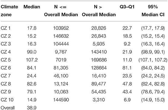
Mood's median test is performed to check the separation between clusters. In this test, median values of EPI for case 4 are compared across climate clusters. At p = 0.05 level the medians of EPI are significantly different across climate zones with (P < 0.001). Statistical summary of medians is presented in Table 4. The Mood's median test does not assume normality.
Bioclimatic Zoning Through Mahoney's Method
The bioclimatic zoning of the country represents the overall passive design strategies recommended individually. Each zone represents places that share similar sets of passive design strategies and in turn, similar climatic preconditions. The eight recommended specifications (a-h) are overlaid with solar radiation groups to create the final bioclimatic strategy group (Figure 11). The methods and resulting bioclimatic zones are documented in a previous work (Zeleke and Rajasekar, 2020). Here the bioclimatic zoning is presented to provide a comparison.
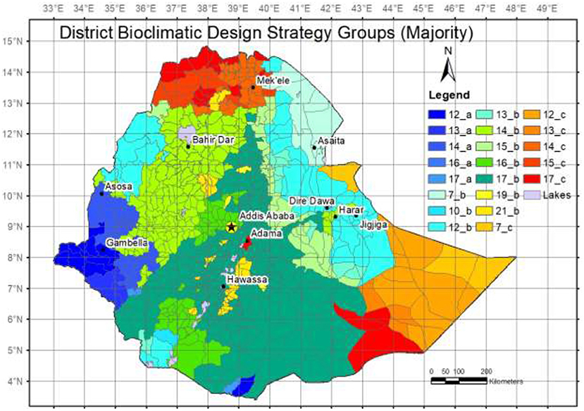
Figure 11. District-level discretization of modified bioclimatic strategy groups (An expanded legend is presented in Appendix e).
Comparative Analysis Between the New Climate Zones and Bioclimatic Zones
This section presents a comparison between bioclimatic zones and the new climate zones in Ethiopia. Each climate zone includes a minimum of five bioclimates zones. Since the number of bioclimate zones is higher than climate zones, this result is not unexpected. This comparison is performed after discretizing both datasets to the district level administrative boundary. Six bioclimatic zones (16a, 7b, 10b, 19b, 13c, and 14c) are found in single climate zones. However, some bioclimatic zones such as 17b are found in as many as seven climate zones.
Energy Efficient Design Strategy Recommendations for Climate Zones
Based on the results of this research, the following general strategies are recommended. In colder climate zones, including CZ3 and CZ10, the use of passive solar heating is encouraged. This is especially important in CZ7, where the cold climate is complimented with relatively high solar radiation. In hotter zones such as CZ4, design strategies that maximize natural ventilation and solar shading are recommended. In extremely cold zones (CZ3) where passive solar heating is unattainable and extremely hot humid zones, HVAC can be used coupled with high thermal mass design. A list of useful bioclimatic strategies for each climate zone is summarized based on the statistical majority (Appendix f). This analysis is meant to provide a simplified representation of design strategy combinations in each climate zone. However, since most of the climate zones cover large geographic areas, a more comprehensive summarization of strategies as well as climate zones to the smallest administrative boundary is performed (table not included).
Conclusions
This study presented a multivariate climate clustering of Ethiopia using high-resolution climate datasets for building energy performance applications. The clustering was performed using the k-means algorithm coupled with the k-means++ initial cluster centroid selection method. Reduction of redundant variables was performed using PCA and four PCs were extracted (Figure 4). Calinski-Harabasz pseudo-f-statistic identified the optimum number of groups as 10 (Appendix c). The use of optimized seed initialization proves significant by producing less variability of pseudo-f-statistic values as compared to random seed selection. The optimized algorithm results in robust climate clusters with resemblances to known climate zones with extreme features while introducing new zones. Robustness of the proposed climate clusters is evaluated by analyzing the cooling DDH, heating DDH and EPI of representative residential cases. These values are obtained through 11,920 runs of building energy simulations performed by considering alternate building layouts, thermal characteristics and operational scenarios for 1,490 locations across Ethiopia. A significant difference in DDH and EPI between climate zones was demonstrated. This study highlights the need to include monthly maximum and minimum temperatures, mean relative humidity and mean solar radiation in the climate zoning for building energy efficiency purposes. The use of multivariate clustering on a high-resolution climate data can be a better alternative to station based clustering used in combination with other supervised interpolation techniques, which might increase uncertainties. The results of this research can be used as a step toward building performance regulations related to building performance, energy efficiency, and usage and will have a potential effect on architectural and urban design for Ethiopia. The results of this study can be used to inform design at the front end and drive the adaptation of climate responsive strategies. However, further tests incorporating other building types and operational characteristics are essential for evolving thermal performance criteria for the proposed climate zones.
Limitations of the Study
This study is limited to exploring a data-driven climate classification of Ethiopia for building energy performance applications. The dimension reduction technique adopted in the study (PCA) assumes a linear relationship between climate variables. The study did not take into account the effects of vegetation cover, availability of open spaces, and differences of rural/urban microclimate due to urban heat island. The effects of the number of residents on heating/cooling is also not investigated.
Data Availability Statement
The raw data supporting the conclusions of this article will be made available by the authors, without undue reservation.
Author Contributions
All authors contributed in the concept, design, analysis, and writing of the manuscript.
Conflict of Interest
The authors declare that the research was conducted in the absence of any commercial or financial relationships that could be construed as a potential conflict of interest.
Publisher's Note
All claims expressed in this article are solely those of the authors and do not necessarily represent those of their affiliated organizations, or those of the publisher, the editors and the reviewers. Any product that may be evaluated in this article, or claim that may be made by its manufacturer, is not guaranteed or endorsed by the publisher.
Acknowledgments
The authors are thankful to the Indian Institute of Technology Roorkee, India, for providing necessary facilities. The authors would like to thank the Ministry of Education of Ethiopia for providing a study abroad fellowship for one of the authors.
Abbreviations
Tmax, mean monthly maximum temperature [°C]; Tmin, mean monthly minimum temperature [°C]; Tμ, mean monthly minimum temperature [°C]; ΔTout, monthly mean temperature range [°C]; TmaxAμ, annual maximum temperature [°C]; TminAμ, annual minimum temperature [°C]; TAμ, annual mean temperature [°C]; ΔTAμ, annual mean temperature range [°C]; RHAμ, annual mean relative humidity [%]; RHμ, monthly mean relative humidity [%]; IAμ, annual mean solar radiation [kWh/m2]; Iμ, monthly mean solar radiation [kWh/m2]; Tn, neutral temperature [°C]; WWR, window-to-wall ratio [%]; U-Value, thermal transmittance [W/m2K]; Kappa, thermal mass [kJ/m2K]; DDH_heating, heating degree discomfort hours; DDH_cooling, cooling degree discomfort hours; EPI, energy performance index [kWh/m2/y]; RMSE, root mean square error; CH index, Calinski-Harabasz pseudo-F-statistic; PC, principal component; PCA, principal components analysis; SST, total sum of squared differences; SSE, sum of the squared errors; CZ, climate zone.
References
Anyadike, N. C. (1987). A multivariate classification and regionalization of West African climates. J. Climatol. 7, 157–164. doi: 10.1002/joc.3370070206
Arora, P., and Deepali Varshney, S. (2016). Analysis of K-Means and K-Medoids algorithm for big data. Phys. Procedia 78, 507–512. doi: 10.1016/j.procs.2016.02.095
Ashrae Standard (1999). Energy standard for buildings except low-rise residential buildings. ASHRAE/IESNA Stand. 2010, 404–636.
Attia, S., Lacombe, T., Rakotondramiarana, H. T., Garde, F., and Roshan, G. R. (2019). Analysis tool for bioclimatic design strategies in hot humid climates. Sustain. Cities Soc. 45, 8–24. doi: 10.1016/j.scs.2018.11.025
Badraddin, A. (1997). Climatic classification of Saudi Arabia: an application of factor - cluster analysis. GeoJournal 41, 69–84. doi: 10.1023/A:1006827322880
Bai, L., Cheng, X., Liang, J., Shen, H., and Guo, Y. (2017). Fast density clustering strategies based on the k-means algorithm. Pattern Recognit. 71, 375–386. doi: 10.1016/j.patcog.2017.06.023
Beck, H. E., Zimmermann, N. E., McVicar, T. R., Vergopolan, N., Berg, A., and Wood, E. F. (2018). Present and future köppen-geiger climate classification maps at 1-km resolution. Sci. Data 5, 1–12. doi: 10.1038/sdata.2018.214
BEE (2017). Energy Conservation Building Code, 2017. Bureau of Energy Efficiency, Ministry Of Power, New Delhi, India.
Bodach, S. (2014). “Developing Bioclimatic zones and passive solar design strategies for Nepal,” in 30th International PLEA Conference (Ahmedabad), 1–8.
Brager, G. S., and de Dear, R. J. (1998). Thermal adaptation in the built environment: a literature review. Energy Build. 27, 83–96. doi: 10.1016/S0378-7788(97)00053-4
Caliński, T., and Harabasz, J. (1974). Communications in statistics - theory and methods. Commun. Stat. 3, 1–27. doi: 10.1080/03610927408827101
Carvalho, M. J., Melo-Gonçalves, P., Teixeira, J. C., and Rocha, A. (2016). Regionalization of Europe based on a K-Means cluster analysis of the climate change of temperatures and precipitation. Phys. Chem. Earth 94, 22–28. doi: 10.1016/j.pce.2016.05.001
Chang, C., Zhu, N., Yang, K., and Yang, F. (2018). Data and analytics for heating energy consumption of residential buildings: the case of a severe cold climate region of China. Energy Build. 172, 104–115. doi: 10.1016/j.enbuild.2018.04.037
Chen, D., and Chen, H. W. (2013). Using the Köppen classification to quantify climate variation and change: an example for 1901-2010. Environ. Dev. 6, 69–79. doi: 10.1016/j.envdev.2013.03.007
Daly, C. (2006). Guidelines for assessing the suitability of spatial climate data sets. Int. J. Climatol. 26, 707–721. doi: 10.1002/joc.1322
David, A., and Vassilvitskii, S. (2006). K-means++: The Advantages of Careful Seeding. Available online at: http://ilpubs.stanford.edu:8090/778/ (accessed December 18, 2008).
DeGaetano, A. T. (1996). Delineation of mesoscale climate zones in the northeastern United States using a novel approach to cluster analysis. J. Clim. 9, 1765–1782. doi: 10.1175/1520-0442(1996)009<1765:DOMCZI>2.0.CO;2
Erell, E., Portnov, B., and Etzion, Y. (2003). Mapping the potential for climate-conscious design of buildings. Build. Environ. 38, 271–281. doi: 10.1016/S0360-1323(02)00119-1
Fazzini, M., Bisci, C., and Billi, P. (2015). “The climate of Ethiopia,” in Landscapes and Landforms of Ethiopia, ed P. Billi (Berlin: Springer Nature Switzerland AG), 65–87. doi: 10.1007/978-94-017-8026-1_3
Fick, S. E., and Hijmans, R. J. (2017). WorldClim 2: new 1-km spatial resolution climate surfaces for global land areas. Int. J. Climatol. 37, 4302–4315. doi: 10.1002/joc.5086
Fovell, R. G., and Fovell, M. Y. C. (1993). Climate zones of the conterminous United States defined using cluster analysis. J. Clim. 6, 2103–2135. doi: 10.1175/1520-0442(1993)006<2103:CZOTCU>2.0.CO;2
Gao, X., and Malkawi, A. (2014). A new methodology for building energy performance benchmarking : an approach based on intelligent clustering algorithm. Energy Build. 84, 607–616. doi: 10.1016/j.enbuild.2014.08.030
Geiger, R., and Pohl, W. (1954). Eine neue Wandkarte der Klimagebiete der Erde nach W. Köppens Klassifikation (A new wall map of the climatic regions of the world according to W. Köppen's classification). Erdkunde 8, 58–61. doi: 10.3112/erdkunde.1954.01.04
Hartigan, J. A., and Wong, M. A. (1979). Algorithm AS 136 : A K-means clustering algorithm. J. R. Stat. Soc. 28, 100–108. doi: 10.2307/2346830
Hashemi, F., Smith, G. W., and Habibian, M. T. (1981). Inadequacy of climatological classification systems in agroclimatic analogue evaluations - suggested alternatives. Agric. Meteorol. 24, 157–173. doi: 10.1016/0002-1571(81)90041-8
Iwaro, J., and Mwasha, A. (2010). A review of building energy regulation and policy for energy conservation in developing countries. Energy Policy 38, 7744–7755. doi: 10.1016/j.enpol.2010.08.027
Iyigun, C., Türkeş, M., Batmaz, I., Yozgatligil, C., Purutçuoglu, V., Koç, E. K., et al. (2013). Clustering current climate regions of Turkey by using a multivariate statistical method. Theor. Appl. Climatol. 114, 95–106. doi: 10.1007/s00704-012-0823-7
Jacobeit, J. (2010). Classifications in climate research. Phys. Chem. Earth 35, 411–421. doi: 10.1016/j.pce.2009.11.010
Jain, A. K. (2010). Data clustering: 50 years beyond K-means. Pattern Recognit. Lett. 31, 651–666. doi: 10.1016/j.patrec.2009.09.011
Johnson, R. A., and Wichern, D. W. (2007). Applied Multivariate Statistical Analysis. Hoboken, NJ: Pearson Education, Inc.
Kidson, J. W. (2000). An analysis of New Zealand synoptic types and their use in defining weather regimes. Int. J. Climatol. 20, 299–316. doi: 10.1002/(SICI)1097-0088(20000315)20:3<299::AID-JOC474>3.0.CO;2-B
Kottek, M., Grieser, J., Beck, C., Rudolf, B., and Rubel, F. (2006). World Map of the Köppen-Geiger climate classification updated. Meteorol. Zeitschrift 15, 259–263. doi: 10.1127/0941-2948/2006/0130
Kriticos, D. J., Webber, B. L., Leriche, A., Ota, N., Macadam, I., Bathols, J., et al. (2012). CliMond: global high-resolution historical and future scenario climate surfaces for bioclimatic modelling. Methods Ecol. Evol. 3, 53–64. doi: 10.1111/j.2041-210X.2011.00134.x
Kumar, V., Tan, P.-T., and Steinbach, M. (2006). Cluster Analysis: Basic Concepts and Algorithms. Introduction to data Mining (Pearson India), 488–568.
Lee, W. S., and Kung, C. K. (2011). Using climate classification to evaluate building energy performance. Energy 36, 1797–1801. doi: 10.1016/j.energy.2010.12.034
Malinen, M. I., Mariescu-Istodor, R., and Fränti, P. (2014). K-means*: clustering by gradual data transformation. Pattern Recognit. 47, 3376–3386. doi: 10.1016/j.patcog.2014.03.034
Markus, T. A. (1982). Development of a cold climate severity index. Energy Build. 4, 277–283. doi: 10.1016/0378-7788(82)90057-3
Meteonorm (2018). Meteonorm Handbook, Part II: Theory. Available online at: https://meteonorm.com/assets/downloads/mn80_theory.pdf
Metzger, M. J., Bunce, R. G. H., Jongman, R. H. G., Sayre, R., Trabucco, A., and Zomer, R. (2013). A high-resolution bioclimate map of the world: a unifying framework for global biodiversity research and monitoring. Glob. Ecol. Biogeogr. 22, 630–638. doi: 10.1111/geb.12022
Naveen Kishore, K., and Rekha, J. (2018). A bioclimatic approach to develop spatial zoning maps for comfort, passive heating and cooling strategies within a composite zone of India. Build. Environ. 128, 190–215. doi: 10.1016/j.buildenv.2017.11.029
New, M., Lister, D., Hulme, M., and Makin, I. (2002). A high-resolution data set of surface climate over global land areas. Clim. Res. 21, 1–25. doi: 10.3354/cr021001
Nicol, F., and Humphreys, M. (2010). Derivation of the adaptive equations for thermal comfort in free-running buildings in European standard EN15251. Build. Environ. 45, 11–17. doi: 10.1016/j.buildenv.2008.12.013
Parracho, A. C., Melo-Gonçalves, P., and Rocha, A. (2016). Regionalisation of precipitation for the Iberian Peninsula and climate change. Phys. Chem. Earth 94, 146–154. doi: 10.1016/j.pce.2015.07.004
Pawar, A. S., Mukherjee, M., and Shankar, R. (2015). Thermal comfort design zone delineation for India using GIS. Build. Environ. 87, 193–206. doi: 10.1016/j.buildenv.2015.01.009
Pesaresi, S., Galdenzi, D., Biondi, E., and Casavecchia, S. (2014). Bioclimate of Italy: application of the worldwide bioclimatic classification system. J. Maps 10, 538–553. doi: 10.1080/17445647.2014.891472
Rajasekar, E., Udaykumar, A., Soumya, R., and Venkateswaran, R. (2015). Towards dynamic thermal performance benchmarks for naturally ventilated buildings in a hot-dry climate. Build. Environ. 88, 129–141. doi: 10.1016/j.buildenv.2014.08.011
Ramos, N. M. M., Almeida, R. M. S. F., Simões, M. L., and Pereira, P. F. (2017). Knowledge discovery of indoor environment patterns in mild climate countries based on data mining applied to in-situ measurements. Sustain. Cities Soc. 30, 37–48. doi: 10.1016/j.scs.2017.01.007
Rivas-Martinez, S., Rivas-Saenz, S., and Penas-Merino, A. (2011). Worldwide bioclimatic classification system. Glob. Geobot. 1, 1–638. doi: 10.5616/gg110001
Saxena, A., Prasad, M., Gupta, A., Bharill, N., Patel, O. P., Tiwari, A., et al. (2017). A review of clustering techniques and developments. Neurocomputing 267, 664–681. doi: 10.1016/j.neucom.2017.06.053
Tadesse, M., Alemu, B., Bekele, G., Tebikew, T., Chamberlin, J., and Benson, T. (2006). Atlas of the Ethiopian Rural Economy. Washington, DC: International Food Policy Research Institute (ifpri) Central Statistical Agencyethiopian Development Research Institute.
Thornthwaite, C. W. (1948). An approach toward a rational classification of climate. Geogr. Rev. 38, 55. doi: 10.2307/210739
Unal, Y., Kindap, T., and Karaca, M. (2003). Redefining the climate zones of Turkey using cluster analysis. Int. J. Climatol. 23, 1045–1055. doi: 10.1002/joc.910
Verichev, K., Zamorano, M., and Carpio, M. (2019). Assessing the applicability of various climatic zoning methods for building construction: case study from the extreme southern part of Chile. Build. Environ. 160, 106165. doi: 10.1016/j.buildenv.2019.106165
Walsh, A., Cóstola, D., and Labaki, L. C. (2017a). Comparison of three climatic zoning methodologies for building energy efficiency applications. Energy Build. 146, 111–121. doi: 10.1016/j.enbuild.2017.04.044
Walsh, A., Cóstola, D., and Labaki, L. C. (2017b). Review of methods for climatic zoning for building energy efficiency programs. Build. Environ. 112, 337–350. doi: 10.1016/j.buildenv.2016.11.046
Walsh, A., Cóstola, D., and Labaki, L. C. (2018). Performance-based validation of climatic zoning for building energy efficiency applications. Appl. Energy 212, 416–427. doi: 10.1016/j.apenergy.2017.12.044
Wan, K. K. W., Li, D. H. W., Yang, L., and Lama, J. C. (2010). Climate classifications and building energy use implications in China. Energy Build. 42, 1463–1471. doi: 10.1016/j.enbuild.2010.03.016
Wilks, D. S. (2011). “Principal component (EOF) analysis,” in International Geophysics 519–562. doi: 10.1016/B978-0-12-385022-5.00012-9
Xiong, J., Yao, R., Grimmond, S., Zhang, Q., and Li, B. (2019). A hierarchical climatic zoning method for energy efficient building design applied in the region with diverse climate characteristics. Energy Build. 186, 355–367. doi: 10.1016/j.enbuild.2019.01.005
Zeleke, B., and Rajasekar, E. (2020). “Geospatial thermal stress assessment and a new bioclimatic classification for Ethiopia,” in 11th Windsor Conference: Resilient Comfort (London) 647–660.
Keywords: climate clustering, k-means algorithm, PCA, degree discomfort hours, energy performance index, Ethiopia, bioclimatic zoning
Citation: Zeleke B, Kumar M and Rajasekar E (2022) A Novel Building Performance Based Climate Zoning for Ethiopia. Front. Sustain. Cities 4:684148. doi: 10.3389/frsc.2022.684148
Received: 22 March 2021; Accepted: 05 January 2022;
Published: 08 February 2022.
Edited by:
Anir Upadhyay, University of New South Wales, AustraliaReviewed by:
Sayanti Mukherjee, University at Buffalo, United StatesSisay E. Debele, University of Surrey, United Kingdom
Copyright © 2022 Zeleke, Kumar and Rajasekar. This is an open-access article distributed under the terms of the Creative Commons Attribution License (CC BY). The use, distribution or reproduction in other forums is permitted, provided the original author(s) and the copyright owner(s) are credited and that the original publication in this journal is cited, in accordance with accepted academic practice. No use, distribution or reproduction is permitted which does not comply with these terms.
*Correspondence: E. Rajasekar, cmFqQGFyLmlpdHIuYWMuaW4=
 Belay Zeleke
 Manoj Kumar
 E. Rajasekar