Solar Energy Modeling and Mapping for the Sustainable Campus at Monash University

An increase in energy demands and positive public acceptance of clean energy resources have contributed to a growing need for using solar energy in cities. Solar photovoltaic (PV) deployment relies on suitable locations with high solar energy potential. In the urban context, building rooftops are often considered one of the most available locations for solar PV installation. This work demonstrates a new geospatial-method for spatiotemporal modeling and mapping solar energy potential based on a high-resolution (0.2 m) digital surface model (DSM) and solar radiation dataset. The proposed method identifies building rooftops with a high solar energy potential by using the Solar Analyst (SA) model. The results show that 93.5% of the rooftop area has high solar energy potential in the study area. The annual averaged sum of solar irradiation values is estimated to be 1.36 MWh/m². In addition, the study showed that sloped rooftops facing to the north received up to 30% more incoming solar radiation than other rooftops with different geometry and orientation. The results are validated using recorded energy output data from four existing solar PV systems in the study area. The return on the initial investment of PV systems installation is estimated to be from four to five years.

Introduction

Cities around the world continue to expand and increase in energy demands. These energy demands are usually satisfied by gas, coal, and oil. Nevertheless, conventional fossil fuels are limited sources of energy with a negative impact on the global climate (Bruckner et al., 2014). The most accepted and available renewable energy source in the urban environment context is solar energy. It is considered one of the most environmentally friendly energy sources (Bruckner et al., 2014). Solar photovoltaic (PV) systems are typically deployed on building rooftops. These systems convert solar energy into electric power. In the last few years, solar PV systems have improved technological efficiency with lower costs in manufacturing and installation (Arvizu et al., 2011; Dinçer, 2011; Bruckner et al., 2014). In addition to that, recent studies have shown that solar energy has been positively accepted by local governments, communities and residents (Mey et al., 2016; Sütterlin and Siegrist, 2017). These technological, economic, and social changes will allow solar PV systems to play a crucial role in the sustainable energy future of cities.

Governmental and business organizations are some of the key stakeholders responsible for the implementation of sustainable development policies. These policies require an effective and accurate method for maximizing electric power generation from clean energy resources. Solar energy planning and decision-making rely on accurate and effective geospatial-based methods for determining the most appropriate locations for solar PV systems. One of the main aspects of applying geospatial-based methods in solar energy planning is the ability to accurately analyze spatial data to provide the most suitable location for the employment of PV systems. In addition to that, geospatial methods by using climate and other data can accurately describe different environmental modeling processes related to solar radiation, hydrology, soil, and other natural phenomenon (Goodchild, 1996).

Geospatial-based solar radiation models have been applied in modeling and mapping solar energy potential in the urban landscape. The development and application of these models have been effectively demonstrated by many studies in the past (Dubayah and Rich, 1995; Kumar et al., 1997; Šúri and Hofierka, 2004; Hofierka and Zlocha, 2012; Catita et al., 2014; Freitas et al., 2015; Liang et al., 2015). Studies showed that three main groups of parameters limit modeling and mapping solar radiation potential by applying geospatial methods. These three main groups of parameters are the following: (i) physical, (ii) geographic, and (iii) technical (Izquierdo et al., 2008). Most geospatial-based solar radiation models account for physical and geographical parameters. Physical parameters are associated with atmospheric effects and interaction of incoming solar radiation with Earth's atmosphere. The atmosphere limits the amount of incoming solar radiation from the sun (Chen, 2011; Duffie and Beckman, 2013). The amount of incoming solar radiation mainly depends on clear sky conditions for a given day or period. Geographic parameters such as geographical location, urban density, building height, vegetation, orientation, and shadow effect describe spatial constraints and urban complexity (Izquierdo et al., 2008; Bergamasco and Asinari, 2011; Hong et al., 2016). The complexity of urban landscape usually requires a high-resolution Digital Surface Model (DSM). The DSM is one of the most crucial features for analyzing the solar energy potential in urban environments (Carneiro et al., 2009).

A high-resolution DSM requires high-quality spatial data to model urban landscapes. The quality of urban surface modeling will provide a more accurate estimate of solar energy potential. Technical parameters include technical information and specifications of PV systems such as array arrangement, energy efficiency, power, and size of solar PV modules and nominal power (Izquierdo et al., 2008). Estimating the electric power potential of PV systems requires information about technical parameters. Together with physical and geographical parameters, they provide a set of constraints in solar energy planning. With the complexity of the urban landscape, the geospatial-based method offers a framework for incorporating these three main groups of parameters together with spatial and other data for estimating solar energy potential (Gadsden et al., 2003; Kanters and Wall, 2016; Shafiullah et al., 2016).

In the last few years, the solar modeling and mapping of urban environments was the subject of different studies, with various scale and complexity levels. A case study in Spain effectively introduced a hierarchical approach using data such as land use, population, and building density for the solar energy assessment of available rooftops (Izquierdo et al., 2008). Similarly, a method based on a digitized vector map was applied for estimating the solar PV potential of building rooftops in Piedmont, Italy (Bergamasco and Asinari, 2011). Another case study investigated a solar rooftop energy potential at Leased Federal Airports in Australia by using the Solar Analyst model and DSM derived from 3D imagery (Teofilo et al., 2021). Different case studies have analyzed and examined a high-resolution LiDAR generated DSM for mapping and quantifying solar radiation distribution for rooftops using the Solar Analyst (SA) module in ArcGIS software (Brito et al., 2012; Kodysh et al., 2013; Santos et al., 2014). Similar work investigated impacts of urban texture on spatiotemporal variations of solar energy potential in downtown Houston based on a high-resolution LiDAR DSM and solar flux radiation model, executed through the ArcGIS extension module (Yu et al., 2009). A solar energy assessment study for buildings in downtown San Francisco demonstrated a geospatial-based method that included solar radiation modeling and mapping of building rooftops using a DSM derived from LiDAR data and r.sun model (Li et al., 2015).

One of the main limitations of previous studies is insufficient or missing validation of geospatial-based solar radiation modeling and mapping. For example, most of the studies mentioned in the previous paragraph do not validate solar radiation modeling results. The validation plays an important part in assessing the correctness of the geospatial-based method. This is essential for solar energy planning and investment in large-size and commercial PV systems across the urban landscape. Another limitation is the lack of detail related to providing information about three main groups of parameters required in geospatial-based modeling and mapping process. For example, most of the studies provide insufficient or inadequate transparency associated with setting values for physical, geographical and technical parameters. This work aims to provide a geospatial-based method without the limitations mentioned above.

Monash University is one of the largest universities in Australia. The university has set goals for delivering carbon-free and energy-sustainable campuses by 2030 (Monash University, 2020). Hence, efficient and financially viable solar energy planning is crucial for delivering sustainable goals in the future. The aim of this study is to demonstrate an accurate and effective geospatial-based method to model and map solar energy potential for the sustainable Clayton campus. Unlike previous studies, the proposed method includes a higher level of details about modeling and includes the validation of results. In addition to that, this work provides an estimate about investment return for installing PV systems on all suitable building rooftops in the campus area.

The remainder of the paper is organized as follows. Section Study Area and Data provides information about the study area and research data. In section Method and Implementation, the proposed method and its implementation are explained with a specific focus on three main steps: (i) surface modeling, (ii) solar radiation modeling and mapping, and (iii) validation. Section Results and Discussion looks at modeling results and provides a deeper discussion about validation and uncertainty of the proposed method. In section Electric Power Generation Potential, the estimated electric power potential, and the payback period are calculated for the installation of commercial PV systems on building rooftops in the study area. Section Study Limitations looks at some of the limitations and applications of the proposed method. Finally, section Conclusions concludes with a review and summary of the key findings and opportunities for future research and uptake of the proposed method.

Study Area and Data

Figure 1 illustrates the study area and spatial data. The area is known as Clayton Campus of Monash University located in the southeast of Melbourne metropolitan area. The campus is one of the largest campuses in Australia with more than 30,000 students every year (Monash University, 2020). This area is within a commercial zone and it has a relatively strong urban presence with a high density of tall buildings. Direct solar radiation data were obtained from the Australian Government Bureau of Meteorology (BOM) (Australian Government Bureau of Meteorology (BOM), 2017) through online access for daily and monthly solar radiation measurements from ground meteorological stations close to the study area. Diffuse solar radiation data were obtained by the NASA Langley Research Center Atmospheric Science Data Center (NASA and Langley Research Center Atmospheric Science Data Center, 2017) from Surface Meteorological and Solar Energy (SSE) web portal supported by the NASA LaRC POWER Project.

FIGURE 1

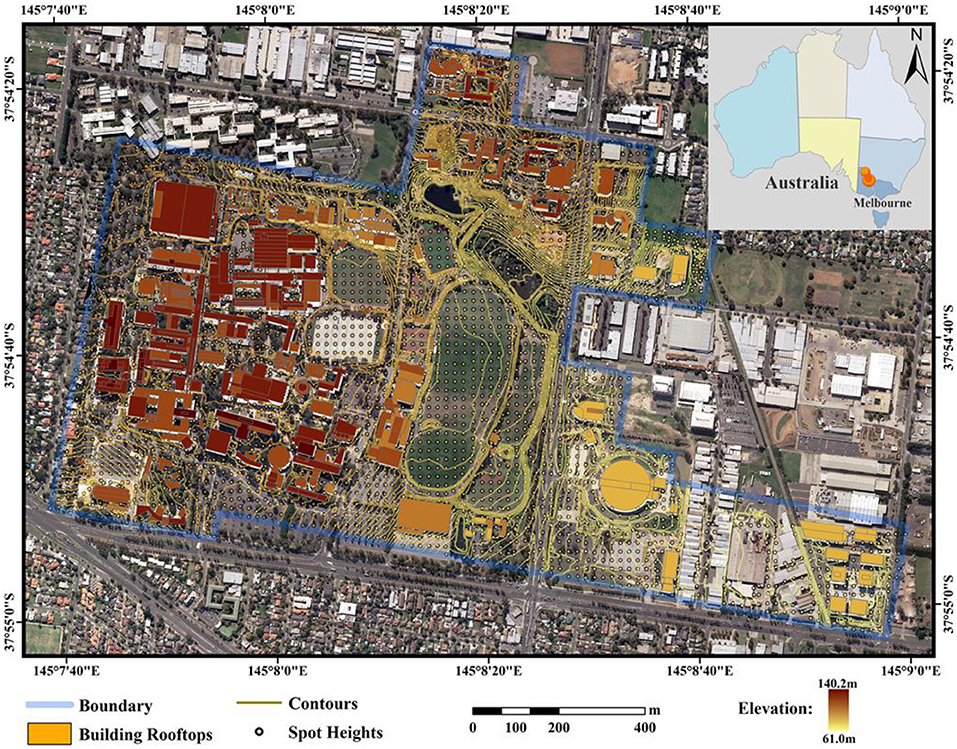
Figure 1. Study area: Monash Clayton Campus, Melbourne, Australia. Spatial data provided by Strategic and Planning Information (SPI) service at Monash University. The data was originally captured and compiled from aerial photography flown on 30 and 31 January 2010. Reference systems used for this study are: (i) horizontal datum: Geocentric Datum of Australia GDA94, (ii) vertical datum: Australian Height Datum (AHD), (iii) map projection in Map Grid of Australia (MGA) Zone 55 and (iv) geoid model Ausgeoid98 for heights (Radosevic et al., 2020).

Method and Implementation

The proposed method illustrated in Figure 2 is divided into three main steps:

1. Surface modeling;

2. Solar modeling and mapping; and

3. Validation of results.

FIGURE 2

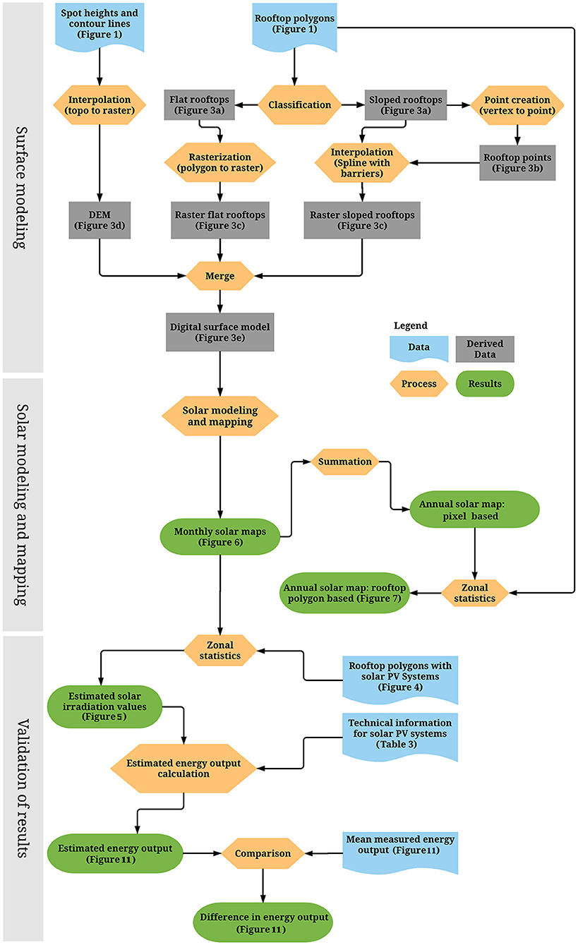
Figure 2. Workflow for the proposed method with three main steps: (i) surface modeling, (ii) solar modeling and mapping, and (iii) validation of results.

In the first step, spatial data is analyzed and processed to model the urban topography of the study area. According to Figure 2 the step includes the following tasks:

• Rooftop polygon classification;

• Rasterization of rooftop polygons;

• Digital elevation modeling; and

• Digital surface modeling.

In the second step, the SA model executes solar radiation modeling and estimates solar irradiation values for building rooftops. The modeling results are illustrated with the following maps:

• Monthly and annual solar radiation maps based on pixel values; and

• Annual solar radiation map based on rooftop polygon values.

In the third step, the model output is validated by conducting the following tasks:

• Estimating energy output from four building rooftops with mounted solar PV systems in the study area; and

• Calculating the difference between the recorded and estimated energy output from four building rooftops with mounted solar PV systems in the study area.

Surface Modeling

In the first step of the proposed method, the main objective is to model and generate a high-resolution DSM of the campus area. This includes the preparation and processing of spatial data depicted in Figure 1. Firstly, a vector spatial dataset representing rooftop polygons in Figure 3A is classified into two different groups: flat and sloped rooftop polygons. This classification is based on height (Z) values of polygon vertices using Autodesk Civil 3D software. Rooftop polygons containing vertices with different Z values are classified as sloped and rooftop polygons including vertices with the same Z values are categorized as flat. Figure 3A shows a considerably larger number of flat rooftops or 81.5% of the total campus' rooftop area. In contrast, the sloped rooftop area covers only 18.5% of the entire rooftop area on the campus.

FIGURE 3

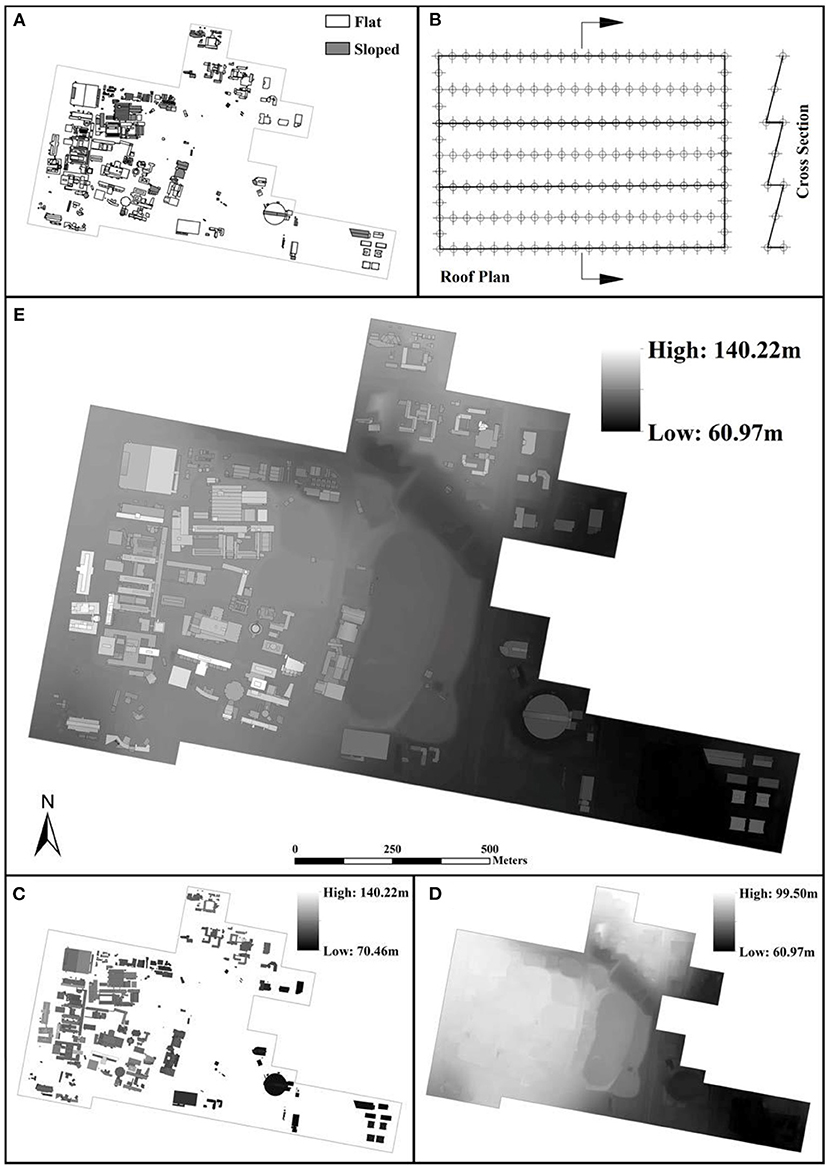
Figure 3. (A) Rooftop polygon classification; (B) sloped rooftop polygon points; (C) raster rooftop polygons; (D) digital elevation model (DEM); (E) digital surface model (DSM) (Radosevic et al., 2020).

After the classification, these two groups of rooftop polygons are converted from vector to raster spatial data format. This process of spatial data manipulations is called rasterizing. In this case study, sloped rooftops are rasterized by creating additional rooftop points from polygon vertices in Autodesk Civil 3D. Each new rooftop point is used for linear interpolation between two points with known Z values. The objective of this task is to create a new set of points to define the geometry of each sloped polygon. Figure 3B shows new rooftop points for converting sloped rooftops from vector to raster spatial data. The conversion is executed by interpolation method Spline with Barriers using polygon boundary as a barrier (Terzopoulos, 1988). Rooftop polygons classified as flat were directly converted into raster data format by ArcGIS software using Polygon to Raster tool (http://pro.arcgis.com/en/pro-app/tool-reference/conversion/polygon-to-raster.htm). Figure 3C depicts all rooftop polygons rasterized into a raster format with 0.2 m spatial resolution.

Secondly, a Digital Elevation Model (DEM) is generated from spot heights and contour data illustrated in Figure 1. The DEM is generated and interpolated by Topo to Raster tool in the ArcGIS Spatial Analyst toolbox (Environmental Systems Research Institute, 2021a). Figure 3D depicts the DEM and configuration of terrain in the study area. Finally, the DSM is created by using the Map Algebra tool in the ArcGIS Spatial Analyst toolbox (Environmental Systems Research Institute, 2021b). The rasterized rooftop polygons and the DEM are merged to create the DSM illustrated in Figure 3E. A color gradient illustrates different height values of the DSM. For example, lighter colors in the gradient demonstrate some of the tallest buildings in the campus area.

Solar Modeling and Mapping

Solar energy assessment across the study area is executed based on the high-resolution (0.2 m) DSM and modeled by the SA module in ArcGIS software. The SA model is based on a spatial solar radiation model developed by Fu and Rich (1999). This model calculates incoming solar radiation based on input such as topographic and radiation parameters. It provides a fast and accurate calculation of direct, diffuse, and global solar radiation. In addition to that, the SA can estimate incoming solar radiation for any specified period (hourly, daily, monthly, or yearly) (Fu and Rich, 2000). The SA model does not account for the reflected component of global solar radiation. Hence, this component is excluded from the calculation of global solar radiation. Nevertheless, the reflected component was considered to be insignificant because of the low value of the average annual surface albedo for the Melbourne region (NASA and Langley Research Center Atmospheric Science Data Center, 2017).

Table 1 defines input parameters for solar radiation modeling with the SA model. Geographic latitude is one of the main geographical parameters required for setting the location of the study area. Time is required for setting the time interval for modeling solar radiation potential. The z-factor is used for correcting calculations in cases when different units of length are used in the z-direction (height) compared to the x, y planar units of the DSM. The type parameter determines the accuracy of the SA model. For diffuse model type, it was selected the standard overcast sky in which the amount of incoming diffuse radiation varies with zenith angles (Fu and Rich, 2000). The transmission of solar energy through the Earth's atmosphere is defined with a transmission proportion index. This physical parameter demonstrates weather conditions for transmission of solar radiation through the sky (Fu and Rich, 2000; Chen, 2011). The monthly averaged transmission index value for all months was set to 0.55 which indicates generally clear sky conditions (Fu and Rich, 2000).

TABLE 1

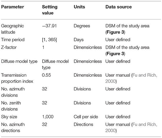
Table 1. Solar Analyst parameters (Radosevic et al., 2020).

The remaining group of parameters in Table 1 defines the spatiotemporal granularity of solar radiation modeling. According to the sun positions during a day, zenith and azimuth divisions define the number of sectors in the sky map (Fu and Rich, 1999, 2000). In this study, the number of divisions was set to 32 to reduce an error in estimating incoming global solar radiation (Li et al., 2016). The sky size is associated with raster resolution of the hemispherical viewshed, sun map and sky map raster maps for calculation of solar irradiation maps (Dubayah and Rich, 1995; Fu and Rich, 1999, 2000).

The number of azimuth directions defines the number of rays to calculate the viewshed. Also, the viewshed calculation includes other topographic parameters such as slope and aspect from the DSM. In addition to that, a shadow effect on solar radiation potential is calculated based on the rooftop elevation value provided by the DSM.

Another important physical parameter in the modeling is a diffuse proportion index. This index determines how much solar radiation is diffused and reflected within Earth's atmosphere (Fu and Rich, 2000; Chen, 2011). A monthly diffuse index is calculated with the following equation:

$\begin{array}{ll}{K}_{\text{d}}=G_{\text{d}}/(G_{\text{b}}+G_{\text{d}})& (1)\end{array}$

The monthly diffuse index demonstrates the ratio of monthly averaged diffuse solar radiation and the monthly averaged clear sky insolation incident on a horizontal surface (Fu and Rich, 1999, 2000). The monthly averaged clear sky insolation incident on a horizontal surface is equal to the sum of the monthly averaged diffuse and beam solar radiation for standard overcast days (NASA and Langley Research Center Atmospheric Science Data Center, 2017). Table 2 presents calculated values for diffuse proportion index, monthly averaged values of diffuse solar radiation, and beam solar radiation for the study area. Parameter setting values shown in Tables 1, 2 were used to configure the model and to estimate the solar radiation potential of building rooftops in the study area.

TABLE 2

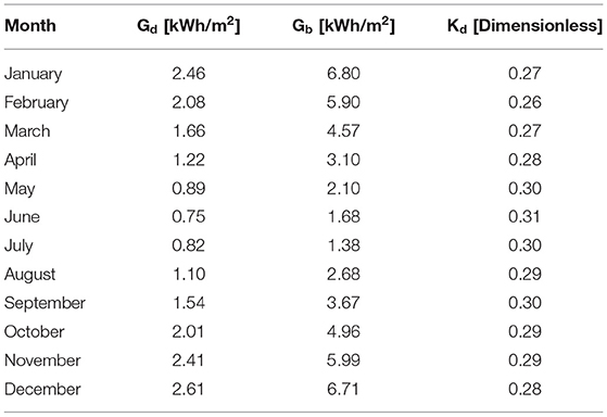
Table 2. Monthly setting values for diffuse proportion index.

Validation of Results

The last main step in the proposed method involved a validation procedure for calculated solar energy potential. The validation was determined by the difference between the mean recorded and estimated energy output per unit area. Estimated values for the energy output were calculated for four building rooftops marked with red color in Figure 4. The values were derived from monthly solar maps in Figure 6.

FIGURE 4

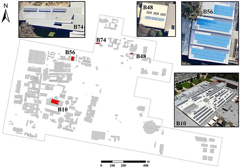
Figure 4. Locations of existing solar PV systems in the study area.

Mean recorded monthly values for energy output were calculated from recorded energy output captured by the existing solar PV systems illustrated in Figure 4. Monthly values for energy output are measured and recorded for solar PV systems mounted at the rooftops of building 10 (B10), building 48 (B48), and building 74 (B74) and obtained online from Sunny Portal website (www.sunnyportal.com). Measured energy output data recorded from the solar PV system mounted at the rooftop of building 56 (B56) was received from Monash University. The data for some months was not available or incomplete. Hence, it was excluded from the validation process.

Table 3 demonstrates a summary of existing solar PV systems in the study area. Solar PV systems mounted at rooftops of B10 and B56 have significantly higher power output capacity and a considerably larger number of solar PV modules (Pn) than solar PV systems mounted at rooftops for B48 and B74. In addition to that, the table shows the rooftop type and commencing dates of solar PV systems, the total area (A_system), tilt, and aspect angles of installed solar PV modules in the study area. Solar PV modules at the rooftop of B56 were mounted directly to the rooftop without additional tilting. Table 2 also provides technical specifications for different solar PV panel types mounted on these four building rooftops in the study area.

TABLE 3

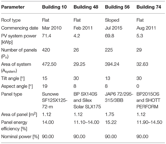
Table 3. Summary information for solar PV systems mounted at four building rooftops.

The estimated monthly averaged global solar radiation on a tilted surface (G_t) was calculated in RETScreen Clean Energy Management software (Natural Resources Canada, 2000). The following parameters were used for the estimation: geographic location (latitude and longitude), aspect, and tilt angle for the existing solar PV systems (Table 3). The estimated monthly averaged global solar radiation on a flat surface (G_h) was obtained by the SA model. Figure 5 summarizes G_t and G_h values from four rooftops with solar PV systems in the study area. Using the estimated G_t and G_h values the tilt factor was calculated according to the following equation:

$\begin{array}{ll}{T}_{\text{factor}}=G_{\text{t}}/G_{\text{h}}& (2)\end{array}$

FIGURE 5

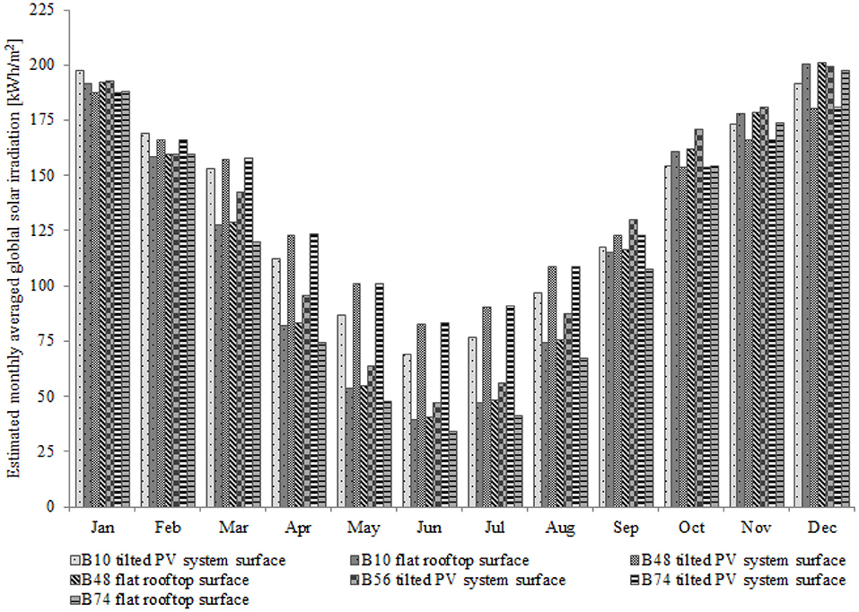
Figure 5. Estimated monthly averaged global solar irradiation on tilted PV system and flat rooftop surfaces of four buildings in the study area.

Monthly estimated solar radiation potential and parameters in Table 3 were used to calculate monthly estimated power output per unit area with the following equation (Singh and Banerjee, 2015):

$\begin{array}{ll}{\text{P}}_{\text{E}}=G_{\text{monthly}}{\text{N}}_{\text{power}}{\text{T}}_{\text{factor}}\text{η}& (3)\end{array}$

Absolute values for the difference (D) between the estimated (P_E) and mean measured (P_M) energy output per unit area were calculated according to the following equation:

$\begin{array}{ll}\left|D\right|=P_{\text{E}}-P_{\text{M}}& (4)\end{array}$

Results and Discussion

Solar Energy Potential of Building Rooftops

Solar irradiation values for each month were estimated in kWh/m² and presented in the 12-month solar map series. Figure 5 demonstrates a monthly variation of solar irradiation values in the Clayton campus. Lower values are presented with yellow color and they dominate through Jun and July. From July solar irradiation value starts to increase and it reaches the highest values illustrated with red color during summer months in December and January.

Twelve monthly solar maps depicted in Figure 6 were aggregated into the annual solar map. Figure 7 depicts the annual solar map. The map also shows the influence of the shadow effect on the annual solar radiation potential. An example of a building is illustrated in Figure 7. Lower rooftop areas of the B11 building with yellow color received significantly less solar irradiation compared to higher rooftop areas marked with red color. The range of annual solar irradiation values shown in the map is from 69.5 kWh/m² to 1548.2 kWh/m² with the mean annual value of 1363.9 kWh/m².

FIGURE 6

Figure 6. Monthly solar maps.

FIGURE 7

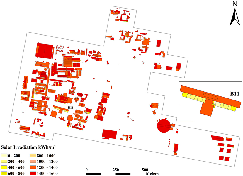
Figure 7. Annual solar map based on rooftop polygons (Radosevic et al., 2020).

The solar energy potential of building rooftops was further analyzed by classification of rooftop polygons based on their solar irradiation values from the modeling. Figure 8A demonstrates a distribution of building rooftop polygons in 8 different categories based on estimated solar irradiation values from the annual solar map. Figure 8B demonstrates that more than 90% of the total rooftop area is included in categories 7 and 8 with high annual solar irradiation values (1,200–1,400 and 1,400–1,600 kWh/m²). Hence, this shows that most of the rooftop area has a high solar energy potential for PV system installation.

FIGURE 8

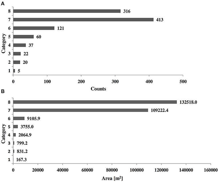
Figure 8. (A) Histograms of building polygon counts with corresponding categories for solar energy potential. (B) Histograms of rooftop polygon area within corresponding categories for solar energy potential.

Solar Energy Potential for Different Rooftop Geometry and Orientation

The electric power generation from rooftop-mounted PV systems may vary due to different rooftop geometry and orientation. This section goes further with rooftop solar radiation modeling by analyzing six different rooftop geometry and orientation. All selected rooftops had no shadow cast from surrounding buildings and vegetation. Figure 9 illustrates six different rooftops in the study area. The rooftops and their properties are the following:

1. Sloped rooftop A with a 15° tilt angle and oriented to the north at an azimuth angle of 24°;

2. Sloped rooftop B with a 12° tilt angle and oriented to the south at an azimuth of 186°;

3. Sloped rooftop C with an 11° tilt angle and oriented to the east at an azimuth angle of 98°;

4. Sloped rooftop D with a 14° tilt angle and oriented to the west at an azimuth angle of 278°;

5. Sloped rooftop E with a 15° tilt angle and oriented to the north at an azimuth angle of 8°; and

6. Flat rooftop F oriented to the north at an azimuth angle of 1°.

FIGURE 9

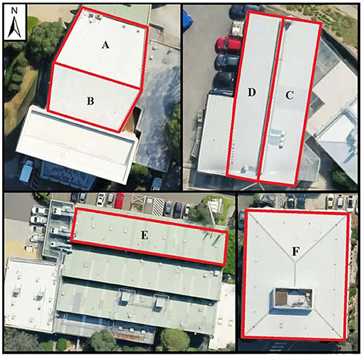
Figure 9. Selected rooftops in the study area.

Estimated results by the Solar Analyst model show that rooftops A and E have the highest annual sum of solar irradiation values between the selected rooftops. Figure 10 graphically represents results from this analysis. The analysis also demonstrates that north-facing rooftop F has a lower annual sum of solar irradiation values when is compared to rooftops A and E. In addition to that, the sloped rooftop B has the lowest solar energy potential between all rooftops. The annual solar irradiation difference between rooftop E and rooftop B is of 345.5 kW/m².

FIGURE 10

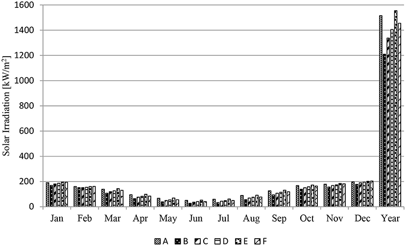
Figure 10. Monthly and annual solar irradiation values for the selected rooftops.

Based on the results from the analysis most suitable rooftops for PV systems deployment are sloped rooftops A and E. In contrast, rooftop B is less likely to be selected for PV system installation from all six rooftops. This assessment also shows that within a year flat rooftops oriented to the north (F) may receive more incoming solar radiation than sloped rooftops oriented to the west and the east (C and D). During winter months sloped rooftops oriented to the north can receive up to 20% more incoming solar radiation than flat rooftops facing to the north. On the annual basis, north-facing rooftops with sloped geometry can receive up to 6% more incoming solar radiation than flat rooftops with the same orientation and up to 29% more than sloped rooftops facing to the south. This analysis demonstrates that the geometry and orientation of rooftops can have a significant impact on potential electric power generation from PV systems.

Uncertainty in Solar Radiation Modeling

Uncertainty may arise at any step of the solar radiation modeling process. Some of the sources of uncertainty may be related to the following: (i) spatial data and the DSM, (ii) parameter setting values, and (iii) inherited uncertainty of the model itself. In this study, high-quality spatial data and DSM were used for the modeling. A high granularity DSM with 0.2 m pixel size was generated demonstrating a minimal uncertainty in terms of spatial data representation. In addition to that, the DSM included sloped rooftops with a minimum level of generalization. In terms of parameter setting values, most of the parameters were set according to the Solar Analyst user manual (Fu and Rich, 2000). The exception is monthly setting values for diffuse proportion index (Table 2) estimated by using solar radiation data provided by NASA Langley Research Center Atmospheric Science Data Center (NASA and Langley Research Center Atmospheric Science Data Center, 2017). For two parameters, sky size and number of azimuth directions, an increase in setting value may provide higher accuracy of estimated solar irradiation values. Nevertheless, the improvement is rather insignificant compared to a longer computational time with higher setting values for these two parameters. Finally, model uncertainty may be another source of errors in the estimated solar radiation potential of the study area. A study conducted by Li et al. (2016) showed that the Solar Analyst has a tendency to slightly overestimate solar irradiation values. In summary, the estimated solar radiation modeling results provide accurate and reliable information for solar energy planning in the study area.

The Difference Between Measured and Estimated Energy Output

In this section, validation results are graphically represented in Figure 11. Figure 11A illustrates the bar chart of monthly estimated (P_E) and mean measured (P_M) energy output per unit area from PV systems mounted on four building rooftops in the study area. The linear graph in Figure 11B demonstrates absolute values for difference (D) in kW/m² between P_M and P_E. Monthly D values are between 0.1 kWh/m² and 2.4 kWh/m² and annual D values are between 1.0 kWh/m² and 3.7 kWh/m². The results show a relatively small difference between estimated and mean measured energy output.

FIGURE 11

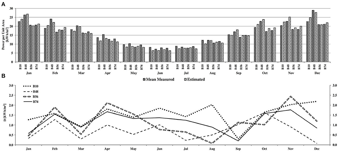
Figure 11. (A) Monthly values for mean measured (P_M) and estimated (P_E) power output per unit area from four building rooftops; (B) the difference in absolute values between P_M and P_E.

The source of errors for validating results can be divided based on two major variables in Equation (4): (i) estimated energy output, and (ii) mean measured energy output. Errors in calculating estimated energy output are directly related to the accuracy of estimated solar irradiation values by the Solar Analyst and tilt factor. Monthly tilt factor values were calculated based on estimated solar radiation data for horizontal and tilted surfaces. The estimated solar radiation data for the horizontal surface was adopted from the modeling. Errors in estimating solar radiation on the tilted surface may be related to errors in modeling and uncertainty in the application of RETScreen Clean Energy Management software (Natural Resources Canada, 2000). Further, errors in calculating mean measured energy output can be directly related to the quality of measured data available on the Sunny Portal website (www.sunnyportal.com). This data depends on monthly recorded energy output from PV systems. For the same period between different years, the monthly recorded energy output may vary because of various weather conditions causing a reduction or increase in solar irradiation exposure.

In summary, the validation showed a relatively low difference between the estimated and mean energy output from four building rooftops. Hence, the estimated solar irradiation values are with a high level of confidence.

Electric Power Generation Potential

The annual potential for electric power generation can be estimated according to the following equation (Gastli and Charabi, 2010):

$\begin{array}{ll}EP=ARRAAF\eta N_{\text{power}}& (5)\end{array}$

Where all parameters and their values are defined and calculated in Table 4.

TABLE 4

Table 4. Definition and values of parameters used in Equations (5) and (6).

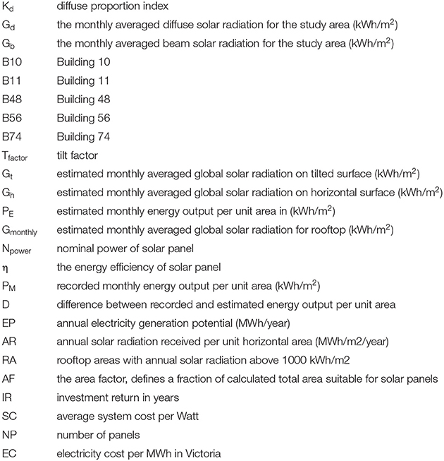
The adopted AR value is the estimated average solar radiation potential from the Solar Analyst model. The RA parameter value is equal to the sum of rooftop areas classified in categories 6, 7, and 8 shown in Figure 7. The AF parameter value is adopted after the inspection of the aerial image of the study area. Rooftops were assessed on their spatial and technical limitations. This includes a tree shadow effect, rooftop complexity, and required space between solar arrays. In addition to that, the energy efficiency and nominal power values of solar panel Trina 250 W were used in the estimation of annual power generation potential. The annual electric power potential from roof-mounted PV systems was estimated to be 23488.24 MWh based on the set of parameters provided in Table 4. From Table 4, it seems apparent that parameter setting values may vary according to different scenarios. Hence, the EP should be only considered as an estimated value.

In the long term, PV systems can offer financial savings and a reduction of electricity costs. The investment return for the installation of commercial rooftop PV systems is estimated by using the set of parameters in Table 4 and the following equation:

$\begin{array}{ll}IR=(SC{P}_{\text{n}})/(UEPEC+R_{\text{FIT}})& (6)\end{array}$

An average commercial PV system installation cost for a rating between 10 and 100 kW is from AU$0.88 to AU$1.10 per Watt in Melbourne (Solar Choice, 2021a). The cost of the PV system installation (SC) is adopted based on a 50 kW commercial PV system per Watt (Solar Choice, 2021a). The energy efficiency and nominal power setting values of the Trina 250 W solar panel were used in the equation above. The total number of panels was estimated by dividing 50% of the available rooftop area by the Trina 250 W solar panel area (1.65 m²). Parameter setting value for used electric power potential during peak time (UEP) was set according to two scenarios. In the first and more optimistic scenario, the UEP is set to be 50% of the yearly peak electricity demand on the Clayton campus. In the second and more pessimistic scenario, the UEP is set to be 25% of the yearly peak electricity demand on the Clayton campus. These parameter setting values were estimated based on electricity consumption data provided by Monash University. Data shows that electricity consumption on the campus during peak time was around 32,000 MWh in 2010 and 2011. The electricity cost in Victoria was set according to a report from the Australian Energy Market Commission in 2020 (Australian Energy Market Commission, 2020). In both scenarios, the amount of annual electric power generation potential exceeded the yearly peak energy demand of the campus. The exceeded electricity was counted as potential revenue from feed-in tariffs (R_FIT). The estimated value for this parameter was defined on the minimum feed-in tariffs rating of 102AU$ per MWh or 10.2 cents per kWh in Victoria for 2021 (Solar Choice, 2021b).

Results from the analysis demonstrate the estimated investment return period for scenario 1 and scenario 2 are 4 and 5 years, respectively. This analysis shows that even by providing only 25% of the yearly peak electricity demands from rooftop PV systems the investment can be financially viable with a relatively short economic return. It is worth mentioning that with the minimum feed-in tariffs rating, a yearly revenue from generating and distributing electricity from PV systems to the national grid may reach almost 1.6 million Australian dollars. This estimate demonstrates only the investment return on the initial cost of PV systems installation at the study area. The other costs associated with the solar PV system are not included in the estimate. These costs may relate to the maintenance and servicing of the system after the installation. In addition to that, this analysis does not account for the deployment of battery storage in the study area.

Limitations of the Study

Primarily, study limitations are associated with limited spatial data related to trees and vegetation in the case study area. With the application of LiDAR (Light Detection and Ranging) data, the accuracy of the solar radiation modeling and mapping may be improved by including a potential shadow cast from tall trees and vegetation. Nevertheless, Figure 1 shows that the presence of tall trees near building rooftops may be insignificant in the study area. Another limitation is that the scope of this study focuses only on the analysis of the solar energy potential of building rooftops. With more detailed spatial data, this analysis can include other urban features such as building facades, concrete pavements, and parking areas present in the study area. One more limitation is associated with energy consumption data. This data included some incomplete information about several buildings in the study area. Also, the available data showed only monthly peak and off-peak energy consumption for every building on the Clayton campus. The average hourly energy demands data for each building would allow for a more accurate estimation of how much solar PV system-generated electricity power may exceed the peak time energy demands.

Conclusions

Deployment of PV systems involves planning and decision-making for their future locations. Hence, a geospatial-based method can play an important part in the planning and installation of future PV systems. The motivation for this case study comes from the growing need to use building rooftops as a place for generating clean and renewable energy. Building rooftops are one of the most suitable urban locations for generating electricity across the urban landscape. In addition to that, buildings powered by renewable energy represent an ultimate goal for the development of sustainable cities in the future.

This paper demonstrates a new geospatial-based method using spatial data for modeling, mapping, and quantifying available solar energy resources for building rooftops in Melbourne urban area. The results show that 93.5% of rooftop area has high solar energy potential. The annual sum of solar irradiation values showed an average estimated value of 1.36 MWh/m² in the study area. In addition to that, the rooftop analysis for different orientations and geometries showed that sloped rooftops facing to the north received up to 30% more incoming solar radiation than sloped rooftops facing to the south. The validation of modeling results showed a relatively small difference between estimated and recorded energy output for four building rooftops in the study area. The monthly difference was in the range between 0.1 and 2.4 kWh/m² and the annual difference between 1.0 and 3.7 kWh/m². The estimated annual electricity generation from 50% of the suitable rooftop area can provide 23488.24 MWh. The investment return of the initial investment in PV systems installation is estimated to be from 4 to 5 years.

The main focus of this research was on demonstrating the new geospatial method for solar energy modeling and mapping for delivering solar energy assessment and planning. Future research may include an analysis of the solar energy potential of vertical surfaces such as building facades. In addition to that, future work may look at PV energy output performance between fixed and PV tracking energy systems.

As a general conclusion, the assessment of solar energy potential provides valuable information to energy planners and decision-makers. The method in this study accurately estimates solar energy resources across specific urban environment contexts. The assessment conducted with this method provides an incentive for solar energy-powered cities in the future.

Data Availability Statement

The data analyzed in this study is subject to the following licenses/restrictions: dataset is owned by Monash University and it is not publicly available. Requests to access these datasets should be directed to peter.jolly@monash.edu.

Author Contributions

NR designed, prepared, conducted analysis and participated in writing introduction, methodology, results, analysis, and conclusions sections. G-JL designed the methodology and analysis and participated in writing introduction, methodology, result and analysis, and conclusion sections. NT designed the methodology and participated in introduction and conclusion sections. XZ designed the methodology and participated in writing results and conclusions sections. QS designed the methodology and participated in writing results and discussion sections. All authors contributed to the article and approved the submitted version.

Funding

This work was supported through the provision of an Australian Government Research Training Program Scholarship. In addition, publication costs for this work were supported by the RMIT Science, Technology, Engineering, and Mathematics College.

Conflict of Interest

The authors declare that the research was conducted in the absence of any commercial or financial relationships that could be construed as a potential conflict of interest.

Publisher's Note

All claims expressed in this article are solely those of the authors and do not necessarily represent those of their affiliated organizations, or those of the publisher, the editors and the reviewers. Any product that may be evaluated in this article, or claim that may be made by its manufacturer, is not guaranteed or endorsed by the publisher.

Acknowledgments

The authors would like to thank Monash University for providing spatial, energy, and solar PV technical data.

References

Arvizu, D., Balaya, P., Cabeza, L., Hollands, T., Jäger-Waldau, A., Kondo, M., et al. (2011). “Direct solar energy,” in IPCC Special Report on Renewable Energy Sources and Climate Change Mitigation, eds O. Edenhofer, R. Pichs-Madruga, Y. Sokona, K. Seyboth, P. Matschoss, S. Kadner, T. Zwickel, P. Eickemeier, G. Hansen, S. Schlömer, C. von Stechow (Cambridge, UK; New York, NY: Cambridge University Press), 333–400. Available online at: https://www.ipcc.ch/site/assets/uploads/2018/03/Chapter-3-Direct-Solar-Energy-1.pdf

Google Scholar

Australian Energy Market Commission (2020). Residential Electricity Price Trends 2020. Available online at: https://www.aemc.gov.au/sites/default/files/2020-12/2020%20Residential%20Electricity%20Price%20Trends%20report%20-%2015122020.pdf

Google Scholar

Australian Government Bureau of Meteorology (BOM) (2017). Climate Data Online. Available online at: http://www.bom.gov.au/climate/data

Google Scholar

Bergamasco, L., and Asinari, P. (2011). Scalable methodology for the photovoltaic solar energy potential assessment based on available roof surface area: application to Piedmont Region (Italy). Solar Energy 85, 1041–1055. doi: 10.1016/j.solener.2011.02.022

CrossRef Full Text | Google Scholar

Brito, M. C., Gomes, N., Santos, T., Tenedorio, J. A., Bruckner, T., Bashmakov, I. A., et al. (2012). Photovoltaic potential in a Lisbon suburb using LiDAR data. Sol. Energy 86, 283–288. doi: 10.1016/j.solener.2011.09.031

CrossRef Full Text | Google Scholar

Bruckner, T (2014). “Energy systems,” in Climate Change 2014: Mitigation of Climate Change. Contribution of Working Group III to the Fifth Assessment Report of the Intergovernmental Panel on Climate Change, eds O. Edenhofer, et al. (Cambridge, UK; New York, NY: Cambridge University Press).

Google Scholar

Carneiro, C., Morello, E., and Desthieux, G. (2009). “Assessment of solar irradiance on the urbanfabric for the production of renewable energy using LIDAR data and image processing techniques,” in Advances in GIScience: Proceedings of the 12th AGILE Conference, eds M. Sester, L. Bernard, and V. Paelke (Berlin; Heidelberg: Springer), 83–112. doi: 10.1007/978-3-642-00318-9_5

CrossRef Full Text | Google Scholar

Catita, C (2014). Extending solar potential analysis in buildings to vertical facades. Comput. Geosci. 66, 1–12. doi: 10.1016/j.cageo.2014.01.002

CrossRef Full Text | Google Scholar

Chen, C. J., (ed.) (2011). “Interaction of sunlight with earth,” in Physics of Solar Energy (Hoboken, NJ: John Wiley and Sons, Inc.), 105−117. doi: 10.1002/9781118172841.ch5

CrossRef Full Text | Google Scholar

Dinçer, F (2011). The analysis on photovoltaic electricity generation status, potential and policies of the leading countries in solar energy. Renew. Sustain. Energy Rev. 15, 713–720. doi: 10.1016/j.rser.2010.09.026

CrossRef Full Text | Google Scholar

Dubayah, R., and Rich, P. M. (1995). Topographic solar radiation models for GIS. Int. J. Geograph. Inform. Syst. 9, 405–419. doi: 10.1080/02693799508902046

PubMed Abstract | CrossRef Full Text | Google Scholar

Duffie, J. A., and Beckman, W. A. (2013). “Available solar radiation,” in Solar Engineering of Thermal Processes (Somerset: John Wiley and Sons, Inc.), 43–137. doi: 10.1002/9781118671603.ch2

CrossRef Full Text | Google Scholar

Environmental Systems Research Institute (2021a). How Topo to Raster Works (ESRI). Available online at: https://pro.arcgis.com/en/pro-app/latest/tool-reference/3d-analyst/how-topo-to-raster-works.htm

Google Scholar

Environmental Systems Research Institute (2021b). A Quick Tour of Using Map Algebra in Spatial Analyst (ESRI). Avaialble online at: https://desktop.arcgis.com/en/arcmap/latest/extensions/spatial-analyst/map-algebra/a-quick-tour-of-using-map-algebra.htm

Google Scholar

Freitas, S (2015). Modelling solar potential in the urban environment: state-of-the-art review. Renew. Sustain. Energy Rev. 41, 915–931. doi: 10.1016/j.rser.2014.08.060

CrossRef Full Text | Google Scholar

Fu, P., and Rich, P. M. (1999). “Design and implementation of the Solar Analyst: an ArcView extension for modeling solar radiation at landscape scales,” in Proceedings of the Nineteenth Annual ESRI User Conference (San Diego, CA).

Google Scholar

Fu, P., and Rich, P. M. (2000). The Solar Analyst 1.0 User Manual. Helios Environmental Modeling Institute.

Google Scholar

Gadsden, S (2003). Predicting the urban solar fraction: a methodology for energy advisers and planners based on GIS. Energy Buildings 35, 37–48. doi: 10.1016/S0378-7788(02)00078-6

CrossRef Full Text | Google Scholar

Gastli, A., and Charabi, Y. (2010). Solar electricity prospects in Oman using GIS- based solar radiation maps. Renew. Sustain. Energy Rev. 14, 790–797. doi: 10.1016/j.rser.2009.08.018

CrossRef Full Text | Google Scholar

Goodchild, M. F (1996). GIS and Environmental Modeling: Progress and Research Issues. Fort Collins, CO: GIS World Books.

PubMed Abstract | Google Scholar

Hofierka, J., and Zlocha, M. (2012). A new 3-D solar radiation model for 3-D city models. Trans. GIS 16, 681–690. doi: 10.1111/j.1467-9671.2012.01337.x

CrossRef Full Text | Google Scholar

Hong, T (2016). Development of a method for estimating the rooftop solar photovoltaic (PV) potential by analyzing the available rooftop area using Hillshade analysis. Appl. Energy 194, 320–332. doi: 10.1016/j.apenergy.2016.07.001

CrossRef Full Text | Google Scholar

Izquierdo, S., Rodrigues, M., and Fueyo, N. (2008). A method for estimating the geographical distribution of the available roof surface area for large-scale photovoltaic energy-potential evaluations. Solar Energy 82, 929–939. doi: 10.1016/j.solener.2008.03.007

CrossRef Full Text | Google Scholar

Kanters, J., and Wall, M. (2016). A planning process map for solar buildings in urban environments. Renew. Sustain. Energy Rev. 57, 173–185. doi: 10.1016/j.rser.2015.12.073

CrossRef Full Text | Google Scholar

Kodysh, J. B (2013). Methodology for estimating solar potential on multiple building rooftops for photovoltaic systems. Sustain. Cities Soc. 8, 31–41. doi: 10.1016/j.scs.2013.01.002

CrossRef Full Text | Google Scholar

Kumar, L., Skidmore, A. K., and Knowles, E. (1997). Modelling topographic variation in solar radiation in a GIS environment. Int. J. Geogr. Inform. Sci. 11, 475–497. doi: 10.1080/136588197242266

CrossRef Full Text | Google Scholar

Li, X., Zhang, S., and Chen, Y. (2016). Error assessment of grid-based diffuse solar radiation models. Int. J. Geogr. Inform. Sci. 30, 2032–2049. doi: 10.1080/13658816.2015.1055273

CrossRef Full Text | Google Scholar

Li, Z., Zhang, Z., and Davey, K. (2015). Estimating geographical PV potential using LiDAR data for buildings in downtown San Francisco. Trans. GIS 19, 930–963. doi: 10.1111/tgis.12140

CrossRef Full Text | Google Scholar

Liang, J (2015). An open-source 3D solar radiation model integrated with a 3D Geographic Information System. Environ. Modell. Softw. 64, 94–101. doi: 10.1016/j.envsoft.2014.11.019

CrossRef Full Text | Google Scholar

Mey, F., Diesendorf, M., and MacGill, I. (2016). Can local government play a greater role for community renewable energy? A case study from Australia. Energy Res. Soc. Sci. 21, 33–43. doi: 10.1016/j.erss.2016.06.019

CrossRef Full Text | Google Scholar

Monash University (2020). Annual Report 2020 Australia. Available online at: https://www.monash.edu/__data/assets/pdf_file/0007/2551066/monash-university-annual-report-2020.pdf

Google Scholar

NASA Langley Research Center Atmospheric Science Data Center (2017). Surface Meteorological and Solar Energy - Choices. Available online: https://eosweb.larc.nasa.gov/cgi-~bin/sse/grid.cgi?email=skip%40larc.nasa.govandstep=1andlat=-37.91andlon=145.13andsubmit=Submit

Google Scholar

Natural Resources Canada (2000). RETScreen Softwer Online User Manual. Available online at: https://publications.gc.ca/collections/Collection/M39-114-2005E.pdf

Google Scholar

Radosevic, N (2020). Solar radiation modeling with KNIME and Solar Analyst: Increasing environmental model reproducibility using scientific workflows. Environ. Modell. Softw. 132, 1–17. doi: 10.1016/j.envsoft.2020.104780

CrossRef Full Text | Google Scholar

Santos, T (2014). Applications of solar mapping in the urban environment. Appl. Geogr. 51, 48–57. doi: 10.1016/j.apgeog.2014.03.008

CrossRef Full Text | Google Scholar

Shafiullah, M (2016). Role of spatial analysis technology in power system industry: an overview. Renew. Sustain. Energy Rev. 66, 584–595. doi: 10.1016/j.rser.2016.08.017

CrossRef Full Text | Google Scholar

Singh, R., and Banerjee, R. (2015). Estimation of rooftop solar photovoltaic potential of a city. Solar Energy 115, 589–602. doi: 10.1016/j.solener.2015.03.016

CrossRef Full Text | Google Scholar

Solar Choice (2021a). Current Solar Power System Prices: Residential and Commercial. Available online at: https://www.solarchoice.net.au/commercial-solar-power-system-prices

Google Scholar

Solar Choice (2021b). Best VIC Solar Feed-In Tariffs. Available online at: https://www.solarchoice.net.au/solar-rebates/best-vic-solar-feed-in-tariffs/

Google Scholar

Šúri, M., and Hofierka, J. (2004). A new GIS-based solar radiation model and its application to photovoltaic assessments. Trans. GIS 8, 175–190. doi: 10.1111/j.1467-9671.2004.00174.x

CrossRef Full Text | Google Scholar

Sütterlin, B., and Siegrist, M. (2017). Public acceptance of renewable energy technologies from an abstract versus concrete perspective and the positive imagery of solar power. Energy Policy 106, 356–366. doi: 10.1016/j.enpol.2017.03.061

CrossRef Full Text | Google Scholar

Teofilo, A., Sun, Q., Radosevic, N., Tao, Y., Iringan, J., and Liu, C. (2021). Investigating potential rooftop solar energy generated by Leased Federal Airports in Australia: framework and implications. J. Building Eng. 41:102390. doi: 10.1016/j.jobe.2021.102390

CrossRef Full Text | Google Scholar

Terzopoulos, D (1988). The computation of visible-surface representations. IEEE Trans. Pattern Anal. Mach. Intell. 10, 417–438. doi: 10.1109/34.3908

CrossRef Full Text | Google Scholar

Yu, B (2009). Investigating impacts of urban morphology on spatio-temporal variations of solar radiation with airborne LIDAR data and a solar flux model: a case study of downtown Houston. Int. J. Remote Sens. 30, 4359–4385. doi: 10.1080/01431160802555846

CrossRef Full Text | Google Scholar

Nomenclature