Variations in domestic energy efficiency by property, neighbourhood and local authority type: where are the largest challenges for the net-zero transition of the UK’s residential stock?

Achieving net zero in the UK requires radical improvements in energy efficiency in housing combined with the decarbonisation of domestic heating. Achieving the energy efficiency goals requires a systems approach which takes account of variations at the level of individual properties but also the levels of neighbourhood and the local governance context. Our study provides insights into the scale of the challenge and how this varies by spatial context using property-level energy efficiency measures from Energy Performance Certificates data between 2008–22 and covering approximately half of the residential stock in England and Wales. We use a series of multi-level models to provide insights into how differences in energy efficiency are related to factors at each scale. Our findings show that, while the great majority of variation lies at the property level, there is some variation at the neighbourhood (output area—OA) level. Controlling for property characteristics, energy efficiency is slightly higher in neighbourhoods characterised by more disadvantaged populations. There is little evidence, therefore, that more affluent groups are either choosing to move into more energy-efficient housing or making a significant effort to invest in energy efficiency. While government support has been targeted at more disadvantaged groups, this suggests that more will need to be done to motivate or require more widespread action if the UK is to meet its net zero targets. There is only small variation at the local authority (LA) level suggesting little difference in the range or effectiveness of strategies by that tier of governance, but also that all households face similar challenges going forwards.

1 Introduction

The UK’s commitment to a net-zero future by 2050 requires, effectively, net-zero emissions (or very close to) from residential property (BEIS, 2021). To achieve this will require a combination of radical improvements in energy efficiency combined with the decarbonisation of domestic energy consumption—in practice this means a transition from fossil-fuel boilers to electric heating—most likely involving heat pumps or similar technology—and an improvement in insulation. In this paper, we focus on the energy efficiency challenge. By better understanding domestic building energy efficiency and how this varies by local socio-spatial context, we can reimagine sustainability interventions and develop appropriate policies at relevant scales. In the context of a national location data framework by 2025 (Geospatial Commission, 2020), location will be critical in unlocking valuable insights, opportunities, and services that improve energy efficiency and reduce consumption. Therefore, a geographic systems approach recognising the interconnectedness of physical, socioeconomic, cultural and legislative environments is vital for any holistic understanding.

A comprehensive building-level energy performance analysis must account for the local socio-spatial context to achieve the net-zero transition. We have previously examined spatial variations in energy efficiency across England using Energy Performance Certificates (EPC) data, covering approximately half of the residential stock (Buyuklieva et al., 2023). Our preliminary analysis shows that property characteristics are the main driver: older properties, detached houses, private ownership and small size are all associated with lower energy efficiency. This points policy towards the need to think about the individual property and that is indeed where many efforts are currently targeted: through the household. Even after we have controlled for variations at the property scale, however, significant spatial variations remain. At the local authority level, we observed variations using simple fixed-effects. We now extend this work to use a multilevel modelling framework for energy efficiency which provides insights into how factors at three different spatial scales—from the property to the neighbourhood (output area) to the local government level (local authority)—impact performance. This approach is designed to shed new light on the differing systems which may be at work.

This paper shows how the variance in energy efficiency observed across the housing stock can be partitioned between property, output area and local authority levels and how characteristics at each level can be used to understand these variations. In particular, we use a range of geodemographic classifications at the two spatial scales to understand potential drivers of energy efficiency across different types of places. This setup allows us to assess the relative importance of area-level and building-level factors for understanding the challenges of achieving energy efficiency in the residential housing stock. We address how different area types across the UK—delineated as classifications, such as rural, suburban or variations of urban—capture variations in residential energy performance. At which scale do we find most variations in energy efficiency—at property, neighbourhood or local authority level (where local planning decisions are made)? How much of this variation can be explained by relevant characteristics such as property, neighbourhood or local authority type? After controlling for these characteristics, is there evidence of significant variation between local authorities which might indicate particularly positive or negative performance in relation to improving domestic energy efficiency?

2 Literature

Transitioning the UK’s residential environment to net zero relies on two pillars. Firstly, maximising the energy efficiency of the housing stock, i.e., consuming less energy; and secondly, decarbonising heating systems, i.e., moving from fossil fuels to renewable electric sources (e.g., heat pumps). There is currently some commitment to improving energy efficiency through “[building] fabric-first” approaches (Hurst and O’Donovan, 2019) following a series of patchwork incentives for improving domestic energy efficiency (Mallaburn and Eyre, 2014; Bergman and Foxon, 2020). However, many have criticised the pace of progress (Dowson et al., 2012; Gazze, 2023), and the impact of these on energy efficiency will vary by the local socio-spatial context (Buyuklieva et al., 2023; Huaccha, 2023).

2.1 Challenges and promotion of energy efficiency

Although energy efficiency is a property-level concern, the fabric-first approach to net-zero transitioning the residential built environment is a community issue that must acknowledge local affordances and variations to the ability of residents to affect change. Using data from the English House Condition Survey (EHCS), the Building Research Establishment (BRE Housing, 2008) provides four categories of hard-to-treat (HTT) housing stock. Their definition includes properties with solid walls, dwellings lacking a loft, high-rise flats, and those not connected to the gas network. The classification of dwellings without a mains gas system as HTT illustrates the direct significance of geographic considerations.

From a European standpoint, Brito (2023) argues that the shortcomings of energy performance measured by EPCs—for historic areas in particular—stem from a bureaucratic focus on individualism, resulting in excessive costs and overlooking holistic solutions that extend beyond energy considerations. The alternative to this is location-specific collective engagement at the local level, which, in turn, can pave ways forward for a comprehensive array of strategies that account for the unique historical, contextual, and communal aspects of each locality. Examining total annual energy use and EPCs at the local (lower layer super output area—LSOA—between 400 and 1,200 households) level in Bicester (England), Gupta and Gregg (2018) find that a spatial approach, which pinpoints neighbourhoods for focused outreach efforts, is effective in engaging the local community for energy-saving measures.

Although financial incentives may play a potential role in retrofitting buildings, local and regional initiatives may provide more anecdotal evidence of efficacy (Beillan et al., 2011; Gazze, 2023), as different places may have distinct communication patterns and preferences, making localised strategies crucial for effective housing upgrades. Case study research on British communities regarding the adoption of household energy efficiency measures recognised that community-specific communication channels can increase the likelihood of adopting energy efficient measures compared to standard campaigns (McMichael and Shipworth, 2013). Owen et al. (2023) challenge prevailing perceptions of ethnic minority individuals as “hard to reach” to argue for a localised, relational approach where households apply for and then recommend upgrade schemes to their family, friends, and neighbours.

In the UK, national and devolved governments have developed a range of schemes which target individual properties but often with a focus on specific tenures or sub-groups. For example, there have been efforts to raise standards for those in social housing through the development of the Decent Homes standard in England, which includes aspects of thermal comfort and places the onus on local authorities and Registered Social Landlords to provide the necessary investments to achieve this. Similarly, targeting vulnerable or disadvantaged groups (such as owner occupiers or private renters on low-income or disability benefits), the Warm Front scheme in England (and its equivalents in Wales and Scotland) placed obligations on domestic energy suppliers to raise energy efficiency (Dowson et al., 2012). By comparison, relatively little funding has been channelled through local authorities (HCLG Committee, 2021), nonetheless, we might expect these to have spatially uneven impacts given the spatial concentration of both social housing and disadvantaged groups with particular over-representation in more urban locations (Bailey and Gannon, 2018; Bailey et al., 2023).

2.2 Socio-spatial patterns and dimensions

In this paper, we focus on the indirect, socio-spatial dimensions of energy efficiency challenges. We know from previous work that there are spatial patterns to EPC ratings (Tingey and Webb, 2020; Buyuklieva et al., 2023; Huaccha, 2023) and socio-demographic patterns to energy consumption and retrofit uptake, which are linked to the underlying energy efficiency of the residential housing stock (Druckman and Jackson, 2008; Owen et al., 2023). Building on this knowledge, we motivate why spatial heterogeneity requires a multi-level systems approach to spatial variation which focuses on scale to inform local and community-level interventions.

Within the UK and beyond, Piao and Managi’s (2023) cross-sectional survey finds that general energy consumption rises with wealth, but energy-saving behaviours are also associated with higher levels of education (and resources). Wenninger et al. (2022) use a selection of single-dimensional UK census data to conclude that areas with a concentration of families with children under 15—who might be time and resource-constrained—are less likely to correlate with retrofits that would improve energy efficiency ratings. This is consistent with work examining a large sample of Dutch homes, where Brounen et al. (2012) show that residential gas consumption (used mainly for heating) is principally related to the characteristics of the home, whilst electricity usage is more variable by household composition and income. They also find that the households which use most gas for heating and, therefore, would benefit most from higher energy efficiency are families with children and elderly households. Similarly, when constructing an index of vulnerability to energy poverty for England, Robinson et al. (2019) include households with at least one person over 75 and those with children below 4 at the top of their indicator set, along other variables including unemployment and occupation, ethnicity and English proficiency, occupancy and household size and private renting. Using variants of a principal component analysis on their 21 indicator set, Robinson et al. (2019) argue against a simple measure of deprivation for understanding energy vulnerability (which is largely embodied in housing energy inefficiencies) and show social patterns based on age, disability and private renting.

Druckman and Jackson (2008) examine spatial variations in energy consumption, using the multivariate geodemographic ONS output area classification (OAC). Stratifying by supergroups in England and Wales, they look at mean household energy consumption and associated carbon emissions to find that increases in both correlate strongly to high-income area types. However they also suggest that high energy use is not just a factor of wealth but a combination of local building stock and social fabric including the type of dwelling, tenure, household composition and broad geographic location (rural/urban). At the LSOA level, Huaccha (2023) observes a persistence of aggregate, regional variables, such as population density, median age, education and employment rates that contribute to energy efficiency disparities. Education, employment and density rates correlate positively with properties with higher energy efficiency, whereas older age and higher unemployment were inversely associated. Chaudhuri and Huaccha (2023) take a slightly different focus on the “energy efficiency gap” for properties—the difference between current energy efficiency and the level which could be reasonably achieved for the same property using existing and cost-effective technologies—another output of the EPC process. Using data for England and Wales and controlling for property characteristics, they find that the energy efficiency gap is greater in more deprived areas, i.e., there is greater scope for improvement there. However, the ONS and our own previous work (Bowers et al., 2022, p. 11; Buyuklieva et al., 2023, p. 1) raises exception to the claim in the case of social housing, where the relationship between deprivation and poor energy efficiency would be a function of councils’ commitment to maintenance and upgrade on the housing stock.

In this paper, we propose to capture such contextual spatial heterogeneity with multi-variate area classifications. Area classifications are useful for capturing associations amongst a mass of heterogeneous information about the underlying nature and structure of populations and places. For example, Corcoran et al. (2013) find the same classification useful for capturing the complexity of social circumstances to model primary (dwelling) fire risks; Dennett and Stillwell (2009) use area classifications to simply complex internal migration patterns and Moon et al. (2019) use OAC and multi-level approaches to improve small area estimations in the context of health inequalities. Most directly related to our work, Owen et al. (2023) use the OAC (26 subgroups) with a close focus on Bradford to observe that less wealthy, Asian households, in terraces have a higher propensity for applying for the ECO and GreenDeal schemes. However, they also acknowledge that the single largest factor for upgrade uptake is low energy performance ratings, as households would have high energy expenditures in most energy-inefficient homes.

2.3 Capturing random variance and spatial heterogeneity

Legislation across Europe and in the UK requires Energy Performance Certificates (EPCs) to be issued for all buildings—both residential and non-residential—when these are sold or rented, with the UK system starting in 2008 (Watson, 2010). In England and Wales, data related to these certificates are collated and managed by the Department for Levelling Up, Housing and Communities (DLUHC). EPCs provide headline ratings which measure the theoretical cost of energy consumption. A focus on costs is unhelpful here since these vary depending on factors such as access to the main gas grid. Instead, we focus on estimated energy consumption, which is standardised by floor area and assumes a standard level of occupancy and external environment.

There is variability in EPC ratings driven by the human aspect of the assessment, including both unintentional oversights and intentional distortion (Gledhill et al., 2023). The latter occurs in cases where a higher rating might benefit a rental or sales transaction, for example. Similarly, the Department of Energy and Climate Change—based on a uniquely conducted mystery shopper review of 29 Green Deal candidate properties across England and Wales—found that across five EPC assessments on the same property, most properties were given letter ratings in different bands (DECC, 2014). Lacking a representative sample, these large variations are tentatively explained by building complexity, proxied by the building age band and form type: the oldest homes and those that are ambiguously contingent to neighbouring heated walls show the highest difference in estimated energy efficiency results (DECC, 2014, p. 40). Further to variation at the level of estimation, there is also uncertainty of energy consumption post-occupancy. Using a sample of over a thousand gas-heated British households, Few et al. (2023) illustrate the common conception that EPC ratings and actual energy use diverge, and most markedly so for properties with EPC ratings below B. Despite these shortcomings, EPC records are nonetheless a valuable source for aligning economic, climate and sustainability goals. For example, their existence can encourage energy performance upgrades (Comerford et al., 2021).

Multilevel models offer a robust framework for the analysis of EPC rating variation because they allow for the identification of similarities at various spatial scales and within different groupings of properties, while controlling for property specific variables (e.g., age, floor area, etc.). For example, we might find examples of properties in certain areas that have higher or lower than expected energy efficiency relative to their construction characteristics (age, etc.). In these cases, the location of these extreme examples might be a function of some locally-administered policy popular in a particular part of the country or in some way associated with the types of people in these areas. In such cases, location can be leveraged as hierarchical levels in a multilevel model design. We can thus apportion variations in energy efficiency across the housing stock into those parts common to each local authority, to each output area within the authority, and to differences between properties in each output area. We can also see the extent to which the characteristics of properties, output areas and local authorities provide some understanding of these variations. To the authors’ knowledge, this is the first project to apply geodemographic and multi-level modelling together to understand variations in building energy efficiency across space.

We extend previous work on EPC data with a different focus and modelling approach to investigate how neighbourhood and local authority socio-demographic characteristics are simultaneously related to energy efficiency. We use estimated total energy consumption for a property in a 12 month period (kWh/m² year), which is standardised for size of property and does not include any assumption on fuel costs. This is a more straightforward measure that is part of the calculation of the standard EPC, which is described in more detail in the next section.

3 Materials and methods

3.1 Data sources

3.1.1 Property characteristics

EPC ratings are generated using manual inputs software programs that implement the UK government-approved methodology of measuring energy performance for building regulation compliance. The most recent standard assessment procedure (SAP) specification is V10.2, published on 15 December 2021 by the Building Research Establishment (BRE). SAP V10 is also known as SAP 2012. There are two versions of the procedure, the full SAP for new dwellings, including those that are produced through change of use; and reduced data SAP (RdSAP) for existing ones. RdSAP allows assumptions about the building based on when it was constructed. The SAP calculation is particularly sensitive to how the building envelope is defined, as a proxy for where surfaces lose thermal energy to the outside environment. This means that for domestic EPCs, the judgement calls on the type of building form could yield very different EPC letter ratings. EPCs cannot measure actual costs or emissions, and they can diverge quite significantly in practice (Few et al., 2023). However, different versions of the calculation methodologies do not translate into large differences in the distribution of EPC energy efficiency ratings over time (Crawley et al., 2019, p. 1).

This paper uses version 10 of the EPC dataset, which consists of over 22 million rows up to January, with some properties having multiple entries. We remove earlier records where there is more than one for a property to only keep the latest entry and use postcodes to link properties to output areas and local authorities, and hence to the classifications at each of these levels (i.e., the output area and the local authority classifications, discussed in section 3.1.2). Following an iterative process of variable vetting, harmonisation and geolocation using the OS AddressBase + database (epoch 90), we produced a cross-sectional sample of EPCs between 2008–2022. After de-duplication and removal of records with missing values, we have data on 14 million of 26.7 million residential properties in England and Wales (DLUHC, 2023); or just over half the total dwellings stock in England and Wales. For the rest of this paper, we focus on the estimated annual energy consumption per square metre as a proxy for gross energy requirement, which is not available in the published dataset or openly available at the same granular level. Estimated annual energy consumption is net of any energy produced by local generation (e.g., through photovoltaic (PV) panels).

EPCs record a number of building attributes which we use to control for property-level characteristics. These include property age (nine ordered bands), type, tenure and floor area. We drop records which are missing one of these variables. We also drop “Park home” properties (i.e., static caravans) since there are very few of them, and they are built using atypical construction methods. The final set of variables for modelling and their descriptive statistics are shown in section 4.1.

3.1.2 Geodemographic area classifications

Geodemographic area classification is a method used to categorise spatial units such as neighbourhoods or administrative zones, based on the clustering of similar multivariate demographic and geographic characteristics. This allows for populations with similar characteristics in different places, to be grouped together. Similar areas are usually identified by a short illustrative title (e.g., “London Cosmopolitan” or “Established Farming Communities”) to aid interpretation. While we should be cautious of ecological claims, these descriptions nonetheless serve as a helpful framework to broadly capture how places and their populations differ and what they generally have in common.

In this study, we employ geographical area classifications including the ONS output area classification (OAC) (Gale et al., 2016) and the ONS local authority classification (LAC) (ONS, 2018), as tools for analysing the socio-spatial context of residential energy efficiency (see Appendix for a more detailed description). These two classifications come with three levels of detail: supergroups, groups and subgroups. We use all three in the models below at different times.

The OAC allows for granular insights into localised characteristics of resident types in particular neighbourhoods. It assigns small geographic areas into distinct groups based on local socio-economic and demographic comparisons (for example, higher or lower rates) with the UK as a whole. For example a “Rural Residents” area will have a relatively low population density compared to most places in the UK, and include residents who are more likely to own their own homes and for these homes to be detached. These areas will also have relatively well-educated populations, but they will likely own multiple motor vehicles—all characteristics which might influence both the prospects for and level of impact of energy efficiency interventions. By contrast, the LAC groups cover larger administrative areas. They tend to reveal more general characteristics; for example relative affluence in the home counties or metropolitan demographic diversity. These may also be useful proxies for important factors such as attitudes towards energy efficiency shifts or the economic potential for what are often expensive housing stock upgrades, the main cost of which has historically been borne overwhelmingly by homeowners and landlords. They may also be associated with different propensities to promote energy efficiency programmes although, as noted above, most of the UK efforts to date have focussed through individual or group-level measures, not local authorities.

Both area classifications consist of categories that nest hierarchically into three levels—supergroups, groups, and subgroups. For example, there are 8 supergroups forming the top tier of the OAC hierarchy, 26 groups and 67 subgroups, each with distinct characteristics across 60 dimensions based on census variables (Gale et al., 2016). In this paper, we use the classifications as characteristics of output areas or local authorities (excluding those that are related to Scotland and Northern Ireland) as factors to help explain variations between units at each level.

3.2 Multilevel models

3.2.1 Overview

Multilevel models are statistical tools for analysing data with a hierarchical structure. These models involve a number of nested “levels” of data (or grouping factors such as neighbourhoods or regions); variations across which are represented as “random effects.” These models simultaneously accommodate systematic relationships between explanatory (e.g., age or building type) and dependent (e.g., energy consumption) variables, represented as “fixed effects.” Multilevel models are therefore effective for modelling detailed systems of dependencies, such as homes within output areas, each of which is nested within a local authority. A wide variety of different multilevel models can be created to capture the variation in energy efficiency of individual properties (as our dependent variable). In our case, the property is the lowest level in our multilevel hierarchy, but sits within the two higher, nested geographic levels because each property belongs to an OA, which in turn belongs to an LA. Properties can also be grouped or classified relative to area classifications, where each property in an OA belongs to one of the supergroups, groups and subgroups at OA and LA levels. In this analysis we treat these classifications as characteristics of each level (fixed effects), in the same way that we treat age, property type or tenure as characteristics at the property level, not as levels themselves (random effects).

3.2.2 Variance components models

Multilevel models with no fixed effects, where each level is represented by a random intercept effect, are known as variance components models (VCMs). These models do not provide a direct functional relationship between explanatory variables and the dependent variable, but instead serve to decompose the variance of the dependent variable across the different levels of the random effects hierarchy. For example, considering the geographical hierarchy above, we could ask: what proportion of the overall variance in energy consumption per m² between properties is accounted for by variance between LAs (i.e., in terms of their means)? What proportion is accounted for by variance between OAs, and what proportion remains at the property level, between individual homes (i.e., is unexplained)?

The main outputs of a VCM are:

• ϵ_n², the variance at each level n;

• c, the intercept.

Note that the first of the above bullet points includes ϵ₀², the variance at the individual level (property level, in this case), which might also be described as the residual variance, or the variance that is not explained by the model.

The intercept—also called the “grand mean”—is a measure of the average value of the dependent variable (e.g., energy consumption), accounting for the hierarchical structure of the data (and, in more detailed models, also for the reference classes of categorical variables, if any are included). Similar averages can be determined for every individual group in the data. Continuing the previous example, while the intercept is a measure of the average energy consumption per m² across the whole of England and Wales, a variance components model could also report a similar average for any OA or LA.

3.2.3 Notation

In all that follows, subscripts i, j, k are used to represent the following:

• i: a particular property

• j: a particular OA

• k: a particular LA

y will be used to represent the dependent variable, the predicted energy consumption in kilowatt hours per m² (kWh/m²) of a property; c is the y-intercept, as previously discussed.

Combining the above notation, y_ijk will represent the energy consumption per m² of property i, within OA j, within LA k. Similarly, the specific intercepts for entities at each level of the model hierarchy can be indicated by c with the appropriate subscripts. For example, c_jk would represent the modelled mean energy consumption per m² for OA j, within LA k, and so on.

Where relevant, depending on the model, ϵ_OA and ϵ_LA represent the standard deviation of a random (intercept) effect at the OA and LA levels, respectively. ϵ₀ represents the standard deviation of the variation at the property level, equivalent to the standard deviation of the error term in a standard linear regression.

3.2.4 Model specifications

3.2.4.1 Model 0: variance components model

The first model (Model 0) relates purely to the geographical location of a property. This is a VCM, with no explanatory variables.

Model 0 is defined by Equation 1:

$\begin{array}{ll}{y}_{ijk}={\in }_{\mathrm{L}\mathrm{A}}{z}_k+{\in }_{O\mathrm{A}}{z}_{jk}+{\in }_0{z}_{ijk}+c& (1)\end{array}$

Here, z_k, z_jk and z_ijk (and all similar variables z that follow below, regardless of subscript) are considered to be expressions of a standard normal random variable, $Z~N\left(0,1\right)$ , and these distributions are assumed to be independent (unless otherwise stated).

The theoretical interpretation of this model is that the energy consumption per m² of a particular property (y_ijk) may be found by adding a term for its particular LA (ϵ_LAz_k), a term for its OA (ϵ_OAz_jk) and an individual error term (ϵ₀z_ijk) to a fixed intercept (c), where the terms at each of the three levels are considered to have been drawn from independent centred normal distributions with (in general) different variances. In this context, for example, two properties in the same OA j would have the same values of z_k and z_jk, but different values of z_ijk.

The output of this model are “best fit” values of ϵ_OA, ϵ_LA, ϵ₀ and c, given data on a set of properties’ energy consumptions per m² and their locations within OAs and LAs. The model will also provide estimated residuals for every group at every level, which indicate the offset between that group and its higher level mean. For example, the residual r_k of a particular LA k is given by r_k = c_k − c = ϵ_LAz_k. Similarly, we have r_jk = c_jk − c_k = ϵ_OAz_jk and r_ijk = c_ijk − c_jk = ϵ₀z_ijk.

Note that, in this model, the estimated mean of an LA will not generally be equal to the mean of the data points (energy consumptions) within it, because the estimation process accounts for the lower level hierarchical structure of properties within OAs.

3.2.4.2 Model 1: introducing property level characteristics

Following on from the VCM described above, we introduce a model that incorporates additional data at the property level. As described in section 3.1.1, this includes information on year of construction (discretised into nine bands), property type (flat/maisonette; terraced; semi-detached; detached; bungalow; park home), tenure (private rental; social rental; owner occupied) and floor area (in square metres). All of this information will be incorporated into new models in the form of variables x₀ to x₁₅, defined as follows:

• x₀ to x₈: Dummy variables relating to building age. x_a = 1 if a property’s year of construction is in band a; 0 otherwise. Note that there is no reference class, since these variables will be transformed before their inclusion in any models (see below). x₀ relates to the newest properties; x₈ to the oldest.

• x₉ to x₁₀: Dummy variables relating to building tenure. x₉ corresponds to private rental; x₁₀ corresponds to social rental. Owner occupation is the reference class.

• x₁₁ to x₁₄: Dummy variables relating to building type. x₁₁ corresponds to terraced housing; x₁₂ corresponds to semi-detached housing; x₁₃ corresponds to detached housing; x₁₄ corresponds to bungalows. Flats/maisonettes is the reference class. The park home class has been removed (see section 3.1.1).

• x₁₅: A continuous numerical variable, equal to the floor area of a property in square metres.

The first model incorporating these variables is defined as follows:

Model 1 is defined by Equation 2:

$\begin{array}{ll}{y}_{ijk}=\mathbf{m}\cdot {\mathbf{x}}_{ijk}^{\prime }+{\in }_{\mathrm{L}\mathrm{A}}{z}_k+{\in }_{O\mathrm{A}}{z}_{jk}+{\in }_0{z}_{ijk}+c& (2)\end{array}$

Note that this model is identical to Model 0, save for an additional term, m·x′_ijk. That is to say that it involves an intercept (c) and random effects at the OA and LA levels. The additional term is the dot product of a vector of transformed explanatory variables x′_ijk and a vector of coefficients m.

These vectors are defined as follows in Equations 3, 4 (note that subscripts ijk on all x variables have been omitted for clarity):

$\begin{array}{ll}\mathbf{m}=\left[m_1,\dots ,m_{15}\right]& (3)\end{array}$

$\begin{array}{ll}{\mathbf{x}}^{\mathbf{\prime }}=\left[x_1^{\prime },\dots ,x_{15}^{\prime }\right]& (4)\end{array}$

where x′₁ to x′₈ relate to the building age variables x₀ to x₈ as follows as defined in Equations 5–7:

$\begin{array}{ll}{{\mathbf{x}}^{\mathbf{\prime }}}^{\ast }=\mathrm{P}{\mathbf{x}}^{\ast \mathrm{T}}& (5)\end{array}$

$\begin{array}{ll}{\mathbf{x}}^{\ast }=\left[x_0,\dots ,x_8\right]& (6)\end{array}$

$\begin{array}{ll}{{\mathbf{x}}^{\mathbf{\prime }}}^{\ast }=\left[x_1^{\prime },\dots ,x_8^{\prime }\right]& (7)\end{array}$

Given its discretisation, year of construction is an ordinal categorical variable. Rather than include the nine age bands as eight dummy variables and a reference band, we instead choose to represent the age categories with a polynomial coding, represented by the 8 × 9 matrix P, ranging from a linear component (corresponding to x′₁) to an eighth power component (corresponding to x′₈). This approach for handling ordinal variables follows the default method in R described by UCLA: Statistical Consulting Group, and will allow for the identification of linear or non-linear trends between property age and energy consumption per m², despite the fact that the variable is not continuous and that the bands are not of equal size.

x′₉ and x′₁₀ relate to the building tenure variables, while x′₁₁ to x′₁₄ relate to the building type variables. All of these are unchanged between the original x variables and the transformed x′ variables, as defined in Equation 8:

$\begin{array}{ll}{x}_9^{\prime },\dots ,x_{14}^{\prime }=x_9,\dots ,x_{14}& (8)\end{array}$

Finally, x′₁₅ is a logarithmic transformation of the floor area variable x₁₅, as defined in Equation 9:

$\begin{array}{ll}{x}_{15}^{\prime }={log}_{10}{x}_{15}& (9)\end{array}$

3.2.4.3 Models 2–4: introducing area classifications as fixed effects

Models 2–4 build upon Model 1, by introducing the OA and LA area classifications as OA and LA level explanatory variables. Conceptually, this will allow us to understand how much of the variation at the respective OA and LA levels can be accounted for by the characteristics represented in these classifications.

The three models are identical, except that they use different versions of the classifications. Model 2 uses the highest level “supergroups”, of which there are 8 LA classes and 8 OA classes; Model 3 uses the middle level groups (subdivided from the supergroups), of which there are 13 LA classes and 26 OA classes; Model 4 uses the lowest level “subgroups” (subdivided from the groups), of which there are 21 LA classes and 76 OA classes.

For simplicity, the three models are represented by the following equation:

Models 2–4 are defined by Equation 10:

$\begin{array}{ll}{y}_{ijk}={\mathbf{m}}_0\cdot {\mathbf{x}}_{ijk}^{\prime }+{\mathbf{m}}_1\cdot {\mathbf{x}}_{jk}+{\in }_{\mathrm{L}\mathrm{A}}{z}_k+{\in }_{O\mathrm{A}}{z}_{jk}+{\in }_0{z}_{ijk}+c& (10)\end{array}$

Here, m₀·x′_ijk is the same as m·x′_ijk from Model 1, while a new term m₁·x_jk has also now been added. x_jk is simply a vector of dummy variables relating to the LA and OA classifications, and m₁ is the corresponding vector of coefficients, defined as follows (note that the subscript jk has been omitted from all x variables here for clarity), as defined in Equations 11, 12:

$\begin{array}{ll}{\mathbf{m}}_1=\left[m_{\mathrm{L}\mathrm{A},1},\dots ,m_{\mathrm{L}\mathrm{A},Q-1},m_{\mathrm{O}\mathrm{A},1},\dots ,m_{\mathrm{O}\mathrm{A},q-1}\right]& (11)\end{array}$

$\begin{array}{ll}\mathbf{x}=\left[x_{\mathrm{L}\mathrm{A},1},\dots ,x_{\mathrm{L}\mathrm{A},Q-1},x_{\mathrm{O}\mathrm{A},1},\dots ,x_{\mathrm{O}\mathrm{A},q-1}\right]& (12)\end{array}$

Here, Q is used to represent the number of LA classes to be considered, while q is the number of OA classes to be considered. Variables x_LA,1 to x_LA,Q−1 are dummy variables representing each LA class, while x_OA,1 to x_{OA,q − 1} are dummy variables representing each OA class. The use of Q − 1 and q − 1 is due to the inclusion of a dummy class in each case. So, for a particular OA j in a particular LA k, at most one of the variables x_LA,1 to x_{LA,Q − 1} will be non-zero, equal to one, indicating the relevant LA class of k, and at most one of the variables x_OA,1 to x_{OA,q − 1} will be non-zero, equal to one, indicating the relevant OA class.

The effect of modelling the classifications as fixed effects in this way is to apply a particular offset to all properties in a particular LA or OA class. This will allow us to determine, which classes have atypically high or atypically low energy consumption per metre squared, after accounting for the property level variables and for geographical location, as defined by OA and LA membership.

3.2.5 Multilevel model statistics

3.2.5.1 Overview

Though related to linear regression models, multilevel models do not share the same goodness of fit statistics. For example, there is no single R² value to assess the explanatory power of a model. In addition, there are multilevel model-specific metrics to analyse the way that data is distributed across and between the levels. Three quantities that may be derived from multilevel models: variance partition coefficients, conditional R², and marginal R². All of these are simply ratios of variances or sums of variances of the different effects in the model.

3.2.5.2 Variance partition coefficients

For a multilevel model with N levels, plus the individual level (level 0), the variance partition coefficient (VPC) at a particular level n, denoted VPC_n, is equal to the variance between units at that level (ϵ_n²) divided by the sum of the variances at all levels, as defined in Equation 13:

$\begin{array}{ll}{\mathrm{V}\mathrm{P}\mathrm{C}}_n=\frac{{\in }_n^2}{{{\displaystyle \sum }}_{m=0}^N{\in }_m^2}& (13)\end{array}$

By “units” here, we refer to either groups (for levels 1 and above) or individual data points (for level 0). Note that the VPC always lies in the interval [0, 1].

The VPC measures the proportion of the variance in the dependent variable that is accounted for by a particular level of the model, compared to all levels combined. For example, in Model 0 (see above), in which properties are nested within OAs, which are nested within LAs, VPC₂ would denote the proportion of variance related to differences in predicted energy consumption per m² between LAs, VPC₁ would denote the proportion of variance related to differences in energy consumption between OAs within an LA, and VPC₀ would denote the proportion of variance related to differences in EPC rating between individual properties within an OA.

3.2.5.3 Conditional and marginal R²

In the multilevel setting, the closest analogue to the well-known R² value of simple linear regression is the conditional R². For a multilevel model with N levels, plus the individual level (level 0), the conditional R² is equal to the sum of the variances at all levels except the individual level (ϵ₀²), plus the variance associated with the fixed effects (ϵ_fix²), all divided by the same quantity but including the variance at the individual level, as defined in Equation 14:

$\begin{array}{ll}{R}_{\mathrm{cond}}^2=\frac{{\in }_{\mathit{fix}}^2+{{\displaystyle \sum }}_{m=1}^N{\in }_m^2}{{\in }_{\mathit{fix}}^2+{{\displaystyle \sum }}_{m=0}^N{\in }_m^2}& (14)\end{array}$

The variance associated with the fixed effects, ϵ_fix², is the equal to the variance of the fitted values of the dependent variable (i.e., ignoring residual variance ϵ₀²), based only on the fixed effects, disregarding all other terms of the model equation.

In VCMs and their corresponding multilevel models incorporating fixed effects, the conditional R² can be interpreted as representing the overall proportion of variance that is explained by the model, since the only term that appears in the denominator but not the numerator is ϵ₀², which is precisely the variance that is not explained by the model.

An alternative R² measure for multilevel models is the marginal R². This is equal to the variance associated with the fixed effects, divided by the sum of the variances at all levels and the variance associated with the fixed effects, as defined in Equation 15:

$\begin{array}{ll}{R}_{\mathrm{marg}}^2=\frac{{\in }_{\mathit{fix}}^2}{{\in }_{\mathit{fix}}^2+{{\displaystyle \sum }}_{m=0}^N{\in }_m^2}& (15)\end{array}$

In other words, for multilevel models incorporating fixed effects (without random slopes), this is the proportion of the overall variance that can be attributed to those fixed effects (while in a VCM, the marginal R² is equal to zero).

These definitions were adapted from those of Nakagawa and Schielzeth (2013).

4 Results

4.1 Descriptive statistics

Histogram showing distribution of estimated total energy consumption for the property in a 12 month period (kWh/m²) with breakdowns by OAC and LAC supergroups shown in Figure 1. Descriptive statistics of our dwelling sample characteristics shown in Figure 2.

Figure 1

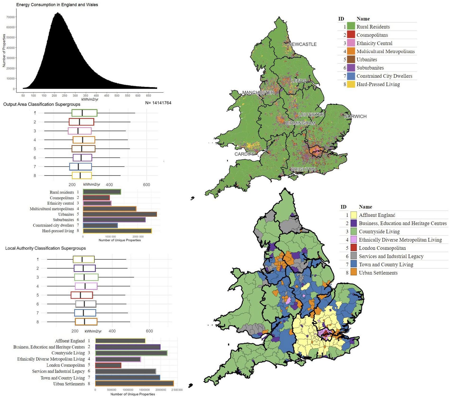
Figure 1. Histogram showing distribution of estimated total energy consumption for the property in a 12 month period (kWh/m²) with breakdowns by OAC and LAC supergroups.

Figure 2

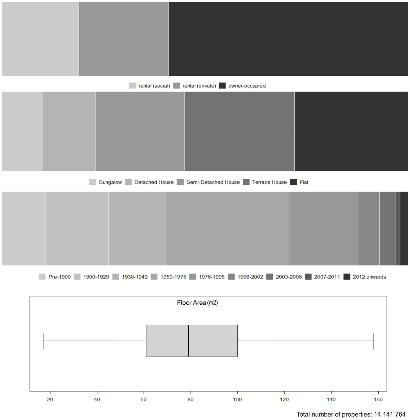
Figure 2. Descriptive statistics of our dwelling sample characteristics.

4.2 Models

Multilevel model for energy consumption per square metre shown in Table 1.

Table 1

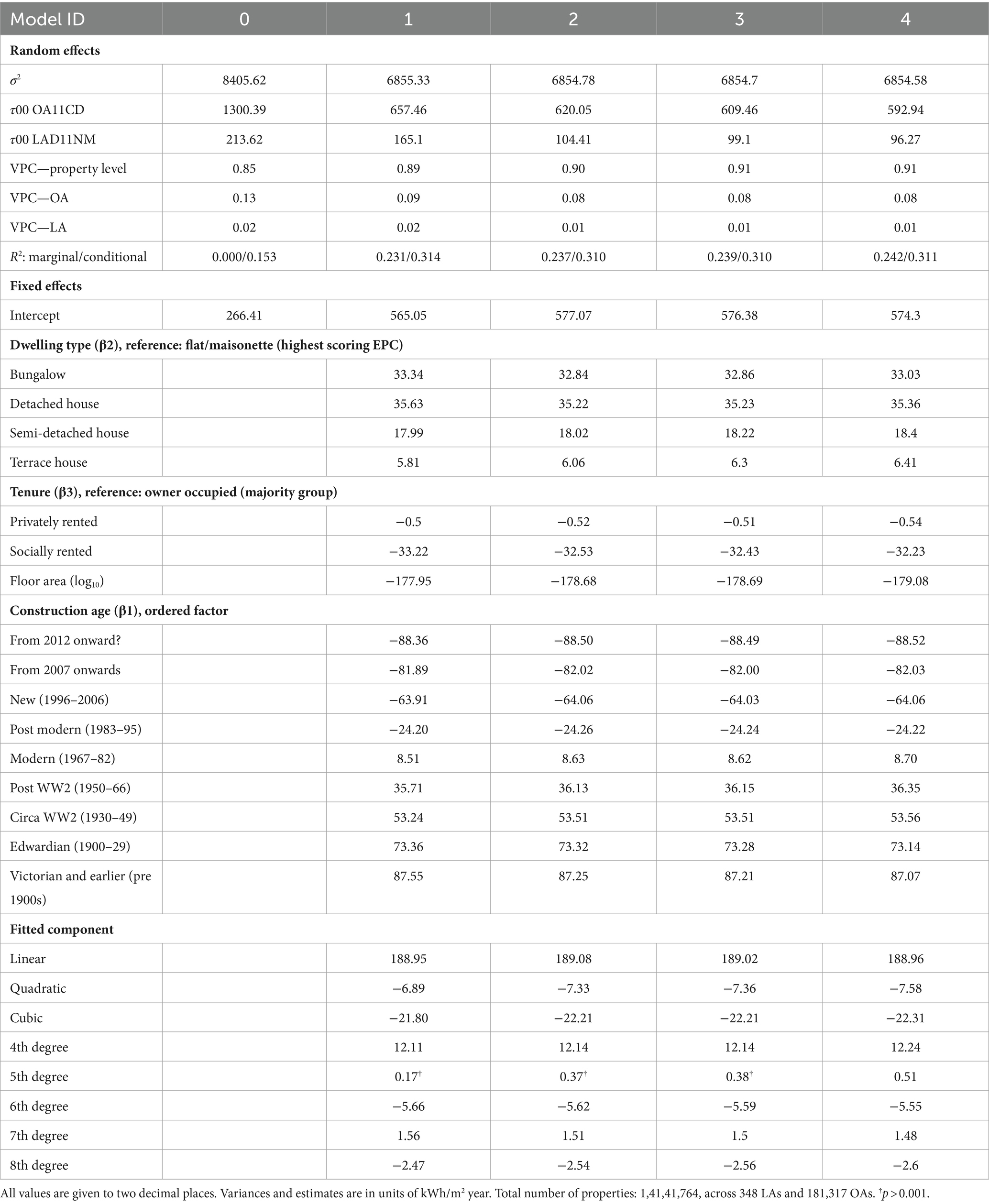
Table 1. Computational notation: multilevel models for energy consumption per square metre.

4.3 Classification fixed effects

Area classification fixed effects of Model 2 shown in Table 2.

Table 2

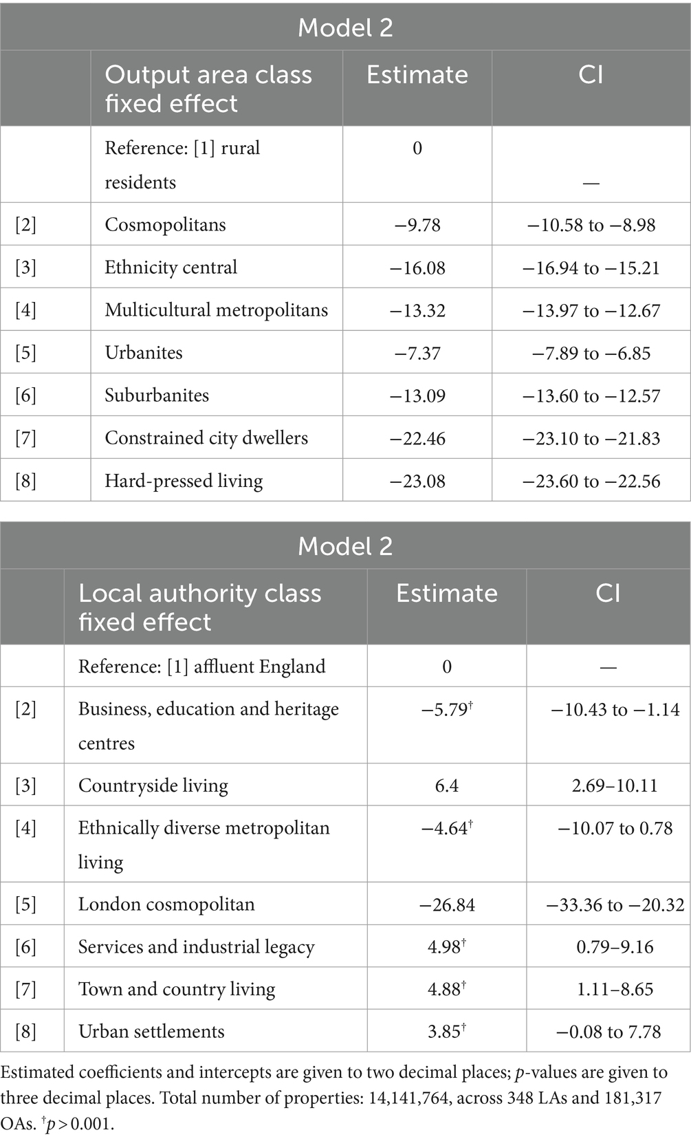
Table 2. Area classification fixed effects of Model 2.

4.4 Output area class fixed effects

Output area classification fixed effects of Model 3 (left) and 4 (right) shown in Figure 3.

Figure 3

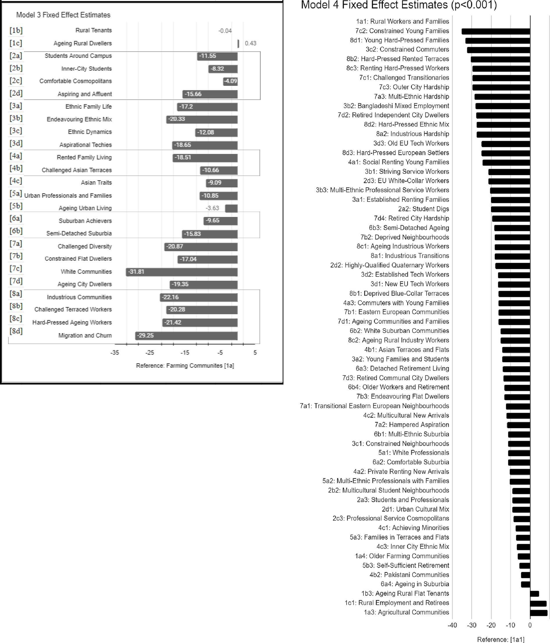
Figure 3. Output area classification fixed effects of Model 3 (left) and 4 (right). Estimated coefficients and intercepts are given to two decimal places; p-values are given to three decimal places.

5 Discussion

5.1 Persistent high variance at the property level

Our descriptive statistics in Figure 1 set the expectation that there is some difference between output area and local authority classes. At the local authority class level, there is negligible difference between groups. Only London cosmopolitans (LAC 5) homes are expected to have slightly lower energy consumption, likely reflecting their over-representation in more energy efficient flats. At a finer scale, we do not observe a strong social gradient. However, these descriptive observations do not control for variance at the property-level, immediate neighbourhood or specific local authority effects.

Model 0 examines the partition of variance in energy performance between three levels: the specific LA level, OA level, and property level. The conditional R² indicates that geographical location alone—as defined by a property’s OA and LA—can explain about 15% of the variance in predicted energy consumption per m². The VPC scores for this model show that the vast majority of this variance (85%) is between individual properties at the lowest level. Of the variance accounted for by the higher levels, much more can be attributed to differences between OAs (13%) than to differences between LAs (2%). This suggests that the at this time, the LA level is of limited value for understanding differences in energy performance, perhaps because local authorities, through local councils, have not yet played the role envisaged for them in the future by central government in delivering net-zero commitments (Rankl et al., 2023). Our observation of only minor differences at LA level is consistent with previous work examining (a lack of) differences in retrofit needs in the UK at this level (Ahlrichs et al., 2022). The high variance at the property level is a reminder of the heterogeneity in housing, even within small neighbourhoods such as output areas.

Model 1 extends Model 0 by adding various property-level characteristics (type, tenure, floor area, and building age). The aim of Model 1 is to determine how much of the variance at each level can be explained by these additional property-level features. All the included property features are significant and these together account for about 23% of the overall variance in the estimated energy consumption per property, as indicated by the marginal R² of Model 1. We also note, as would be expected, that the variances at all three levels previously discussed—specifically LA level, OA level, and property level—have all been substantially reduced, indicating that a considerable proportion of the variance between OAs and LAs was related to the difference mix of properties found in those areas. In addition, Model 1 indicates that the inclusion of property level features increases the proportion of variance explained by the model as a whole from 15% to 31%, based on the conditional R². In other words, much of the variance in energy performance (69%) remains unexplained by any of the features of the model. This variation may be attributed to measurement errors such as inconsistencies in measures between surveyors or biases in the surveys, as discussed earlier in this paper.

5.2 Similarities in privately rented and owner-occupied homes

Taking a closer look at the coefficients of the property-level explanatory variables, we see our results broadly align with previous research. The differences related to age are far greater than those related to type, size or tenure. Newer properties are substantially more efficient (lower energy consumption per square metre), reflecting the increased standards set by Building Regulations over time (Dowson et al., 2012). We also see how properties with fewer external surfaces (flats, then terraced houses, then semi-detached) have higher energy efficiency for reasons of basic physics as they have fewer thermal bridges. Larger properties, likewise, are more efficient (i.e., require less energy per square metre) as volume to surface area ratios increase (but note that the coefficient here is for the log10 of size, so this is showing the effect of making a property 10 times larger).

Private rented properties have been the subject of heavy policy and regulatory focus because of the split incentive issue, where residential upgrades would cost but not directly benefit landlords when only tenants stand to benefit from lower energy consumption bills directly. Supporting this, Petrov and Ryan (2021) find that privately rented properties in Ireland tend to be slightly less efficient than comparable stock. By contrast, data from the ONS suggests a more complex relationship, where new owner-occupied homes are slightly more efficient than their rental counterparts with this reversed for existing dwellings (Bowers et al., 2022, p. 5). We find that once we control for age and type, the energy efficiency of privately rented homes appears to be practically indistinguishable from that of owner-occupied properties (the reference class), with a modelled difference of just −0.5 kWh/m² year. The low average for private renting likely reflects the concentration of the stock in well-connected and established areas, which tend to older, inner urban housing (Bailey et al., 2023) rather than the behaviour of landlords (Miu and Hawkes, 2020), i.e., their failure to invest in energy efficiency measures in the same way as social landlords have. However, because EPCs are only issued at the point of a transaction or in response to some specific upgrade scheme that requires it, some owner-occupied fabric upgrades will not be captured over extensive periods. Socially rented stock is markedly more efficient than either private tenure. This may reflect the more systematic approach to property maintenance and upgrading from large social landlords with a long-term asset management approach as well as regulatory requirements on the sector, for example under the Clean Growth strategy (HM Government, 2019). There may also be a policy factor here as significant efforts have been focussed on this sector through initiatives such as the Decent Homes standard in the early 2000s and, more recently, the Social Housing Decarbonisation Fund (HCLG Committee, 2021).

5.3 Co-occurence of disadvantage and lower energy consumption homes

In Models 2–4, we introduce increasingly fine-grained socio-demographic classifications as fixed effects at OA and LA levels. At the local authority level, the most striking feature is the higher levels of energy efficiency in “London Cosmopolitan,” which really sits apart from the other supergroups. This covers 11 inner London boroughs, including several with high levels of social deprivation and good transport connectivity. One explanation for this might lie in actions by the relevant authorities, but there is little evidence in policy discussions to suggest they have been preferentially funded or more active in relation to this area. An alternative explanation might lie in the London housing market, where the exceptionally high property values may make reinvestment in properties, including works to raise energy efficiency, a more commercially attractive proposition. In addition, the dominant property type in this area will be flats, which for physical reasons already mentioned are more energy efficient.

From the descriptive statistics in Figure 1, we expect, that knowing nothing else, less well-off neighbourhoods, such as those in constrained city dwellers (OAC 7) and ethnicity central (OAC 3) output areas, have a lower estimated residential energy consumption and therefore more energy efficient homes, possibly reflecting concentrations of social housing in these areas. By contrast, rural residents (OAC 1) and metropolitan residents (OAC 4) occupy neighbourhoods with mildly energy-leakier homes. Models 2–4 confirm that even after controlling for property mix, more disadvantaged areas seem to have more efficient housing. Table 2 shows higher energy efficiency is associated with areas of hard-pressed living (OAC 8) or constrained city dwellers (OAC 7), while the lowest are rural residents (OAC 1) then urbanites (OAC 5), and cosmopolitans (OAC 2). Model 3 shows that constrained city dwellers, especially white communities (7c) and hard-pressed living, especially characterised by migration and churn (8d) tend to have the lowest estimated energy consumption on their dwellings, even when controlling for social rent and property age. A closer look at the most energy-efficient homes—i.e. those with the lowest expected energy consumption (e.g., 7c2, 8d1, 3c2 in Figure 3) we see that these tend to be working families. This is interesting and contrasts with previous work by Wenninger et al. (2022), who note that retrofit improvements are less common in areas with high concentrations of families with children under 15.

At the output area level, we can think of the systematic differences as arising from two processes: the selection of different kinds of housing by different social groups; and differential abilities or interests in improving energy efficiency between social groups. Our main finding is that we see little evidence that more affluent groups are preferentially selecting more efficient properties or that they are taking action at higher rates—quite the opposite. One policy factor which may underlie this finding is that many of the national energy efficiency programmes have been targeted wholly or in part at more disadvantaged groups, including low-income households and households containing a person with disabilities, and we would expect high concentrations of both groups in the hard-pressed living (OAC 8) and constrained city dwellers (OAC 7) areas.

5.4 Energy efficiency drivers: hidden at the finest scales

Since the classification features are associated with the higher levels of Model 1, they cannot meaningfully improve its explanatory power, as modelled by the conditional R². Instead, they could explain variance that was attributed to the OA and LA level random effects in the previous models. If the classifications were strongly associated with energy performance, after controlling for our other variables, we would expect to see substantial reductions in the variances reported at the OA and LA levels (as compared with Model 1), decreases in the OA and LA level VPCs and an increase in the marginal R². We would also expect these changes to be greater for the models with more classes since these have the capacity to explain more of the higher-level variance.

While we do observe changes of this nature, their scale is limited. Variance at OA level drops from 657 in Model 1 (without classifications), to 620 in Model 2 (highest level classifications), through to 593 in Model 4 (lowest level, i.e., most granular classifications), while the variance at LA level drops from 165 in Model 1, to 104 in Model 2, through to 96 in Model 3. The drop in variance at LA level is clearly proportionally much greater, but the overall proportion of variance associated with this level is so low that the practical significance of any observations at this scale is questionable. Marginal R² increases from 23.1% for Model 1, to 23.7% for Model 2, through to 24.2% for Model 4, suggesting that OA and LA classifications, even at the most detailed level, can explain only just over 1% of the overall variance in predicted energy consumption per m². Using finer-grained area classifications (the groups and sub-groups of Models 3 and 4) does not do a great deal to increase explanatory power in the fixed part of the models. The bulk of unexplained variance remains at the property level. This aligns with previous work that had found socio-demographic characteristics less potent than dwelling-related characteristics for capturing retrofit investments that would lower a home’s energy consumption (Trotta, 2018).

Two broad conclusions can be drawn here. Firstly, while geography—at least, down to the scale of output areas—explains some of the variance in EPC rating, a majority of the variance is unexplained. This implies that other differences between individual properties are responsible for the majority of variation in energy efficiency. Secondly, the proportion of variance in estimated energy consumption per m² that is explained by geography, is mostly at the finer scale of OAs, rather than the larger scale of LAs. In other words, there is very little large geographic scale variation in EPC ratings across England and Wales; the largest part of geographic variations are at a much finer neighbourhood-to-neighbourhood, street-to-street or even property-to-property level.

6 Conclusion

Our analysis produces three main conclusions. First, at the highest geographic scale, residential energy efficiency varies comparatively little between local authorities. All face broadly similar challenges. This is perhaps surprising given that local authorities have been given a central role for coordinating efforts in this area for some time (Morris et al., 2017) thus we might expect a degree of divergence. The fact that our work cannot show evidence of this is perhaps indicative of the enormous constraints on local government which have arisen from years of austerity (Hastings et al., 2017; Morris et al., 2017). The House of Commons HCLG Committee (2021) recently called for greater use of local authorities within the national retrofit policy but this is unlikely to prove successful unless these basic resource constraints are addressed.

Second, at the neighbourhood scale, we do not see strong relationships between the social composition or socio-economic status of neighbourhoods (output areas) and energy efficiency, contrary to what we might have expected. Despite extensive coverage of the climate crisis in general and some discussion of domestic energy efficiency issues in particular, it appears that more socially advantaged groups are not choosing or able to use their resources to achieve more sustainable housing. Possible explanations can be found in recent qualitative research in Scotland on homeowner attitudes to this issue (Energy Savings Trust and Taylor McKenzie, 2023). This reveals a striking “disconnect” in homeowner thinking (p2): on the one hand, a general awareness of and support for the “net zero” goal but, on the other, limited awareness of what this might mean for them or any sense that they were responsible for acting in relation to their own homes. Barriers cited by homeowners included costs but also a sense that, without “a clear, personal financial benefit from upgrading,” it was for Government or business to lead the way. Policy may be quite correctly targeting initial support on the more disadvantaged or vulnerable groups but more will clearly need to be done to encourage, enable and/or require those with greater means to apply these to their own energy efficiency if we are to meet “net zero” targets. Despite the lack of strong variations at a neighbourhood level, small area targeting may still have an important role to play. Other justifications include the possible reduced coordination costs from concentrating interventions, the gains in owner motivation from seeing neighbours taking action and the supply chain benefits of concentrated demand reducing costs and increasing trust. Localised action can also work effectively with support services such as “One Stop Shops” to support action by owners (Bertoldi et al., 2021a,b).

Given owners’ focus on the financial returns of energy efficiency, one important area for research would be to provide evidence on the scale of any such returns. The key questions for future research in this direction would include: whether there is evidence that energy efficiency is becoming more important over time as debates about pathways to net zero become more prominent; whether this matters more in home purchase decisions or renting; and whether it is energy cost measures or carbon emissions which weigh most in consumer valuations of properties. Further research is also required to ascertain whether carrot or stick incentives may affect changes in attitude more readily. In the UK context, linking taxes such as stamp duty (paid when purchasing property) to energy efficiency with significantly lower rates for more efficient properties, might incentivise sellers to improve their properties before sale. Alternative progressive taxes associated, for example, with Council Tax, could be further imagined, as well as mortgage or borrowing benefits for energy efficient upgrades.

Third, our work produces a novel finding in relation to housing tenure. Once we allow for the fact that private landlords tend to own smaller, older properties, the energy efficiency levels reported appear no lower than those for owner-occupiers. With the minor caveat that tenure is only recorded at the time of the survey, we do not observe a particular energy efficiency problem with private renting. There has been much discussion of the reasons why private landlords may be less likely to invest in energy efficiency since it is tenants rather than landlords who get the direct benefit from improvements in terms of lower bills. However, our data do not support the underlying premise that energy efficiency is therefore lower in the private rented sector. This policy focus on private renting can possibly be justified in other ways. For example, the Scottish Government’s (2023) proposals to set an earlier deadline for private landlords to meet a new energy efficiency standard is justified in part by reference to higher levels of fuel poverty in the sector. As it stands, however, our finding suggests less need to focus efforts specifically by tenure and rather more need to encourage, enable or require private owners to make the necessary changes across the board.

Data availability statement

Publicly available datasets were analyzed in this study. This data can be found here: https://epc.opendatacommunities.org/.

Author contributions

BB: Conceptualization, Data curation, Formal analysis, Investigation, Methodology, Project administration, Resources, Software, Visualization, Writing – original draft, Writing – review & editing. TO-E: Conceptualization, Formal analysis, Methodology, Validation, Writing – original draft, Writing – review & editing. NB: Conceptualization, Data curation, Formal analysis, Funding acquisition, Methodology, Supervision, Writing – original draft, Writing – review & editing. AD: Conceptualization, Funding acquisition, Project administration, Resources, Writing – review & editing, Writing – original draft.

Funding

The author(s) declare financial support was received for the research, authorship, and/or publication of this article. We would like acknowledge support from the Ordnance Survey, which made the foundations of this research possible and UCL Library Services who enabled the open-sourcing of this manuscript. BB is a Co-Investigator on ESRC’s funding for the International Public Policy Observatory’s local data research stream [ES/X008282/1] and NB’s involvement was enabled by the ESRC’s ongoing support for the Urban Big Data Centre (UBDC) (ES/L011921/1 and ES/S007105/1).

Conflict of interest

The authors declare that the research was conducted in the absence of any commercial or financial relationships that could be construed as a potential conflict of interest.

Publisher’s note

All claims expressed in this article are solely those of the authors and do not necessarily represent those of their affiliated organizations, or those of the publisher, the editors and the reviewers. Any product that may be evaluated in this article, or claim that may be made by its manufacturer, is not guaranteed or endorsed by the publisher.

References

Ahlrichs, J., Wenninger, S., Wiethe, C., and Häckel, B. (2022). Impact of socio-economic factors on local energetic retrofitting needs—a data analytics approach. Energy Policy 160:112646. doi: 10.1016/j.enpol.2021.112646

Crossref Full Text | Google Scholar

Bailey, N., and Gannon, M. (2018). More similarities than differences: poverty and social exclusion in rural and urban populations, in Poverty and social exclusion in the UK: volume 1 - the nature and extent of the problem, (Eds.) E. Dermott and G Main. (Bristol: Policy Press), 223–242.

Google Scholar

Bailey, N., Livingston, M., and Chi, B. (2023). Housing and welfare reform, and the suburbanisation of poverty in UK cities 2011-20, Housing Studies. doi: 10.1080/02673037.2023.226639

Crossref Full Text | Google Scholar

Beillan, V., Battaglini, E., Goater, A., Ines Mayer, A. H., and Trotignon, R. (2011). Barriers and drivers to energy-efficient renovation in the residential sector. Empirical findings from five European countries : ECEEE Available at: https://www.eceee.org/library/conference_proceedings/eceee_Summer_Studies/2011/5-saving-energy-in-buildings-the-time-to-act-is-now/barriers-and-drivers-to-energy-efficient-renovation-in-the-residential-sector-empirical-findings-from-five-european-countries/.

Google Scholar

BEIS (2021). Net zero strategy: build back greener. London: Department for Business, Energy & Industrial Strategy. Available at: https://www.gov.uk/government/publications/net-zero-strategy

Google Scholar

Bergman, N., and Foxon, T. J. (2020). Reframing policy for the energy efficiency challenge: insights from housing retrofits in the United Kingdom. Energy Res. Soc. Sci. 63:101386. doi: 10.1016/j.erss.2019.101386

Crossref Full Text | Google Scholar

Bertoldi, P., Boza-Kiss, B., Della Valle, N., and Economidou, M. (2021a). The role of one-stop shops in energy renovation—a comparative analysis of OSSs cases in Europe. Energy Build. 250:111273. doi: 10.1016/j.enbuild.2021.111273

Crossref Full Text | Google Scholar

Bertoldi, P., Economidou, M., Palermo, V., Boza-Kiss, B., and Todeschi, V. (2021b). How to finance energy renovation of residential buildings: review of current and emerging financing instruments in the EU. WIREs Energy Environ. 10:e384. doi: 10.1002/wene.384

Crossref Full Text | Google Scholar

Bowers, N., Smith, C., and Wilkins, T. (2022). Energy efficiency of housing in England and Wales—Office for National Statistics : Office for National Statistics Available at: https://www.ons.gov.uk/peoplepopulationandcommunity/housing/articles/energyefficiencyofhousinginenglandandwales/2022.

Google Scholar

Brito, N. (2023). “Improving the (energy) performance of (historic) buildings and communities: towards “neighbourhood energy performance certification” (nEPC)” in EEHB 2022 post prints (Stuttgart: Fraunhofer IRB Verlag), 73–80.

Google Scholar

Brounen, D., Kok, N., and Quigley, J. M. (2012). Residential energy use and conservation: economics and demographics. Eur. Econ. Rev. 56, 931–945. doi: 10.1016/j.euroecorev.2012.02.007

Crossref Full Text | Google Scholar

Buyuklieva, B., Dennett, A., Bailey, N., and Morley, J. (2023). Energy efficient homes: the social and spatial patterns of residential energy efficiency in England. arXiv. Available at: https://doi.org/10.48550/arXiv.2302.09628. [Epub ahead of preprint].

Google Scholar

Chaudhuri, K., and Huaccha, G. (2023). Who bears the energy cost? Local income deprivation and the household energy efficiency gap. Energy Econ. 127:107062. doi: 10.1016/j.eneco.2023.107062

Crossref Full Text | Google Scholar

Comerford, D. A., Moro, M., Sejas-Portillo, R., and Stowasser, T. (2021). Leveraging the motivational effects of labels: lessons from retrofitting. Behav. Sci. Policy 7, 17–25. doi: 10.1177/237946152100700203

Crossref Full Text | Google Scholar

Corcoran, J., Higgs, G., and Anderson, T. (2013). Examining the use of a geodemographic classification in an exploratory analysis of variations in fire incidence in South Wales, UK. Fire Saf. J. 62, 37–48. doi: 10.1016/j.firesaf.2013.03.004

Crossref Full Text | Google Scholar

Crawley, J., Biddulph, P., Northrop, P. J., Wingfield, J., Oreszczyn, T., and Elwell, C. (2019). Quantifying the measurement error on England and Wales EPC ratings. Energies 12:3523. doi: 10.3390/en12183523

Crossref Full Text | Google Scholar

DECC (2014). Green deal assessment mystery shopping research: mystery shopping of customer experiences of green deal assessments with 48 households and analysis of variability across green deal assessment reports of 29 properties : Department of Energy and Climate Change Available at: https://assets.publishing.service.gov.uk/government/uploads/system/uploads/attachment_data/file/388197/Green_Deal_Assessment_Mystery_Shopping_FINAL_PUBLISHED.pdf.

Google Scholar

Dennett, A., and Stillwell, J. (2009). Internal migration in Britain, 2000–01, examined through an area classification framework. Popul. Space Place 16:517. doi: 10.1002/psp.554

Crossref Full Text | Google Scholar

DLUHC (2023). Dwelling stock estimates, England: 31 March 2022. Available at: https://www.gov.uk/government/statistics/dwelling-stock-estimates-in-england-2022/dwelling-stock-estimates-england-31-march-2022

Google Scholar

Dowson, M., Poole, A., Harrison, D., and Susman, G. (2012). Domestic UK retrofit challenge: barriers, incentives and current performance leading into the green deal. Energy Policy 50, 294–305. doi: 10.1016/j.enpol.2012.07.019

Crossref Full Text | Google Scholar

Druckman, A., and Jackson, T. (2008). Household energy consumption in the UK: a highly geographically and socio-economically disaggregated model. Energy Policy 36, 3177–3192. doi: 10.1016/j.enpol.2008.03.021

Crossref Full Text | Google Scholar

Energy Savings Trust and Taylor McKenzie (2023). Qualitative research into domestic property owners’ attitudes to net zero heating and energy efficiency standards : Scottish Government.

Google Scholar

Few, J., Manouseli, D., McKenna, E., Pullinger, M., Zapata-Webborn, E., Elam, S., et al. (2023). The over-prediction of energy use by EPCs in Great Britain: a comparison of EPC-modelled and metered primary energy use intensity. Energy Build. 288:113024. doi: 10.1016/j.enbuild.2023.113024

Crossref Full Text | Google Scholar

Gale, C. G., Singleton, A. D., Bates, A. G., and Longley, P. A. (2016). Creating the 2011 area classification for output areas (2011 OAC). J. Spat. Inf. Sci. 12:232. doi: 10.5311/JOSIS.2016.12.232

Crossref Full Text | Google Scholar

Gazze, L. (2023). Achieving net zero goals in residential buildings. J. Br. Acad. 11s4, 35–56. doi: 10.5871/jba/011s4.035

Crossref Full Text | Google Scholar

Geospatial Commission (2020). Unlocking the power of location: The UK’s geospatial strategy 2020 to 2025. Available at: https://www.gov.uk/government/publications/unlocking-the-power-of-locationthe-uks-geospatial-strategy/unlocking-the-power-of-location-the-uks-geospatial-strategy-2020-to-2025

Google Scholar

Gledhill, T., Swan, W., and Fitton, R. (2023). A practitioner study into the variability of UK domestic energy assessments. Int. J. Build. Pathol. Adapt. doi: 10.1108/IJBPA-10-2022-0167

Crossref Full Text | Google Scholar

Gupta, R., and Gregg, M. (2018). Targeting and modelling urban energy retrofits using a city-scale energy mapping approach. J. Clean. Prod. 174, 401–412. doi: 10.1016/j.jclepro.2017.10.262

Crossref Full Text | Google Scholar

Hastings, A., Bailey, N., Bramley, G., and Gannon, M. (2017). Austerity urbanism in the UK: the regressive redistribution of local government services, and the impact on the poor and marginalised in English cities. Environ. Plan. A 49, 2007–2024. doi: 10.1177/0308518X17714797

Crossref Full Text | Google Scholar

HCLG Committee (2021). Local government and the path to net zero. London Available at: https://committees.parliament.uk/publications/7690/documents/80183/default/

Google Scholar

HM Government (2019) Leading on clean growth: the government response to the committee on climate change’s 2019 progress report to parliament—reducing UK emissions. London: HM Government.

Google Scholar

BRE Housing (2008). Part I: Dwelling and Household Characteristics of Hard To Treat Homes. Available at: https://files.bregroup.com/bre-co-uk-file-library-copy/filelibrary/pdf/rpts/Hard_to_Treat_Homes_Part_I.pdf

Google Scholar

Huaccha, G. (2023). Regional persistence of the energy efficiency gap: evidence from England and Wales. Energy Econ. 127:107042. doi: 10.1016/j.eneco.2023.107042

Crossref Full Text | Google Scholar

Hurst, L. J., and O’Donovan, T. S. (2019). A review of the limitations of life cycle energy analysis for the design of fabric first low-energy domestic retrofits. Energy Build. 203:109447. doi: 10.1016/j.enbuild.2019.109447

Crossref Full Text | Google Scholar

Mallaburn, P. S., and Eyre, N. (2014). Lessons from energy efficiency policy and programmes in the UK from 1973 to 2013. Energy Effic. 7, 23–41. doi: 10.1007/s12053-013-9197-7

Crossref Full Text | Google Scholar

McMichael, M., and Shipworth, D. (2013). The value of social networks in the diffusion of energy-efficiency innovations in UK households. Energy Policy 53, 159–168. doi: 10.1016/j.enpol.2012.10.039

Crossref Full Text | Google Scholar

Miu, L., and Hawkes, A. D. (2020). Private landlords and energy efficiency: evidence for policymakers from a large-scale study in the United Kingdom. Energy Policy 142:111446. doi: 10.1016/j.enpol.2020.111446

Crossref Full Text | Google Scholar

Moon, G., Twigg, L., Jones, K., Aitken, G., and Taylor, J. (2019). The utility of geodemographic indicators in small area estimates of limiting long-term illness. Soc. Sci. Med. 227, 47–55. doi: 10.1016/j.socscimed.2018.06.029

PubMed Abstract | Crossref Full Text | Google Scholar

Morris, J., Harrison, J., Genovese, A., Goucher, L., and Koh, S. C. L. (2017). Energy policy under austerity localism: what role for local authorities? Local Gov. Stud. 43, 882–902. doi: 10.1080/03003930.2017.1359164

Crossref Full Text | Google Scholar

Nakagawa, S., and Schielzeth, H. (2013). A general and simple method for obtaining R² from generalized linear mixed-effects models. Methods Ecol. Evol. 4, 133–142. doi: 10.1111/j.2041-210x.2012.00261.x

Crossref Full Text | Google Scholar

ONS (2018). Methodology and variables : Office for National Statistics Available at: https://www.ons.gov.uk/methodology/geography/geographicalproducts/areaclassifications/2011areaclassifications/methodologyandvariables.

Google Scholar

Owen, A., Middlemiss, L., Brown, D., Davis, M., Hall, S., Bookbinder, R., et al. (2023). Who applies for energy grants? Energy Res. Soc. Sci. 101:103123. doi: 10.1016/j.erss.2023.103123

Crossref Full Text | Google Scholar

Petrov, I., and Ryan, L. (2021). The landlord-tenant problem and energy efficiency in the residential rental market. Energy Policy 157:112458. doi: 10.1016/j.enpol.2021.112458

Crossref Full Text | Google Scholar

Piao, X., and Managi, S. (2023). Household energy-saving behavior, its consumption, and life satisfaction in 37 countries. Sci. Rep. 13:1382. doi: 10.1038/s41598-023-28368-8

PubMed Abstract | Crossref Full Text | Google Scholar

Rankl, F., Collins, A., Tyers, R., and Carver, D. (2023). The role of local government in delivering net zero : House of Commons Library Available at: https://commonslibrary.parliament.uk/research-briefings/cdp-2023-0122/.

Google Scholar

Robinson, C., Lindley, S., and Bouzarovski, S. (2019). The spatially varying components of vulnerability to energy poverty. Ann. Am. Assoc. Geogr. 109, 1188–1207. doi: 10.1080/24694452.2018.1562872

Crossref Full Text | Google Scholar

Scottish Government (2023) Delivering net zero for Scotland’s buildings: a consultation on proposals for a heat in buildings bill. Edinburgh: Scottish Government.

Google Scholar

Tingey, M., and Webb, J. (2020). Governance institutions and prospects for local energy innovation: laggards and leaders among UK local authorities. Energy Policy 138:111211. doi: 10.1016/j.enpol.2019.111211

Crossref Full Text | Google Scholar

Trotta, G. (2018). The determinants of energy efficient retrofit investments in the English residential sector. Energy Policy 120, 175–182. doi: 10.1016/j.enpol.2018.05.024

Crossref Full Text | Google Scholar

UCLA: Statistical Consulting Group. R library contrast coding systems for categorical variables. Available at: https://stats.oarc.ucla.edu/r/library/r-library-contrast-coding-systems-for-categorical-variables/

Google Scholar

Watson, P. (2010). An introduction to UK energy performance certificates (EPCs). J. Build. Apprais. 5, 241–250. doi: 10.1057/jba.2009.22

Crossref Full Text | Google Scholar

Wenninger, S., Karnebogen, P., Lehmann, S., Menzinger, T., and Reckstadt, M. (2022). Evidence for residential building retrofitting practices using explainable AI and socio-demographic data. Energy Rep. 8, 13514–13528. doi: 10.1016/j.egyr.2022.10.060

Crossref Full Text | Google Scholar

Appendix

Output Area Classifications

At the finest-grained geographic scale, the UK Office for National Statistics (ONS) output area classification (OAC) The latest iteration of OAC was released after and based on data from the 2011 Census. These dimensions fall broadly into five domains: demographic structure, household composition, housing, socio-economic and employment; or, for our purposesṣ—three types: socio-demographic (including concentrations of groups based on age, household types, ethnicity and location birth categories), education and employment (including qualification types and employment industries), and residential setup (including commute type, car ownership and housing information such as tenure and property type). The OAC can be used to think about the energy efficiency of homes in different neighbourhoods by enabling clusters of dwellings to be grouped according to similar types of local characteristics.

Local Authority

The output area classification assigns small geographic areas into distinct groups based on socio-economic and demographic attributes, allowing for granular insights into localised characteristics. On the other hand, the local authority area classification groups larger administrative areas to uncover broader patterns across municipalities. The classifications each consist of three levels, each nested within the other. At higher levels of spatial granularity, such as at the local authority level, area classifications can be useful for contextualising the overall patterns observed at the policy levels. Specifically, the output areas and their classification can serve as the lower level, capturing localised variations, while the local authorities and their area classification can act as the higher level, encompassing broader planning or sub-regional trends.

Table 1

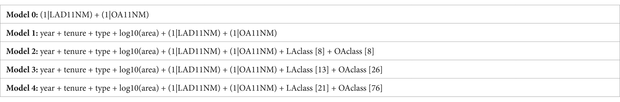
Table 1. Multilevel model for energy consumption per square metre.