Model-based monocular 6-degree-of-freedom pose tracking for asteroid

In this paper, we present a novel vision-based framework to track the 6-DoF pose of an asteroid in real time with the 3D contour of the asteroid as a feature. During pose tracking, at the beginning time of tracking, the tracking system is initialized by a pose retrieval method. At each subsequent time instant, given the 3D mesh model of an asteroid, with the initial pose and its covariance given by the square root cubature Kalman Filter (SCKF), the 3D mesh segments constituting the 3D asteroid contour are efficiently extracted from the 3D mesh model. Then, in the input asteroid image, we search the image points corresponding to the extracted 3D segments within the searching range defined by the initial pose and its covariance. After that, the asteroid pose is determined in real time by minimizing the angles between the back-projection lines of the searched image points and the projection planes of the corresponding 3D segments, which is much more robust to the position change of the asteroid and asteroid size. The covariance matrix of the pose is inferred from the Cartesian noise model in the first order. Eventually, the SCKF is derived from the second-order auto regression to generate the final pose estimate and give the initial pose and its covariance for the next time instant. The synthetic trials quantitatively validate the real-time performance, robustness, and accuracy of our algorithm in dark space, different imaging distances, lighting conditions, image noise, model error, and initial pose error, and meanwhile, the real trial qualitatively shows the effectiveness of our method.

1 Introduction

Asteroid exploration plays a fundamental role in many space missions, such as deep space navigation and autonomous landing (Watanabe et al., 2017; Sugita et al., 2019; Golish et al., 2020). It is essential for asteroid exploration to accurately determine the 6-degrees-of-freedom (DoF) pose in real time. In recent decades, monocular 6-DoF pose tracking has become increasingly significant and widely used in many space missions, such as landing, docking, and rendezvous, thanks to its accuracy, speed, low energy cost, and cheapness (Kelsey et al., 2006; Forshaw et al., 2016; Opromolla et al., 2017; Huo et al., 2020; Huang et al., 2021a). However, it is still challenging to apply the monocular 6-DoF pose tracking method to asteroids due to the highly irregular shape of asteroids and dramatic illuminance variation.

In general, monocular 6-DoF pose tracking methods rely on feature point matching, machine learning, region segmentation, and edge alignment. The feature-point-based methods predefine some remarkable 3D feature points on the target 3D model a priori and then match the 3D feature points against the corresponding image points. The pose is solved from the 2D-3D matching by the Perspective-n-Point (PnP) algorithm (Huo et al., 2020; Conway et al.; Hu et al., 2021; Black et al., 2021; Leroy et al., 2001; Capuano et al., 2020; Chen et al., 2019; Huang et al., 2021b; Stacey and D’Amico, 2018; Liu and Hu, 2014; Peng et al., 2020; Crivellaro et al., 2017; Meng et al., 2018; Rowell et al., 2015; Long and Hu, 2022; Liu et al., 2020a; Christian, 2015; Li and Xu, 2018; Cassinis et al., 2022). However, it is difficult to specify sufficient remarkable 3D feature points on an asteroid since it is irregular and textureless (Huang et al., 2020). Machine learning-based methods use some labeled images to train a mapping from the image space to pose space a priori, via convolution neural network (Rathinam et al., 2022; Sharma et al., 2018; Sharma and D’Amico, 2020; Zhou et al., 2021), image regression (Raytchev et al., 2011; Cao et al., 2016), and similarity measurement (Zhang et al., 2018). During pose determination, the trained system immediately provides a pose estimate to asteroids according to the input image (Kelsey et al., 2006; Liu et al., 2020a; Christian, 2015; Li and Xu, 2018; Rathinam et al., 2022; Sharma et al., 2018; Sharma and D’Amico, 2020; Cao et al., 2016; Raytchev et al., 2011; Zhang et al., 2018; Zhou et al., 2021; Sattler et al., 2019; Rondao et al., 2021; Pugliatti and Topputo, 2022; He et al., 2020). For accuracy, such a method requires considerable labeled image samples and the sample space should cover the real work range (Sattler et al., 2019). In fact, it is difficult to obtain many labeled real images of asteroids. Furthermore, since the asteroid tumbles in deep space, the asteroid image is largely related to the viewpoint, illumination condition, and motion, which makes it difficult to build a precise mapping between image space and 6-DoF pose space. The region-based methods first employ a specific color segmentation model to construct an energy function based on posterior probability and then solve the pose from the best consistency of energy functions of silhouette and rendering of the CAD model (Brox et al., 2005; Bray et al., 2006; Dambreville et al., 2008; Prisacariu et al., 2012; Prisacariu and Reid, 2012; Hexner and Hagege, 2016; Tjaden and Schomer, 2017; Zhong et al., 2020; Stoiber et al., 2022). They can deal with pose tracking under cluttered backgrounds and motion blur properly (Stoiber et al., 2022). However, they require a large interframe intersection of the foreground for accuracy (Wang et al., 2023) and are not suitable for heterogeneous configurations (both foreground and background) and partial occlusions (Zhong et al., 2020). Therefore, they are incapable of estimating the pose of asteroids in deep space since a large area of self-occlusion may occur on asteroids due to complicated illumination. In addition, frequent rendering makes real-time implementation impossible. The edge-based methods acquire the pose by aligning the edge of the rendered CAD model with the image edges (Petit et al., 2012a; Petit et al., 2012b; Kanani et al., 2012; Oumer et al., 2015; Lourakis and Zabulis, 2017; Marchand et al., 2019; Liu et al., 2020b; Comellini et al., 2020; Huang et al., 2020; Lentaris et al., 2020). These methods are accurate and robust in complex illumination conditions and particularly suitable for smooth and poorly textured targets. However, they lack robustness to the noise and cluttered background, and rendering the CAD model will be time-consuming. Liu et al. (2020b) track the 6-DoF pose of asteroids in real time by minimizing the reprojection errors of the 3D contour of the asteroid, without rendering the CAD model of the asteroid. Despite the accuracy and efficiency, these methods are relatively susceptible to the position change of asteroids.

Unlike manufactured objects, asteroids are irregular, lacking geometric structure and trackable features. The 3D contour of the asteroid yields the asteroid silhouette in the image, which describes the external outline of the asteroid in the image. Therefore, the 3D contour is the most remarkable and reliable feature on asteroids and is quite robust against lighting variation, self-occlusion, and viewpoint changes. Accordingly, we propose a novel framework to track the 6-DoF pose in real time with the 3D contour of the asteroid. Given the 3D mesh model of an asteroid, at each tracking instant, the 3D mesh segments constituting the 3D asteroid contour are automatically extracted from the asteroid mesh model. After retrieving the 2D edge points corresponding to extracted 3D segments from the input asteroid image, we determine the asteroid pose in real time by minimizing the angles between the back-projection lines of the retrieved 2D edge points and the projection planes of the corresponding 3D segments (the plane spanned by a 3D segment with camera optical center). After that, the covariance of the pose is inferred in the first order. Based on this, the 2-order auto regression-based (2nd-AR) SCKF is exploited to provide the final unbiased estimate to pose and predict the pose for the next instant. The pipeline of our method will be elaborated on in Section 2. The proposed method exploits the image edge information to track the asteroid’s pose. However, compared to the existing edge-based methods, our method does not render the CAD model, thus it is quite efficient. Furthermore, compared with the existing method using 2D reprojections, our method determines the pose of asteroids by minimizing the line-to-plane angles, which is much more robust to the size of asteroids and position change (Hu et al., 2021). This paper is a great extension of our previous work (Liu et al., 2020b), but the methodology in this paper is completely new: 1) we propose a robust 2D-3D correspondence method based on the covariance of the pose, 2) we determine the asteroid pose by minimizing the angles between the projection planes of the extracted 3D contour segments and the back-projection lines of the corresponding 2D edge points, 3) we infer the covariance matrix of the estimated pose based on the first-order optimality of the pose optimization, and 4) we use 2nd-AR-based SCKF to give the final pose estimate and initialize the pose tracking at the next time instant.

The rest of this paper is structured as follows. Section 2 introduces the overview of our proposed method. Section 3 focuses on the asteroid motion model used in this paper. Section 4 presents the extraction of 3D contour segments and finds the image data correspondence. Section 5 discusses the pose determination in detail. Section 6 infers the covariance matrix of the pose in the first order. Section 7 provides the final pose estimate by 2nd-AR-based SCKF. Section 8 evaluates the performance of the proposed method. Finally, Section 9 draws a conclusion.

2 Algorithm overview

The proposed algorithm tracks the 6-DoF pose of an asteroid in real time by aligning the silhouette of the asteroid with the projected 3D contour of the asteroid. The pipeline of the pose tracking system is showcased in Figure 1, where k denotes the time instant, I_k is an asteroid image taken by a calibrated camera, and p_k is the estimated pose at the time instant of k. At the beginning of tracking (k = 0), the tracking system is initialized by the pose retrieval method proposed in (Liu et al., 2020b). This paper is focused on the real-time 6-DoF pose tracking of asteroids, so the pose initialization strategy is beyond the research scope of this paper. It is noteworthy that there exist other methods available for the initialization (He et al., 2020; Kobayashi et al., 2015; Phisannupawong et al., 2020; Sonawani et al., 2020; Park and D’Amico, 2023; Proença and Gao, 2020). Given the 3D mesh model of the asteroid, at the time instant of k > 0, with the initial pose p_k⁰ and its covariance S_k⁰ provided by the SCKF (see Section 7), the 3D mesh segments that construct the 3D contour of the asteroid are rapidly extracted from the asteroid mesh model (see Section 4.1). Next, we search in I_k the 2D edge points corresponding to the extracted 3D mesh segments within the searching range defined by p_k⁰ and S_k⁰ (see Section 4.2) and then calculate the asteroid pose in real time by minimizing the angles between the back-projection lines of the searched 2D edge points and the projection planes of the corresponding 3D segments with M-estimation (see Section 5). Subsequently, the covariance of the pose is estimated via the first-order optimality condition of the pose minimization (see Section 6). Eventually, based on this covariance, the 2nd-AR-based SCKF generates the final pose estimate p_k and, meanwhile, predicts the pose p_k+1⁰ and its covariance S_k+1⁰ for the next time instant k+1 (see Section 7). In the following section, we will elaborate on our work according to the pipeline shown in Figure 1.

FIGURE 1

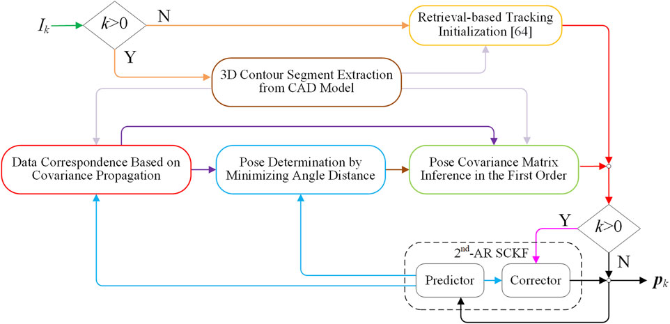
FIGURE 1. Pipeline of our proposed tracking method.

3 Motion representation

This section will introduce the relative pose representation based on the camera modeled by the pinhole. On the asteroid, there is an asteroid coordinate system (ACS). Given the camera intrinsic matrix K, the image x of a 3D point X in ACS can be calculated via Eq. 1

$\stackrel{\sim }{\mathit{x}}\stackrel{\sim }{=}\mathit{K}\left[\begin{array}{cc}\mathit{R}& \mathit{t}\end{array}\right]\stackrel{\sim }{\mathit{X}},(1)$

where $\cong$ denotes the equality up to a scalar; $\stackrel{\sim }{\mathit{X}}$ and $\stackrel{\sim }{\mathit{x}}$ are the homogeneous coordinate vectors of X and x, respectively; R and t denote the rotation matrix and translation vector of ACS to the camera coordinate system (CCS). We adopt Lie group and Lie algebra in SO(3) to formulate the rigid motion of asteroids in the homogeneous coordinate system since it can represent the motion conveniently and without ambiguity. The rotation matrix R is derived from the rotation vector Ω in SO(3) using the Rodrigues formula

$\mathit{R}={\mathit{I}}_3+\frac{\sin ‖\mathit{\Omega }‖{\left[\mathit{\Omega }\right]}_x}{‖\mathit{\Omega }‖}+\frac{\left(1-\cos ‖\mathit{\Omega }‖\right){{\left[\mathit{\Omega }\right]}_x}^2}{{‖\mathit{\Omega }‖}^2},(2)$

where I₃ is the 3-order identity, and [Ω]_x denotes the skew-symmetric matrix formed by the components of Ω. Accordingly, the pose is represented by p = [Ω^T t^T]^T. It can be readily known from Eq. 2 that Ω can be recovered from R via Eq. 3

$\begin{array}{l}‖\mathit{\Omega }‖=\arccos \left(\left(trace\left(\mathit{R}\right)-1\right)/2\right),\\ {\left[\mathit{\Omega }\right]}_x=‖\mathit{\Omega }‖/\left(2\sin ‖\mathit{\Omega }‖\right)\left(\mathit{R}-{\mathit{R}}^T\right).\end{array}(3)$

Throughout this paper, scalars are denoted by plain letters and matrices by bold letters. A “∼” symbolizes a homogeneous coordinate vector.

4 3D contour extraction and data correspondence

Given the 3D mesh model of asteroids, at each time instant k > 0, with the initial pose p_k⁰ and its covariance S_k⁰ provided by the SCKF (see Section 7), we will rapidly extract from the asteroid mesh model the 3D mesh segments which compose the 3D contour of the asteroid (see the brown box in Figure 1) and then find the correspondence between extracted 3D contour segments and 2D edge points in the input asteroid image I_k (see the red box in Figure 1).

4.1 3D contour extraction

In order to extract the 3D contour segments from the asteroid mesh model, we first project all the 3D segments of the 3D mesh model onto the image plane via the initial pose of p_k⁰ so as to generate numerous 2D segments. Since the 3D segments of the asteroid mesh model are generally quite short, we can determine if a 3D segment can be considered a 3D contour segment only by the midpoint of its 2D projection segment. Specifically, for a 3D segment, if the back projection line of a midpoint of its 2D projection segment is tangent to the mesh model (which can be easily checked by ray tracing (Hearn and Baker, 2005)), then this 3D segment will be considered a 3D contour segment, and on this segment, the 3D point corresponding to the midpoint of its projection segment will be taken as a control point, which will be used for data correspondence in the next section. All the 3D contour segments and the corresponding control points are denoted as {L_c} and {M_c}, respectively.

4.2 Data correspondence

Given the asteroid image I_k, the 2D contour edge of the asteroid is obtained by Suzuki and Abe (1985). The junction points and short edge fragments are then removed from the contour edge map by the method in (Liu and Hu, 2013). In the contour edge map, the normal of each edge point is determined with the technique in (Liu et al., 2023). Let m_c be the projection of M_c onto the image plane and C_c¹ and C_c² be the two endpoints of L_c. The normal line of m_c passes through m_c with the direction vector h_c given in Eq. 4

${\mathit{h}}_c=\left[\begin{array}{cc}{{{\mathit{K}}_{22}}^{-}}^T& 0_2\end{array}\right]\left[{\mathit{R}}_k^0{\left[{\mathit{M}}_c\right]}_x{\mathit{N}}_c+{\left[{\mathit{t}}_k^0\right]}_x{\mathit{R}}_k^0{\mathit{N}}_c\right],(4)$

in which K₂₂ is the upper left 2-order principal submatrix of K; R_k⁰ and t_k⁰ are the rotation matrix and translation vector computed from p_k⁰; N_c = C_c²-C_c¹. The edge point associated with L_c will be searched along the normal line of each m_c. Figure 2A illustrates the data corresponding process, where the black line denotes the projected L_c, and the gray pixels represent a part of the 2D contour edge. Basically, assuming a 2D edge point p_e (the blue point in Figure 2A) lies on the normal line of m_c (the red point in Figure 2A), p_e will be considered to correspond to m_c if p_e is relatively close to m_c, and the acute angle of their normal lines is small enough. Accordingly, let a be the acute angle of the normal lines of p_e and m_c, and d denotes the directed distance from p_e to m_c. Supposing that p_e matches m_c, then we can think a should follow a normal distribution ND(a) with zero mean and standard deviation a_c, and d is subject to a normal distribution ND(d) with zero mean and standard deviation d_c (see Figure 2A). The probability of p_e corresponding to m_c can be then measured by ND(a)ND(d), which is inversely proportional to -ln (ND(a)ND(d)) and thereby to a²/a_c²+d²/d_c². Let M(a,d) = a²/a_c²+d²/d_c² (the 3D surface in Figure 2A). Then, given m_c, we retrieve on the normal line of m_c the 2D edge points that satisfy M(a,d) ≤ 1. Among all retrieved 2D edge points, the one with the minimum M(a,d) will be associated with L_c.

FIGURE 2

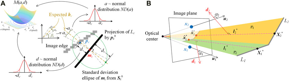
FIGURE 2. Data correspondence (A) and pose optimization (B).

The standard deviation d_c is determined by the distance from m_c to the standard deviational ellipse of m_c along the direction h_c, as illustrated in Figure 2A. The standard deviational ellipse is computed by the covariance propagation of S_k⁰ [see (Liu and Tang, 2023) for details]. As shown in Figure 2A, let β_c ∈ [0,π) be the angle between the horizontal axis of the image plane and h_c, then h_c in Eq. 4 can be rewritten as h_c = ||h_c||₂ [cosβ_c sinβ_c]^T. Supposing β_e is the angle between the horizontal axis of the image plane and the normal line of p_e, then the acute angle a of the normal lines of p_e and m_c can be yielded by a = β_c-β_e. As a result, the variance a_c² of a is computed by a_c² = D (β_c-β_e) = D (β_c), where D means variance. Eventually, a_c can be estimated by the covariance propagation of S_k⁰ in the first order as Eq. 5:

$a_c=\sqrt{\mathrm{D}\left({\beta }_c\right)}=\sqrt{{\nabla }_{{\mathit{p}}^T}{\beta }_c{\mathit{S}}_k^0{\nabla }_{\mathit{p}}{\beta }_c},(5)$

where β_c as well as ${\nabla }_{\mathit{p}}{\beta }_c$ can be computed by

$\begin{array}{l}{\beta }_c=\arctan \left({{\mathit{e}}_2}^T{\mathit{h}}_c/{{\mathit{e}}_1}^T{\mathit{h}}_c\right),\\ {\nabla }_{p^T}{\beta }_c=\left({{\mathit{e}}_2}^T{\nabla }_{{\mathit{p}}^T}{\mathit{h}}_c{{\mathit{e}}_1}^T{\mathit{h}}_c-{{\mathit{e}}_2}^T{\mathit{h}}_c{{\mathit{e}}_1}^T{\nabla }_{{\mathit{p}}^T}{\mathit{h}}_c\right)/{‖{\mathit{h}}_c‖}_2^2,\end{array}(6)$

in which e_i means the 2-dimensional unit vector whose ith component is 1 and the other is 0. In Eq. 6, ${\nabla }_{{\mathit{p}}^T}{\mathit{h}}_c$ can be produced from Eq. 4 as Eq. 7

$\begin{array}{l}{\nabla }_{{\mathit{p}}^T}{\mathit{h}}_c=\left[\begin{array}{cc}{{{\mathit{K}}_{22}}^{-}}^T& {\mathbf{0}}_2\end{array}\right]\left[\begin{array}{cc}{\nabla }_{{\mathit{\Omega }}^T}{\mathit{R}}_k^0{\left[{\mathit{M}}_c\right]}_x{\mathit{N}}_c& {\nabla }_{{\mathit{t}}^T}{\left[{\mathit{t}}_k^0\right]}_x{\mathit{R}}_k^0{\mathit{N}}_c\end{array}\right]\\ =\left[\begin{array}{cc}{{{\mathit{K}}_{22}}^{-}}^T& {\mathbf{0}}_2\end{array}\right]\left[\begin{array}{cc}\left(-{\mathit{R}}_k^0{\left[{\left[{\mathit{M}}_c\right]}_x{\mathit{N}}_c\right]}_x+{\left[{\mathit{t}}_k^0\right]}_x{\mathit{R}}_k^0{\left[{\mathit{N}}_c\right]}_x\right)\mathit{D}\left({\mathit{\Omega }}_k^0\right)& -{\left[{\mathit{R}}_k^0{\mathit{N}}_c\right]}_x\end{array}\right.,\end{array}(7)$

where D (Ω_k⁰) can be calculated by

$\mathit{D}\left({\mathit{\Omega }}_k^0\right)=\frac{{\mathit{\Omega }}_k^0{{\mathit{\Omega }}_k^0}^T}{{‖{\mathit{\Omega }}_k^0‖}^2}-\frac{\sin ‖{\mathit{\Omega }}_k^0‖}{{‖{\mathit{\Omega }}_k^0‖}^3}{{\left[{\mathit{\Omega }}_k^0\right]}_x}^2-\frac{1-\cos ‖{\mathit{\Omega }}_k^0‖}{{‖{\mathit{\Omega }}_k^0‖}^2}{\left[{\mathit{\Omega }}_k^0\right]}_x.(8)$

The derivation of Eq. 8 can be found in (Liu et al., 2020b; Liu and Tang, 2023).

5 Pose determination

This section aimed to determine the 6-DoF pose of the asteroid in real time via the data correspondence provided in Section 4.2 (see the blue box in Figure 1). Compared to the existing edge-based methods (Oumer et al., 2015; Marchand et al., 2019; Liu et al., 2020b; Liu and Tang, 2023), which determine the pose by minimizing the 2D reprojection errors of the 3D features, our method tackles the pose estimation by minimizing the angles between the projection planes of 3D contour segments and the back-projection lines of the corresponding 2D edge points. Such line-to-plane angle is always confined within [0, π/2], which results in the robustness of our method to the size of the target and the relative position of the target to the camera (Huang et al., 2021b). Sufficient experiments verify the outstanding performance of our pose determination method compared to the existing methods (see Section 8 for details).

At instant k, supposing that there are n 3D contour segments {L_ε, ε = 1, 2, … , n}, respectively, corresponding to the 2D edge points {x_ε, ε = 1, 2, … , n}, the back-projection line direction u_ε of each x_ε can be computed by

${\mathit{u}}_{\epsilon }={\mathit{K}}^{-1}{\stackrel{\sim }{\mathit{x}}}_{\epsilon }/{‖{\mathit{K}}^{-1}{\stackrel{\sim }{\mathit{x}}}_{\epsilon }‖}_2.(9)$

The normal vector of the projection plane π_ε of L_ε can be calculated by Eq. 10

${\mathit{d}}_{\epsilon }=\left(\mathit{R}\left(\mathit{\Omega }\right)C_{\epsilon }^1+\mathit{t}\right)\times \left(\mathit{R}\left(\mathit{\Omega }\right)C_{\epsilon }^2+\mathit{t}\right)=\mathit{R}\left(\mathit{\Omega }\right){\mathit{\phi }}_{\epsilon }+{\left[\mathit{t}\right]}_{x}R\left(\mathit{\Omega }\right){\mathit{\varphi }}_{\epsilon },(10)$

where φ_ε = C_ε¹×C_ε² and ϕ_ε = C_ε²−C_ε¹. Let α_ε be the angle between u_ε and d_ε. Then, it is easily known from Figure 2B that minimizing the angle between u_ε and π_ε is equivalent to minimizing |cos α_ε|, which can be simply represented as Eq. 11

$\cos {\alpha }_{\epsilon }=\frac{{\mathit{d}}_{\epsilon }^T}{‖{\mathit{d}}_{\epsilon }^T‖}{\mathit{u}}_{\epsilon }={\mathit{n}}_{\epsilon }^T{\mathit{u}}_{\epsilon }.(11)$

In order to overcome the outlier, we eventually determine the pose p by minimizing the sum of the M-estimator ρ of cosα_ε

$\underset{\mathit{p}}{\min }F\left(\mathit{p}\right)={\displaystyle \sum _{\epsilon =1}^n}\rho \left(\cos {\alpha }_{\epsilon }/\sigma \right)={\displaystyle \sum _{\epsilon =1}^n}\rho \left({{\mathit{n}}_{\epsilon }}^T{\mathit{u}}_{\epsilon }/\sigma \right),(12)$

where σ is set as the median absolute deviation (MAD) of {cosα_ε} with the initial pose p_k⁰ given by the SCKF (see Section 7). In this paper, the Tuckey estimator is used due to its high robustness to outlier (Zhang, 1997). We employ the iterated reweighted least square (IRLS) method to minimize the problem in Eq. 12. Let p^(s) be the pose obtained at iteration step s, and cosα_ε^(s) denotes the cosine of α_ε computed from p^(s). Let v^(s) = [cosα₁^s) cosα₂^s) … cosα_n^(s)]^T. Then, p^(s+1) can be updated by

${\mathit{p}}^{\left(s+1\right)}={\mathit{p}}^{\left(s\right)}-{\left({{\mathit{J}}^{\left(s\right)}}^T{\mathit{W}}^{\left(s\right)}{\mathit{J}}^{\left(s\right)}+\tau {\mathit{I}}_6\right)}^{-1}{{\mathit{J}}^{\left(s\right)}}^T{\mathit{W}}^{\left(s\right)}{\mathit{v}}^{\left(s\right)},(13)$

where τ is a non-negative factor for robustness; W^(s) = diag{…ω(cosα_ε^(s)/σ)…}, in which ω(x) = ρ′(x)/x is the weight function of Tuckey estimator (Zhang, 1997), and J^(s) is the Jacobian matrix of v^(s) and expressed as

${\mathit{J}}^{\left(s\right)}={\left[\begin{array}{ccc}\cdots & {\nabla }_{\mathit{p}}\cos {\alpha }_{\epsilon }^{\left(s\right)}& \cdots \end{array}\right]}^T,(14)$

in which ${\nabla }_{{\mathit{p}}^T}\cos {\alpha }_{\epsilon }\left({\mathit{p}}^{\left(s\right)}\right)$ can be computed by Eq. 15

${\nabla }_{\mathit{p}}\cos {\alpha }_{\epsilon }^{\left(s\right)}={\left.{\mathit{u}}_{\epsilon }^T{\nabla }_{{\mathit{p}}^T}{\mathit{n}}_{\epsilon }\right|}_{\mathit{p}={\mathit{p}}^{\left(s\right)}},(15)$

where ${\nabla }_{{\mathit{p}}^T}{\mathit{n}}_{\epsilon }$ can be computed by

$\begin{array}{l}{\left.{\nabla }_{{\mathit{p}}^T}{\mathit{n}}_{\epsilon }\right|}_{\mathit{p}={\mathit{p}}^{\left(s\right)}}=\left(\frac{1}{‖d_j^{\epsilon }‖}{\mathit{I}}_3-{\mathit{n}}_{\epsilon }{{\mathit{n}}_{\epsilon }}^T\right){\left.{\nabla }_{{\mathit{p}}^T}{\mathit{d}}_{\epsilon }\right|}_{\mathit{p}={\mathit{p}}^{\left(s\right)}}\\ =\left(\frac{1}{‖d_j^{\epsilon }‖}{\mathit{I}}_3-{\mathit{n}}_{\epsilon }{{\mathit{n}}_{\epsilon }}^T\right)\left[\left(-{\mathit{R}}^{\left(s\right)}{\left[{\mathit{\phi }}_{\epsilon }\right]}_x-{\left[{\mathit{t}}^{\left(s\right)}\right]}_x{\mathit{R}}^{\left(s\right)}{\left[{\mathit{\varphi }}_{\epsilon }\right]}_x\right)\mathit{D}\left({\mathit{\Omega }}^{\left(s\right)}\right)-{\left[{\mathit{R}}^{\left(s\right)}{\mathit{\varphi }}_{\epsilon }\right]}_x\right.,\end{array}(16)$

where R^(s) and t^(s) are the rotation matrix and translation vector computed from p^(s), and D (Ω^(s)) has the form of Eq. 8.

6 Covariance estimation of pose

Supposing p^* is the optimal solution of Eq. 12, this section will estimate the covariance matrix V of p^* in the first order, which is used by the SCKF in Section 7 (see the green box in Figure 1). Assuming $\overline{\mathit{p}}$ is the true value of pose p and all edge points have correct correspondence, we can express each of {x_ε} as

${\mathit{x}}_{\epsilon }={\overline{\mathit{x}}}_{\epsilon }+\Delta {\mathit{x}}_{\epsilon },(17)$

where ${\overline{\mathit{x}}}_{\epsilon }$ means the true value of x_ε, and Δx_ε denotes a random perturbation of the true value (Chernov, 2011). All {Δx_ε} are supposed to be independent and follow an identical Gaussian distribution (i.i.d.) with the expectation of zero and the covariance matrix of φ²I₂.

Since p^* is the optimal solution of Eq. 12, p^* must hold the first-order optimality condition of the object function in Eq. 12

${\nabla }_{\mathit{p}}F\left(\mathit{p}\right){|}_{{\mathit{p}}^{*}}={\displaystyle \sum _{\epsilon =1}^n}\omega \left(\cos {\alpha }_{\epsilon }^{*}/\sigma \right){\nabla }_{\mathit{p}}{\mathit{n}}_{\epsilon }^{\ast T}{\mathit{U}}_{\epsilon }{\mathit{n}}_{\epsilon }^{*}={\mathit{0}}_6,(18)$

where U_ε = u_εu_ε^T, n_ε^* = n_ε|_p=p*, cosα_ε^* = u_ε^Tn_ε^*, and ∇_pn_ε^*T can be computed by Eq. 16. We can expand n_ε^*, U_ε^*, and ω(cosα_ε^*) within the vicinity of $\overline{\mathit{p}}$ and ${\overline{\mathit{x}}}_{\epsilon }$ as

$\begin{array}{l}{\mathit{n}}_{\epsilon }^{*}={\overline{\mathit{n}}}_{\epsilon }+{\nabla }_{{\mathit{p}}^T}{\overline{\mathit{n}}}_{\epsilon }\Delta {\mathit{p}}^{*}+O{\left(\Delta {\mathit{p}}^{*}\right)}^2,\\ {\mathit{U}}_{\epsilon }={\overline{\mathit{U}}}_{\epsilon }+{\nabla }_{{{\mathit{x}}_{\epsilon }}^T}{\overline{\mathit{U}}}_{\epsilon }\left(\Delta {\mathit{x}}_{\epsilon }^{*}\otimes {\mathit{I}}_3\right)+O{\left(\Delta {\mathit{x}}_{\epsilon }^{*}\right)}^2,\\ \omega \left(\frac{\cos {\alpha }_{\epsilon }^{*}}{\sigma }\right)=\omega \left(\frac{\cos {\overline{\alpha }}_{\epsilon }}{\sigma }\right)+{\omega }^{\prime }\left(\frac{\cos {\overline{\alpha }}_{\epsilon }}{\sigma }\right)\left({\nabla }_{{\mathit{p}}^T}\left(\frac{\cos {\overline{\alpha }}_{\epsilon }}{\sigma }\right)\Delta {\mathit{p}}^{*}+{\nabla }_{{{\mathit{x}}_{\epsilon }}^T}\left(\frac{\cos {\overline{\alpha }}_{\epsilon }}{\sigma }\right)\Delta {\mathit{x}}_{\epsilon }^{*}\right)+O{\left(\Delta {\mathit{p}}^{*},\Delta {\mathit{x}}_{\epsilon }^{*}\right)}^2,\end{array}(19)$

where the symbol “-” on the top of a variable means the value of the variable computed from ground truth; ${\overline{\mathit{U}}}_{\epsilon }={\overline{\mathit{u}}}_{\epsilon }{{\overline{\mathit{u}}}_{\epsilon }}^T$, $\cos {\overline{\alpha }}_{\epsilon }={\overline{\mathit{n}}}_{\epsilon }^T{\overline{\mathit{u}}}_{\epsilon }$ , $∆{\mathit{p}}^{*}={\mathit{p}}^{*}-\overline{\mathit{p}}$, $\Delta {\mathit{x}}_{\epsilon }={\mathit{x}}_{\epsilon }^{*}-{\overline{\mathit{x}}}_{\epsilon }$; $\otimes$ denotes Kronecker product, and O(x)² denotes the terms of order 2 or higher in x. In Eq. 19, the computation of ${\nabla }_{{\mathit{p}}^T}{\overline{\mathit{n}}}_{\epsilon }$ can be found in Eq. 16, and ${\nabla }_{{{\mathit{x}}_{\epsilon }}^T}{\overline{\mathit{U}}}_{\epsilon }$ can be calculated as

${\nabla }_{{{\mathit{x}}_{\epsilon }}^T}{\overline{\mathit{U}}}_{\epsilon }={\nabla }_{{{\mathit{x}}_{\epsilon }}^T}{\overline{\mathit{u}}}_{\epsilon }\left({\mathit{I}}_2\otimes {{\overline{\mathit{u}}}_{\epsilon }}^T\right)+{\overline{\mathit{u}}}_{\epsilon }{\nabla }_{{{\mathit{x}}_{\epsilon }}^T}{{\overline{\mathit{u}}}_{\epsilon }}^T,(20)$

in which ${\nabla }_{{{\mathit{x}}_{\epsilon }}^T}{\overline{\mathit{u}}}_{\epsilon }$ can be computed from Eq. 9 as Eq. 7

${\nabla }_{{{\mathit{x}}_{\epsilon }}^T}{\overline{\mathit{u}}}_{\epsilon }=\left({\mathit{I}}_3-{\overline{\mathit{U}}}_{\epsilon }\right)\left[\begin{array}{c}{{\mathit{K}}_{22}}^{-1}\\ {{\mathit{0}}_2}^T\end{array}\right]/{‖{\mathit{K}}^{-1}{\stackrel{\sim }{\overline{\mathit{x}}}}_{\epsilon }‖}_2.(21)$

It can be easily noticed that ${\overline{\mathit{n}}}_{\epsilon }^T{\overline{\mathit{u}}}_{\epsilon }=0$. Accordingly, after substituting (19) into (18) and ignoring the higher items, we obtain Eq. 22

$\begin{array}{l}{\mathit{0}}_6={\displaystyle \sum _{\epsilon =1}^n}\omega \left(\frac{\cos {\overline{\alpha }}_{\epsilon }}{\sigma }\right)\left({\nabla }_{\mathit{p}}{{\overline{\mathit{n}}}_{\epsilon }}^T+O\left(\Delta {\mathit{p}}^{*}\right)\right)\left({\overline{\mathit{U}}}_{\epsilon }{\nabla }_{{\mathit{p}}^T}{\overline{\mathit{n}}}_{\epsilon }\Delta {\mathit{p}}^{*}+{\nabla }_{{{\mathit{x}}_{\epsilon }}^T}{\overline{\mathit{U}}}_{\epsilon }\left(\Delta {\mathit{x}}_{\epsilon }^{*}\otimes {\mathit{I}}_3\right){\overline{\mathit{n}}}_{\epsilon }\right)\\ \approx {\displaystyle \sum _{\epsilon =1}^n}\omega \left(\frac{\cos {\overline{\alpha }}_{\epsilon }}{\sigma }\right){\nabla }_{\mathit{p}}{{\overline{\mathit{n}}}_{\epsilon }}^T\left({\overline{\mathit{U}}}_{\epsilon }{\nabla }_{{\mathit{p}}^T}{\overline{\mathit{n}}}_{\epsilon }\Delta {\mathit{p}}^{*}+{\nabla }_{{{\mathit{x}}_{\epsilon }}^T}{\overline{\mathit{U}}}_{\epsilon }\left(\Delta {\mathit{x}}_{\epsilon }^{*}\otimes {\mathit{I}}_3\right){\overline{\mathit{n}}}_{\epsilon }\right),\end{array}(22)$

as a result of which, Δp^* can be obtained by Eq. 23

$\Delta {\mathit{p}}^{*}=-{\mathit{Q}}^{-1}{\displaystyle \sum _{\epsilon =1}^n}\omega \left(\frac{\cos {\overline{\alpha }}_{\epsilon }}{\sigma }\right){\nabla }_{\mathit{p}}{\overline{\mathit{n}}}_{\epsilon }^T{\nabla }_{{{\mathit{x}}_{\epsilon }}^T}{\overline{\mathit{U}}}_{\epsilon }\left(\Delta {\mathit{x}}_{\epsilon }\otimes {\mathit{I}}_3\right){\overline{\mathit{n}}}_{\epsilon },(23)$

where Q can be calculated by Eq. 24

$\mathit{Q}={\displaystyle \sum _{\epsilon =1}^n}\omega \left(\frac{\cos {\overline{\alpha }}_{\epsilon }}{\sigma }\right){\nabla }_{\mathit{p}}{\overline{\mathit{n}}}_{\epsilon }^T{\overline{\mathit{U}}}_{\epsilon }{\nabla }_{{\mathit{p}}^T}{\overline{\mathit{n}}}_{\epsilon }.(24)$

Since {Δx_ε} are i. i.d., then the covariance matrix V of $\Delta {\mathit{p}}^{*}$ is thereby estimated in the first order as Eq. 25

$\begin{array}{l}\mathit{V}=E\left(\Delta {\mathit{p}}^{*}\Delta {\mathit{p}}^{*T}\right)\\ ={\mathit{Q}}^{-1}{\displaystyle \sum _{\epsilon =1}^n}{\displaystyle \sum _{\varsigma =1}^n}\left(\omega \left(\frac{\cos {\overline{\alpha }}_{\epsilon }}{\sigma }\right)\omega \left(\frac{\cos {\overline{\alpha }}_{\varsigma }}{\sigma }\right){\nabla }_{\mathit{p}}{\overline{\mathit{n}}}_{\epsilon }^T{\nabla }_{{{\mathit{x}}_{\epsilon }}^T}{\overline{\mathit{U}}}_{\epsilon }E\left\{\Delta {\mathit{x}}_{\epsilon }\Delta {\mathit{x}}_{\varsigma }^T\otimes {\overline{\mathit{n}}}_{\epsilon }{\overline{\mathit{n}}}_{\varsigma }^T\right\}{\nabla }_{{\mathit{x}}_{\varsigma }}{\overline{\mathit{U}}}_{\varsigma }^T{\nabla }_{{\mathit{p}}^T}{\overline{\mathit{n}}}_{\varsigma }\right){\mathit{Q}}^{-1}\\ ={\phi }^2{\mathit{Q}}^{-1}{\displaystyle \sum _{\epsilon =1}^n}\omega {\left(\frac{\cos {\overline{\alpha }}_{\epsilon }}{\sigma }\right)}^2{\nabla }_{\mathit{p}}{\overline{\mathit{n}}}_{\epsilon }^T{\nabla }_{{{\mathit{x}}_{\epsilon }}^T}{\overline{\mathit{U}}}_{\epsilon }\left({\mathit{I}}_2\otimes {\overline{\mathit{n}}}_{\epsilon }{\overline{\mathit{n}}}_{\epsilon }^T\right){\nabla }_{{\mathit{x}}_{\epsilon }}{\overline{\mathit{U}}}_{\epsilon }^T{\nabla }_{{\mathit{p}}^T}{\overline{\mathit{n}}}_{\epsilon }{\mathit{Q}}^{-1}\\ ={\phi }^2{\mathit{Q}}^{-1}\left({\displaystyle \sum _{\epsilon =1}^n}\omega {\left(\frac{\cos {\overline{\alpha }}_{\epsilon }}{\sigma }\right)}^2{\nabla }_{\mathit{p}}{\overline{\mathit{n}}}_{\epsilon }\left({\nabla }_{{\mathit{x}}_{\epsilon }^1}{\overline{\mathit{U}}}_{\epsilon }{\overline{\mathit{n}}}_{\epsilon }{\overline{\mathit{n}}}_{\epsilon }^T{\nabla }_{{\mathit{x}}_{\epsilon }^1}{\overline{\mathit{U}}}_{\epsilon }^T+{\nabla }_{{\mathit{x}}_{\epsilon }^2}{\overline{\mathit{U}}}_{\epsilon }{\overline{\mathit{n}}}_{\epsilon }{\overline{\mathit{n}}}_{\epsilon }^T{\nabla }_{{\mathit{x}}_{\epsilon }^2}{\overline{\mathit{U}}}_{\epsilon }^T\right){\nabla }_{{\mathit{p}}^T}{\overline{\mathit{n}}}_{\epsilon }\right){\mathit{Q}}^{-1},\end{array}(25)$

where x_ε¹ and x_ε² are the two components of x_ε. It can be noticed from Eq. 20 that ${\nabla }_{{\mathit{x}}_{\epsilon }^i}{\overline{\mathit{U}}}_{\epsilon }{\overline{\mathit{n}}}_{\epsilon }={\overline{\mathit{u}}}_{\epsilon }{{\mathit{e}}_i}^T{\mathit{K}}^{-T}/‖{\mathit{K}}^{-1}{\stackrel{\sim }{\overline{\mathit{x}}}}_{\epsilon }‖$, i = 1, 2, in which e_i denotes the 3-dimensional unit vector whose all components are 0 except the ith component. Therefore, (25) can be rewritten into

$\mathit{V}={\phi }^2{\mathit{Q}}^{-1}\left({\displaystyle \sum _{\epsilon \in G}}\omega {\left(\frac{\cos {\overline{\alpha }}_{\epsilon }}{\sigma }\right)}^2{\nabla }_{\mathit{p}}{\overline{\mathit{n}}}_{\epsilon }^T{\mathit{N}}_{\epsilon }{\mathit{N}}_{\epsilon }^T{\nabla }_{{\mathit{p}}^T}{\overline{\mathit{n}}}_{\epsilon }/{‖{\mathit{K}}^{-1}{\stackrel{\sim }{\overline{\mathit{x}}}}_{\epsilon }‖}_2^2\right){\mathit{Q}}^{-1},(26)$

where ${\mathit{N}}_{\epsilon }=\left[{\overline{\mathit{u}}}_{\epsilon }{{\mathit{e}}_1}^T{\mathit{K}}^{-T}{\overline{\mathit{n}}}_{\epsilon }{\overline{\mathit{u}}}_{\epsilon }{{\mathit{e}}_2}^T{\mathit{K}}^{-T}{\overline{\mathit{n}}}_{\epsilon }\right]$. Eq. 26 provides a theoretical closed-form estimation for the covariance matrix of p^* and cannot be directly used in practice since the true values $\overline{\mathit{p}}$ and {${\overline{\mathit{x}}}_{\epsilon }$} are involved, and all 2D contour points are assumed to have correct correspondence. Actually, p^* is a good approximation to $\overline{\mathit{p}}$. In addition, given the pose p^*, let l_ε^* be the projection of the ray of x_ε on the projection plane π_ε of L_ε (see Figure 2B). Then, the intersection point X_ε^* of l_ε^* with L_ε can be computed by Eq. 27

${{\mathit{X}}_{\epsilon }}^{*}={{{\mathit{C}}_{\epsilon }}^1}^{*}-\frac{{\left({\mathit{u}}_{\epsilon }^{*}\times {\mathit{n}}_{\epsilon }^{*}\right)}^T{{{\mathit{C}}_{\epsilon }}^1}^{*}}{{\left({\mathit{u}}_{\epsilon }^{*}\times {\mathit{n}}_{\epsilon }^{*}\right)}^T\left({{{\mathit{C}}_{\epsilon }}^2}^{*}-{{{\mathit{C}}_{\epsilon }}^1}^{*}\right)}\left({{{\mathit{C}}_{\epsilon }}^2}^{*}-{{{\mathit{C}}_{\epsilon }}^1}^{*}\right),(27)$

where C_ε^1* and C_ε^2* are the coordinate vectors of the endpoints of L_ε in CCS under the pose p^*. The projection point ${{\widehat{\mathit{x}}}_{\epsilon }}^{*}$ of ${{\mathit{X}}_{\epsilon }}^{*}$ can be considered a reasonable approximation to ${\overline{\mathit{x}}}_{\epsilon }$. As a result, in practice, the covariance matrix V of p^* can be approximated reasonably by substituting {$\cos {\overline{\alpha }}_{\epsilon }$} in Eq. 26 with {cosα_ε^*} and replacing $\overline{\mathit{p}}$ and {${\overline{\mathit{x}}}_{\epsilon }$} in Eq. 26 with the p^* and {${{\widehat{\mathit{x}}}_{\epsilon }}^{*}$}, respectively. According to normal distribution, the unbiased estimate to φ in Eq. 26 can be obtained by the MAD of all the components of all the {x_ε-${{\widehat{\mathit{x}}}_{\epsilon }}^{*}$}, as shown in Eq. 28

$\phi =1.4826\underset{\epsilon ,j,i}{\text{Median}}\left(\left|{\mathit{x}}_{\epsilon }^i-{{\widehat{\mathit{x}}}_{\epsilon }^i}^{*}\right|\right),(28)$

where the subscript i means the ith component of the specific vector.

7 Square root cubature Kalman Filter

In this section, the SCKF will provide the final estimation for the pose p and, meanwhile, predict the pose and its covariance for subsequent time instants (see the dashed line box in Figure 1). The predicted pose is the maximum posterior probability estimation (MAP) to the true pose of the next instant via the history of the measurements, and thereby good enough to initialize the subsequent tracking. Furthermore, the final pose updated by SCKF is the MAP to the true pose under the condition of the new and past measurements, thus robust to the influence of illuminance variation, self-occlusion, and image noise. The SCKF is based on the uniform velocity dynamic model, which considers the acceleration of the translation and rotation as random with zero expectation and constant standard deviation. For accuracy, we develop the state model of the SCKF with a 2nd-order auto-regression process, which uses the pose vectors p_k = [Ω_k t_k]^T and p_k-1 = [Ω_k-1 t_k-1] ^T to predict the pose vector p_k+1 = [Ω_k+1 t_k+1]^T at time instant k+1. Let s_k = [Ω_k^T t_k^T Ω_k-1^T t_k-1^T] ^T be the state vector of the SCKF at time instant k (we consider p_-1 = p₀). Then, the state model can be formulated by

$\begin{array}{l}{\mathit{\Omega }}_{k+1}={\log }_{\text{SO}\left(3\right)}\left({\mathit{R}}_k{{\mathit{R}}_{k-1}}^{-1}{\mathit{R}}_k\right)+{\mathit{\Gamma }}_k,\\ {\mathit{t}}_{k+1}={\mathit{R}}_k{{\mathit{R}}_{k-1}}^{-1}\left({\mathit{t}}_k-{\mathit{t}}_{k-1}\right)+{\mathit{t}}_k+{\mathit{\Psi }}_k,\\ {\mathit{\Omega }}_k={\mathit{\Omega }}_k+{\mathit{\eta }}_k,\\ {\mathit{t}}_k={\mathit{t}}_k+{\mathit{\kappa }}_k,\end{array}(29)$

where log_SO3(R) represents the Ω solved from R via (3); Γ_k, Ψ_k, η_k, and κ_k represent the prediction error of the rotation vector and translation vector. All of them are considered Gaussian noise vectors with expectation of zero and variances of τ²I₃, υ²I₃, χ²I₃, and ξ²I₃, respectively. The measurement model of the SCKF can be expressed as

${\mathit{z}}_k=\left[\begin{array}{cc}{\mathit{I}}_6& {\mathit{O}}_6\end{array}\right]{\mathit{s}}_k+{\mathit{\epsilon }}_k,(30)$

where ε_k denotes the measurement error with zero expectation and covariance matrix V_k. At the time instant of k, z_k is determined by the pose determination method in Section 5, and V_k can be directly computed by Eq. 26.

The SCKF is based on Bayesian estimation and Cubature transformation (Arasaratnam and Haykin, 2009). The biggest advantage of SCKF is that it does not make a linear approximation to the non-linear state model in Eq. 29. Thus, the SCKF can effectively improve the accuracy of pose estimation. When k > 0, the corrector and predictor will generate the final pose estimate p_k and the pose prediction, respectively, for the next time instant through the procedures in (Arasaratnam and Haykin, 2009). The pose prediction will be used as the initial value for the subsequent tracking.

8 Experiments

In this section, sufficient synthetic and real trials are performed to validate the proposed method quantitatively and qualitatively on a desktop with a 4.2 GHz CPU, 4 cores, and 16 GB RAM. All algorithms are implemented in MATLAB, except for the data correspondence, which is coded by C++ due to its numerous loops. The 3D models of the asteroids used in the trials are all downloaded from the website (Asteroid, 2024).

8.1 Experimental design

In the synthetic trial, the intrinsic matrix of the simulated CCD camera has a focal length of 700 pixels, an aspect ratio of 1, a skew factor of 0, and an image resolution of 640 × 480 pixels. The asteroids of Kleopatra, Golevka, and HW1 are employed to test our method, whose 3D mesh models are demonstrated in Figures 3A–C. The synthetic trial includes a dark space test, distance test, light test, noise test, model precision test, and initial perturbation test. The dark space test comprehensively examines the performance of our method in a dark environment. In this test, for each asteroid, a sequence of 1,201 image frames is synthesized under sunlight with the Sun phase angle of 45° and Sun attitude angle of 135°. The definition of Sun phase angle and Sun attitude angle is demonstrated in Figure 3D (Zhang et al., 2018; Zhang et al., 2013; Zhang et al., 2015). Kleopatra, Golevka, and HW1 tumble in deep space relative to the CCS with an angular velocity of 0.3° per frame and move away from the camera with the linear velocity of 201.1200 m, 1.3916 m, and 10.0495 m per frame, respectively. The distance test will investigate the robustness of the proposed tracking method to the imaging distance of the asteroid (the distance between the camera and the asteroid). The imaging distance of Kleopatra gradually increases from 380 m to 620 m, the imaging distance of Golevka grows from 1.7 m to 2.8 m, and the imaging distance of HW1 varies from 18 m to 30 m. At each distance level, a sequence of 1,201 image frames is simulated with the angular velocity and the lighting condition used for the dark space test but without linear velocity. Due to the different sizes of the asteroids, the performance is measured with the ratio of the imaging distance of an asteroid to its average radius. The distance-to-radius ratio varies from 6 to 12 with an interval of 1. The light test examines the robustness of the lighting condition. The Sun phase angle gradually changes from 0° to 90° with an interval of 10°. At each phase angle, four image sequences are synthesized with the attitude angles of 0°, 60°, 120°, and 180°, respectively, and the distance-to-radius ratio of 8. The noise test evaluates the robustness of the proposed method to image noise. The zero-mean Gaussian noise is added to the intensities of the image sequence of the distance-to-radius ratio of 8 in the distance test, with the noise level (standard deviation) gradually growing from 2 to 12 with an interval of 2. The intensity value belongs to [0, 255]. The model precision test investigates the influence of the mesh model precision on the proposed tracking method. We gradually reduce the number of the original 3D mesh model facets to 90%, 80%, …, 40%. With each simplified 3D mesh model, we assess the performance of our tracking method with the image sequences of the distance-to-radius ratio of 8 in the distance test. The initial perturbation test assesses the impact of the error of the initial pose on the tracking method with the image sequence of the distance-to-radius ratio of 8 in the distance test. We first perturb the rotation matrix of the initial pose at the beginning of tracking with the rotation error whose MAE gradually increases from 0° to 25° with an interval of 5° and then perturb the translation vector by the translation error with RPE gradually increasing from 0% to 5% with an interval of 0.5%. For each error level of rotation error (translation error), the pose tracking will be performed 10 times. At each time, the tracking system is initialized with an initial pose perturbed by the random rotation error (translation error) with the specific error level. For comparison, Wang’s method (Wang et al., 2023), Tjaden’s method (Tjaden and Schomer, 2017), Marchand’s method (Marchand et al., 2019), and Liu’s method (Liu et al., 2020b) are adopted as reference methods. All these reference methods use image edges to track the 6-DoF pose of the target, thus highly relevant to our proposed methods. All tracking methods are initialized by the method in (Liu et al., 2020b) for the sake of fairness.

FIGURE 3

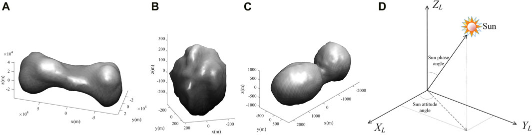
FIGURE 3. 3D mesh models of (A) Kleopatra, (B) Golevka, and (C) HW1; (D) the demonstration of the sun phase and sun attitude angle.

In the real trials, our method will be tested by the 3D-printed physical models of the asteroid Mithra. A calibrated Canon IXUS 65 camera with 30 fps and image resolution of 480 × 640 pixels is adopted to simulate the onboard camera. The Mithra model is placed upon the black backdrop and illuminated by the directional light source so as to simulate the asteroid under a dark space environment. We manually take the video of 1,240 frames for Mithra at different viewpoints. The real trial is tougher than real space missions and synthetic trials due to the random jitter caused by human body shaking.

8.2 Results and analysis

In the synthesis trials, the performance of the tracking method is measured by mean absolute error (MAE), relative position error (RPE), and average CPU runtime. Let R_E and t_E be the estimated rotation matrix and translation of the asteroid, whose true values are R_T and t_T, respectively, and a^x, a^y, and a^z be the three Euler angles recovered from R_ER_T^T with “XYZ” as the order of Euler angle rotations. Then, we define RPE = ||t_E-t_T||₂/||t_T||₂ × 100% and MAE=(|a^x|+|a^y|+|a^z|)/3.

In the dark space test, the performance of all tracking methods is plotted in Figure 4. It can be seen that throughout the tracking process, the pose errors of our method are invariably much lower than Wang’s method, Tjaden’s method, and Marchand’s method, which fail to track the asteroids after the frame of approximately 200. In comparison with Liu’s method, although the performance of our method and Liu’s method are similar, it can be still noticed that the pose errors of our method are lower than that of Liu’s method almost at each frame. During tracking, the largest MAE and RPE of our method for all asteroids are approximately 4.09° and 5.48%, respectively. Table 1 lists the average MAE (AMAE) and average RPE (ARPE) of all methods under the dark space test. It can be found that for each asteroid, the AMAE and ARPE of our method are significantly lower than all the reference methods, several times smaller than that of the second-best method—Liu’s method. Figure 5 shows the percentage of frames with MAE and RPE at less than 1° and 1%, respectively, for all test methods in the dark space test. As seen, for our method, there are at least 85% of frames with MAE less than 1° and RPE less than 1% for all the asteroids, and for each asteroid, the frame percentage achieved by our method is noticeably higher than that of Liu’s method - the second-best method. The CPU runtime of all methods in dark space is listed in Table 2. It is obvious that our tracking method, which is at least 10 times faster than all the reference methods, can estimate the pose from a frame within several milliseconds for all the asteroids. Some example results of our method in the dark space test are demonstrated in Figure 6, where the red lines highlight the projections of the 3D contour segments by the pose estimated by our method, and the number at the upper left corner is the time instant. As revealed, the projections of 3D contour segments are always highly consistent with the asteroids, which qualitatively verifies the accuracy of our proposed method. Due to the fact that our method significantly outperforms all the reference methods in the dark space test, we therefore only test our method in the following tests.

FIGURE 4

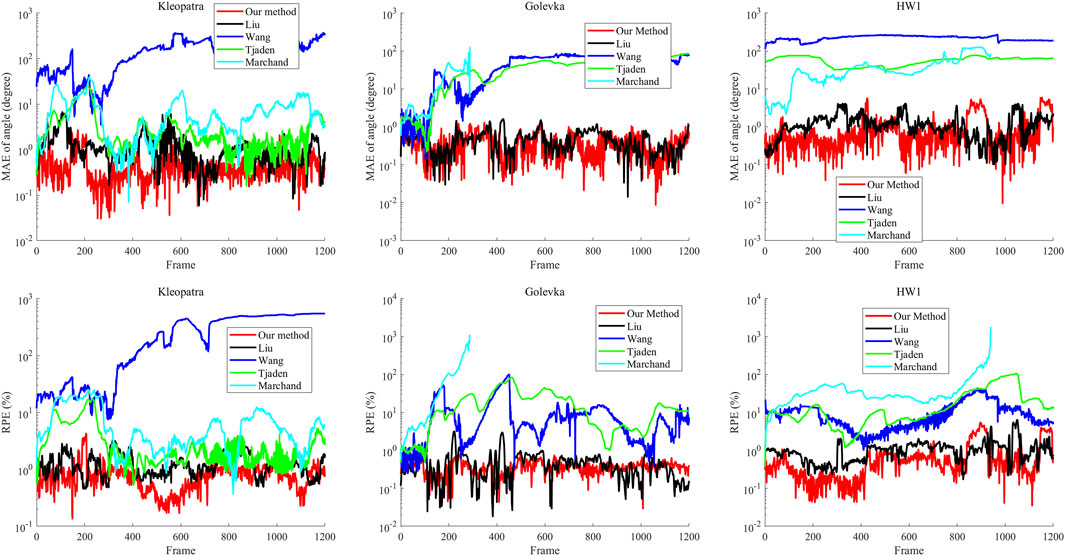
FIGURE 4. MAEs and RPEs of all tracking methods for all asteroids in the dark space test.

TABLE 1

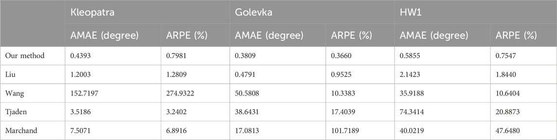
TABLE 1. Average pose error of all methods under the dark space.

FIGURE 5

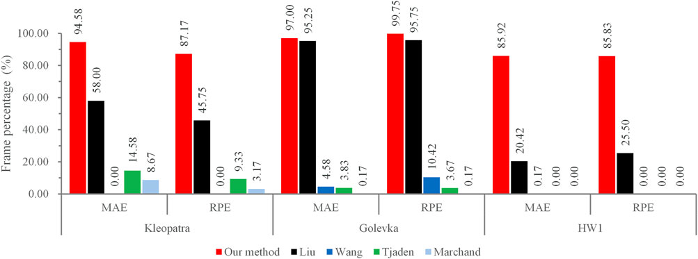
FIGURE 5. The percentage of frames with MAE and RPE less than 1° and 1% under dark space.

TABLE 2

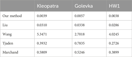
TABLE 2. Average CPU runtime of all tracking methods for all asteroids under the dark space. (s/frame).

FIGURE 6

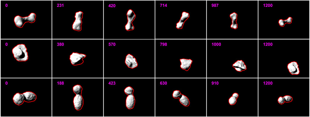
FIGURE 6. Example results of our method in the dark space test for Kleopatra (the top row), Golevka (the middle row), and HW1 (the bottom row).

Figure 7A shows the average pose error of all our methods for all asteroids with the distance-to-radius ratio increasing from 6 to 12 in the distance test. As observed, there is a gentle upward trend on the pose errors of our method with the distance-to-radius ratio rising. This is expected since the asteroid image becomes increasingly small with the distance-to-radius ratio rising. Despite this, the largest AMAE and ARPE of our method for all asteroids are less than approximately 1.5° and 1.8%, respectively. Accordingly, this test validates the robustness of our tracking method to the imaging distance of the asteroids.

FIGURE 7

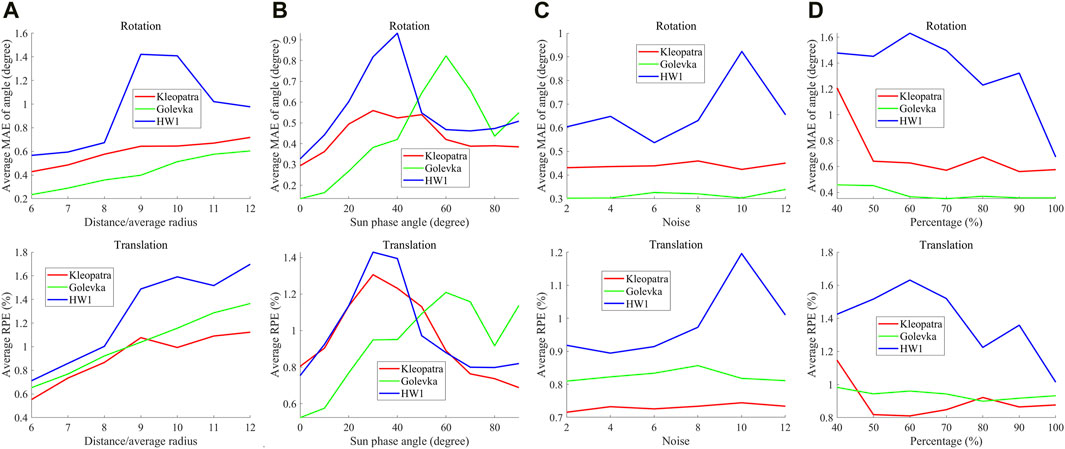
FIGURE 7. Average MAEs and average RPEs of our method in the distance test (A), light test (B), noise test (C), and model precision test (D).

Figure 7B demonstrates the average pose error of our method with the Sun phase angle varying. It can be seen that the tracking errors of Golevka show a noticeable growth with the Sun phase angle. This is perhaps because Golevka looks like a sphere more than the others, which shows that the pose tracking of Golevka is more easily influenced by Sun phase angle. By contrast, the pose errors of HW1 and Kleopatra show some fluctuation as the phase angle increases, which is attributed to the relatively irregular shape of HW1 and Kleopatra. Despite this, our tracking method still achieves acceptable pose accuracy for all the asteroids, with the largest AMAE of approximately 0.9° and the largest APRE of 1.4%, which indicates the satisfactory robustness of our method to illumination.

Figure 7C depicts the average pose errors of our method with the image noise level increasing. As seen, there are almost no increases in the pose errors of Kleopatra and Golevka as the noise level grows. The AMAE and APRE of Kleopatra almost level off at approximately 0.45° and 0.7%, respectively, and the AMAE and APRE of Golevka stay at approximately 0.3° and 0.8%, respectively. By comparison, there exists a slight rise in the pose errors of HW1. This is because the shape of HW1 is more irregular than the others, which makes the pose tracking of HW1 relatively more sensitive to image noise. Nonetheless, the AMAE and APRE of HW1 are still less than approximately 1° and 1.1%, respectively. Therefore, it can be concluded that the proposed tracking method is fairly robust to the noise in the asteroid image.

Figure 7D illustrates the average pose errors of the proposed method as model precision increases. It is obvious that the pose errors of all asteroids show a noticeable drop with the model precision rising. This is expected since the precise model can reduce the mismatching between the extracted 3D contour segments and the 2D edge points. It should be noticed that for all asteroids, the tracking errors are still small enough even though the facets of the mesh models are reduced to 40%, whose corresponding AMAE and APRE are smaller than 1.6° and 1.6%, respectively. In consequence, this test verifies the good robustness of the proposed tracking method to mesh model precision.

Figure 8 shows the AMAE and ARPE of the proposed method with the initial pose error increasing. As seen, the pose errors of all the asteroids show a slight growth when the initial rotation error increases from 0° to 15°, and soar thereafter. Similarly, the pose errors of all the asteroids show a gentle fluctuation as the initial translation error increases from 0 to approximately 3.5%, and surges after that. This is expected since a large initial pose error may lead to more serious 2D-3D mismatching. Despite this, it is noteworthy that the AMAE and ARPE of all the asteroids are smaller than approximately 2° and 2%, respectively, when the rotation error level and the translation error level are less than around 15° and 3.5%, respectively. Accordingly, this trial indicates that the initial pose error with RPE less than 3.5% and MAE less than 15° has little impact on the proposed method.

FIGURE 8

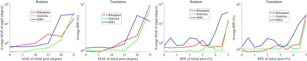
FIGURE 8. Average pose errors of our method in the initial pose error test.

The real trial will validate the proposed method qualitatively in reality because the ground truth of the pose is unknown. Figure 9 displays some example results of pose tracking, where the magenta numbers indicate the time instants and green lines represent the projected 3D contour segments via the estimated pose. The consistency between the projected contour and the target external silhouette validates the efficacy of our tracking method in real scenes. The CPU runtime for Mithra is 0.0058 s/frame, which accords with the CPU runtime reported in Table 2. Consequently, this real trial confirms the prominent accuracy and efficiency of our method in reality. Supplementary Video S1 demonstrates the whole tracking of Mithra.

FIGURE 9

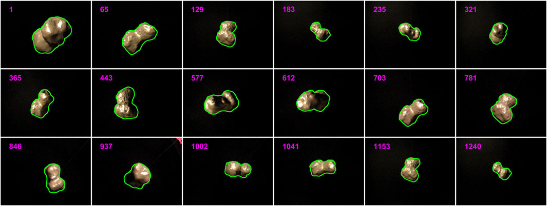
FIGURE 9. Example results of our method for Mithra in the real trial.

9 Conclusion

In this paper, we propose a monocular framework to track the 6-DoF pose of asteroids in real time using the 3D contour of the asteroid. Given the 3D mesh model of the asteroid, at the beginning time instant of the pose tracking, the tracking system is initialized by a pose retrieval method. At each subsequent instant, with the initial pose and its covariance given by the SCKF, the 3D segments constituting the 3D contour of the asteroid are extracted from the 3D mesh model. Then in the input image, the 2D edge points corresponding to the 3D contour segments are retrieved within the range decided by the initial pose and its covariance. The asteroid pose is then determined in real time by minimizing the angles between the back-projection lines of the 2D edge points and the projection planes of the corresponding 3D contour segments with M-estimation. Subsequently, the first-order covariance of the estimated pose is computed, and eventually, by means of this covariance matrix, the 2nd-AR-based SCKF generates the final pose estimate and predicts the initial pose and its covariance for the next instant. Sufficient synthetic and real trials have validated that the proposed method outperforms the existing methods in terms of accuracy and efficiency.

Data availability statement

The original contributions presented in the study are included in the article/Supplementary Material, further inquiries can be directed to the corresponding author.

Author contributions

CL: Methodology, Writing–original draft. HT: Formal Analysis, Software, Writing–original draft. YS: Software, Writing–review and editing. QW: Software, Writing–review and editing. WH: Project administration, Supervision, Writing–review and editing.

Funding

The author(s) declare financial support was received for the research, authorship, and/or publication of this article. This work is supported by the National Key R&D Plan (Grant No. 2020YFC2004400), the Natural Science Foundation of Guangdong Province (Grant No. 2021A1515011678), the National Natural Science Foundation of China (Grant No. 62273324), and the Cooperation on Scientific and Technological Innovation in Hong Kong, Macao, and Taiwan as Part of the National Key R&D Programs (Grant No. 2021YFE0204300).

Conflict of interest

The authors declare that the research was conducted in the absence of any commercial or financial relationships that could be construed as a potential conflict of interest.

Publisher’s note

All claims expressed in this article are solely those of the authors and do not necessarily represent those of their affiliated organizations, or those of the publisher, the editors and the reviewers. Any product that may be evaluated in this article, or claim that may be made by its manufacturer, is not guaranteed or endorsed by the publisher.

Supplementary material

The Supplementary Material for this article can be found online at: https://www.frontiersin.org/articles/10.3389/frspt.2024.1337262/full#supplementary-material

References

Arasaratnam, I., and Haykin, S. (2009). Cubature Kalman filters. IEEE Trans. automatic control 54 (6), 1254–1269. doi:10.1109/tac.2009.2019800

CrossRef Full Text | Google Scholar

Asteroid (2024). The website of 3D asteroid model. https://3d-asteroids.space/.

Google Scholar

Black, K., Shankar, S., Fonseka, D., Deutsch, J., Dhir, A., and Akella, M., real-time flight-ready noncooperative spacecraft pose estimation using monocular imagery, https://arxiv.org/abs/2101.09553 (2021)

Google Scholar

Bray, M., Kohli, P., and Torr, P. (2006). “POSECUT: simultaneous segmentation and 3D pose estimation of humans using dynamic graph-cuts,” in Proc. Of European conf. On comput. Vis. Springer, (Graz, Austria), 642–655.

CrossRef Full Text | Google Scholar

Brox, T., Rosenhahn, B., and Weichert, J. (2005). Three-dimensional shape knowledge for joint image segmentation and pose estimation. Jt. Pattern Recognit. Symp. 3663, 109–116. doi:10.1007/11550518_14

CrossRef Full Text | Google Scholar

Cao, Z., Sheikh, Y., and Banerjee, N. (2016). Real-time scalable 6DOF pose estimation for textureless objects. Stockholm, Sweden: Proceedings of the 2016 IEEE Int. Conf. on Robotics and Automation, 2441–2448.

Google Scholar

Capuano, V., Kim, K., Harvard, A., and Chung, S. J. (2020). Monocular-based pose determination of uncooperative space objects. Acta Astronaut. 166, 493–506. doi:10.1016/j.actaastro.2019.09.027

CrossRef Full Text | Google Scholar

Cassinis, L., Menicucci, A., Gill, E., Ahrns, I., and Sanchez-Gestido, M. (2022). On-ground validation of a CNN-based monocular pose estimation system for uncooperative spacecraft: bridging domain shift in rendezvous scenarios. Acta Astronaut. 196, 123–138. doi:10.1016/j.actaastro.2022.04.002

CrossRef Full Text | Google Scholar

Chen, B., Cao, J., Parra, A., and Chin, T. (2019). Satellite pose estimation with deep landmark regression and nonlinear pose refinement. Seoul, South Korea: Proceedings of the IEEE/CVF Int. Conf. on Comput. Vis. Workshop.

CrossRef Full Text | Google Scholar

Chernov, N. (2011). Fitting geometric curves to observed data. https://citeseerx.ist.psu.edu/document?repid=rep1&type=pdf&doi=c501b06f22abe1a20f316848cd69d8b642426be.

Google Scholar

Christian, J. (2015). Optical navigation using planet’s centroid and apparent diameter in image. J. Guid. control, Dyn. 38 (2), 192–204. doi:10.2514/1.g000872

CrossRef Full Text | Google Scholar

Comellini, A., Zenou, E., Espinosa, C., and Dubanchet, V. (2020). Vision-based navigation for autonomous space rendezvous with non-cooperative targets, Proceedings of the 11th international conference on information intelligence systems and applications, Greece, Piraeus.

CrossRef Full Text | Google Scholar

Conway, D., Macomber, B., Cavalieri, , and Junkins, J. (2014). Vision-based relative navigation filter for asteroid rendezvous, Proceedings of the AAS Guidance, Navigation, and Control Conference, Breckenridge, CO, USA.

Google Scholar

Crivellaro, A., Rad, M., Verdie, Y., Yi, K., Fua, P., and Lepetit, V. (2017). Robust 3D object tracking from monocular images using stable parts. IEEE Trans. pattern analysis Mach. Intell. 40 (6), 1465–1479. doi:10.1109/tpami.2017.2708711

PubMed Abstract | CrossRef Full Text | Google Scholar

Dambreville, S., Sandhu, R., Yezzi, A., and Tannenbaum, A. (2008). “Robust 3D pose estimation and efficient 2D region-based segmentation from a 3D shape prior,” in Proc. Of European conf. On comput. Vis. (Marseille, France), Springer, 169–182.

CrossRef Full Text | Google Scholar

Forshaw, J., Aglietti, G., Navarathinam, N., Kadhem, H., Salmon, T., Pisseloup, A., et al. (2016). RemoveDEBRIS: an in-orbit active debris removal demonstration mission. Acta Astronaut. 127, 448–463. doi:10.1016/j.actaastro.2016.06.018

CrossRef Full Text | Google Scholar

Golish, D., d’Aubigny, C., Rizk, B., DellaGiustina, D., Smith, P., Becker, K., et al. (2020). Ground and in-flight calibration of the OSIRIS-REx camera suite. Space Sci. Rev. 216, 1–31. doi:10.1007/s11214-019-0626-6

PubMed Abstract | CrossRef Full Text | Google Scholar

He, Z., Jiang, Z., Zhao, X., Zhang, S., and Wu, C. (2020). Sparse template-based 6-D pose estimation of metal parts using a monocular camera. IEEE Trans. Industrial Electron. 67 (1), 390–401. doi:10.1109/tie.2019.2897539

CrossRef Full Text | Google Scholar

Hearn, D., and Baker, M. (2005). Computer graphics with OpenGL. Beijing, China: Publishing House of Electronics Industry.

Google Scholar

Hexner, J., and Hagege, R. (2016). 2D-3D pose estimation of heterogeneous objects using a region based approach. Int. J. Comput. Vis. 118, 95–112. doi:10.1007/s11263-015-0873-2

CrossRef Full Text | Google Scholar

Hu, Y., Speiere, S., Jakob, W., Fua, P., and Salzmann, M. (2021). Wide-depth-range 6D object pose estimation in space. Proc. IEEE/CVF Conf. Comput. Vis. Pattern Recognit., 15870–15879. doi:10.1109/CVPR46437.2021.01561

CrossRef Full Text | Google Scholar

Huang, H., Zhao, G., Gu, D., and Bo, Y. (2021a). Non-model-based monocular pose estimation network for uncooperative spacecraft using convolutional neural network. IEEE Sens. J. 21 (21), 24579–24590. doi:10.1109/jsen.2021.3115844

CrossRef Full Text | Google Scholar

Huang, H., Zhong, F., Sun, Y., and Qin, X. (2020). An occlusion-aware edge-based method for monocular 3d object tracking using edge confidence. Comput. Graph. Forum 39 (7), 399–409. doi:10.1111/cgf.14154

CrossRef Full Text | Google Scholar

Huang, Y., Zhang, Z., Cui, H., and Zhang, L. (2021b). A low-dimensional binary-based descriptor for unknown satellite relative pose estimation. Acta Astronaut. 181, 427–438. doi:10.1016/j.actaastro.2021.01.050

CrossRef Full Text | Google Scholar

Huo, Y., Li, Z., and Zhang, F. (2020). Fast and accurate spacecraft pose estimation from single shot space imagery using box reliability and keypoints existence judgments. IEEE Access 8, 216283–216297. doi:10.1109/access.2020.3041415

CrossRef Full Text | Google Scholar

Kanani, K., Petit, A., Marchand, E., Chabot, T., and Gerber, B. (2012). “Vision-based navigation for debris removal missions,” in Proc. Of 63rd int. Astronautical congr. (Naples, Italy), HAL, 1–8.

Google Scholar

Kelsey, J., Byrne, J., Cosgrove, M., Seereeram, S., and Mehra, R. (2006). “Vision-based relative pose estimation for autonomous rendezvous and docking,” in Proceedings of the 2006 IEEE Aerospace Conference (Big Sky, MT, USA), 1–20.

Google Scholar

Kobayashi, N., Oyamada, Y., Mochizuki, Y., and Ishikawa, H. (2015). Three-DoF pose estimation of asteroids by appearance-based linear regression with divided parameter space. Tokyo, Japan: Proceedings of the 14th IAPR International Conference on Machine Vision Applications, 551–554.

CrossRef Full Text | Google Scholar

Lentaris, G., Stratakos, I., Stamoulias, I., Soudris, D., Lourakis, M., and Zabulis, X. (2020). High-performance vision-based navigation on SoC FPGA for spacecraft proximity operations. IEEE Trans. Circuits Syst. Video Technol. 30 (4), 1188–1202. doi:10.1109/tcsvt.2019.2900802

CrossRef Full Text | Google Scholar

Leroy, B., Medioni, G., Johnson, E., and Matthies, L. (2001). Crater detection for autonomous landing on asteroids. Image Vis. Comput. 19, 787–792. doi:10.1016/s0262-8856(00)00111-6

CrossRef Full Text | Google Scholar

Li, M., and Xu, B. (2018). Autonomous orbit and attitude determination for earth satellites using images of regular-shaped ground objects. Aerosp. Sci. Technol. 80, 192–202. doi:10.1016/j.ast.2018.07.019

CrossRef Full Text | Google Scholar

Liu, C., Guo, W., Hu, W., Chen, R., and Liu, J. (2023). Real-time crater-based monocular 3-D pose tracking for planetary landing and navigation. IEEE Trans. Aerosp. Electron. Syst. 59 (1), 311–335. doi:10.1109/taes.2022.3184660

CrossRef Full Text | Google Scholar

Liu, C., Guo, W., Hu, W., Chena, R., and Liu, J. (2020b). Real-time model-based monocular pose tracking for an asteroid by contour fitting. IEEE Trans. Aerosp. Electron. Syst. 57 (3), 1538–1561. doi:10.1109/taes.2020.3044116

CrossRef Full Text | Google Scholar

Liu, C., GuoHu, W. W., Chena, R., and Liu, J. (2020a). Real-time vision-based pose tracking of spacecraft in close range using geometric curve fitting. IEEE Trans. Aerosp. Electron. Syst. 56 (6), 4567–4593. doi:10.1109/taes.2020.2996074

CrossRef Full Text | Google Scholar

Liu, C., and Hu, W. (2013). Effective method for ellipse extraction and integration for spacecraft images. Opt. Eng. 52 (5), 057002. doi:10.1117/1.oe.52.5.057002

CrossRef Full Text | Google Scholar

Liu, C., and Hu, W. (2014). Relative pose estimation for cylinder-shaped spacecrafts using single image. IEEE Trans. Aerosp. Electron. Syst. 50 (4), 3036–3056. doi:10.1109/taes.2014.120757

CrossRef Full Text | Google Scholar

Liu, C., and Tang, H. (2023). Model-based visual 3D pose tracking of non-cooperative spacecraft in Close Range. Baku, Azerbaijan: Proceedings of the 74th International Astronautical Congress.

Google Scholar

Long, C., and Hu, Q. (2022). Monocular-vision-based relative pose estimation of noncooperative spacecraft using multicircular features. IEEE/ASME Trans. Mechatronics 27 (6), 5403–5414. doi:10.1109/tmech.2022.3181681

CrossRef Full Text | Google Scholar

Lourakis, M., and Zabulis, X. (2017). “Model-based visual tracking of orbiting satellites using edges,” in Proceedings of the 2017 IEEE/RSJ International Conference on Intelligent Robots and Systems (IROS) (Vancouver, Canada), 3791–3796.

CrossRef Full Text | Google Scholar

Marchand, E., Chaumette, F., Chabot, T., Kanani, K., and Polinni, A. (2019). RemoveDebris vision-based navigation preliminary results. Washington, DC, USA. HAL.

Google Scholar

Meng, C., Li, Z., Sun, H., Yuan, D., Bai, X., and Zhou, F. (2018). Satellite pose estimation via single perspective circle and line. IEEE Trans. Aerop. Electron. Syst. 54 (6), 3084–3095. doi:10.1109/taes.2018.2843578

CrossRef Full Text | Google Scholar

Opromolla, R., Fasano, G., Rufino, G., and Grassi, M. (2017). A review of cooperative and uncooperative spacecraft pose determination techniques for close-proximity operations. Prog. Aerosp. Sci. 93, 53–72. doi:10.1016/j.paerosci.2017.07.001

CrossRef Full Text | Google Scholar

Oumer, N., Panin, G., Mülbauer, Q., and Tseneklidou, A. (2015). Vision-based localization for on-orbit servicing of a partially cooperative satellite. Acta Astronaut. 117, 19–37. doi:10.1016/j.actaastro.2015.07.025

CrossRef Full Text | Google Scholar

Park, T., and Amico, S. (2023). Robust multi-task learning and online refinement for spacecraft pose estimation across domain gap. Adv. Space Res., doi:10.1016/j.asr.2023.03.036

CrossRef Full Text | Google Scholar

Peng, J., Xu, W., Yan, L., Pan, E., Liang, B., and Wu, A. G. (2020). A pose measurement method of a space non-cooperative target based on maximum outer contour recognition. IEEE Trans. Aerop. Electron. Syst. 50 (1), 512–526. doi:10.1109/taes.2019.2914536

CrossRef Full Text | Google Scholar

Petit, A., Marchand, E., and Kanani, K. (2012a). “Tracking complex targets for space rendezvous and debris removal applications,” in Proceedings of the 2012 IEEE/RSJ International Conference on Intelligent Robots and Systems (Vilamoura, Portugal), 4483–4488.

CrossRef Full Text | Google Scholar

Petit, A., Marchand, E., and Kanani, K. (2012b). “Vision-based detection and tracking for space navigation,” in Proc. Of int. Symp. On artificial intell., robot. And autom. In space Washington, DC, USA. HAL.

Google Scholar

Phisannupawong, T., Kamsing, P., Torteeka, P., Channumsin, S., Sawangwit, U., Hematulin, W., et al. (2020). Vision-based spacecraft pose estimation via a deep convolutional neural network for noncooperative docking operations. Aerospace 7 (9), 126. doi:10.3390/aerospace7090126

CrossRef Full Text | Google Scholar

Prisacariu, V., and Reid, I. (2012). PWP3D: real-time segmentation and tracking of 3D objects. Int. J. Comput. Vis. 98 (3), 335–354. doi:10.1007/s11263-011-0514-3

CrossRef Full Text | Google Scholar

Prisacariu, V., Segal, A., and Reid, I. (2012). Simultaneous monocular 2D segmentation, 3D pose recovery and 3D reconstruction. Asian Conf. Comput. Vis., 593–606. doi:10.1007/978-3-642-37331-2_45

CrossRef Full Text | Google Scholar

Proença, P., and Gao, Y. (2020). “Deep learning for spacecraft pose estimation from photorealistic rendering,” in Proceedings of the IEEE international conference on robotics and automation (IEEE), Paris, France, 6007–6013.

Google Scholar

Pugliatti, M., and Topputo, F. (2022). Navigation about irregular bodies through segmentation maps. Adv. Astronautical Sci. 176, 1169–1187.

Google Scholar

Rathinam, A., Gaudilliere, V., Pauly, L., and Aouada, D. (2022). Pose estimation of a known texturless space target using convolutional neural network. Paris, France: International Astronautical Congress, 18–22.

Google Scholar

Raytchev, B., Terakado, K., Tamaki, T., and Kaneda, K. (2011). Pose estimation by local procrustes regression. Brussels, Belgium: Proceedings of the 18th IEEE International Conference on Image Processing, 3585–2588.

CrossRef Full Text | Google Scholar

Rondao, D., Aouf, N., Richardson, M., and Dubanchet, V. (2021). Robust on-manifold optimization for uncooperative space relative navigation with a single camera. J. Guid. Control, Dyn. 44 (6), 1157–1182. doi:10.2514/1.g004794

CrossRef Full Text | Google Scholar

Rowell, N., Dunstan, M., Parkes, S., Gil-Fernández, J., Huertas, I., and Salehi, S. (2015). Autonomous visual recognition of known surface landmarks for optical navigation around asteroids. Aeronautical J. 119 (1220), 1193–1222. doi:10.1017/s0001924000011210

CrossRef Full Text | Google Scholar

Sattler, T., Zhou, Q., Pollefeys, M., and Leal-Taix´e, L. (2019). Understanding the limitations of CNN-based absolute camera pose regression. Long Beach, CA, USA: Proceedings of the 2019 IEEE/CVF Conf. on Comput. Vis. and Pattern Recognit.

CrossRef Full Text | Google Scholar

Sharma, S., Beierle, C., and D'Amico, S. (2018). “Pose estimation for non-cooperative spacecraft rendezvous using convolutional neural networks,” in Proceedings of the 2018 IEEE Aerospace Conference (Big Sky, MT, USA), 1–23.

CrossRef Full Text | Google Scholar

Sharma, S., and Amico, S. (2020). Neural network-based pose estimation for noncooperative spacecraft rendezvous. IEEE Trans. Aerop. Electron. Syst. 56 (6), 4638–4658. doi:10.1109/taes.2020.2999148

CrossRef Full Text | Google Scholar

Sonawani, S., Alimo, R., Detry, R., Jeong, D., Hess, A., and Amor, H. (2020). Assistive relative pose estimation for on-orbit assembly using convolutional neural networks. https://arxiv.org/abs/2001.10673.

Google Scholar

Stacey, N., and Amico, S. (2018). Autonomous swarming for simultaneous navigation and asteroid characterization. Snowbird, UT, USA: Proceedings of the 2018 AAS/AIAA Astrodynamics Specialist Conference.

Google Scholar

Stoiber, M., Pfanne, M., Strobl, K., Triebel, R., and Albu-Schäffer, A. (2022). SRT3D: a sparse region-based 3D object tracking approach for the real world. Int. J. Comput. Vis. 130 (4), 1008–1030. doi:10.1007/s11263-022-01579-8

CrossRef Full Text | Google Scholar

Sugita, S., Honda, R., Morota, T., Kameda, S., Sawada, H., Tatsumi, E., et al. (2019). The geomorphology, color, and thermal properties of Ryugu: implications for parent-body processes. Science 364 (6437), 252. doi:10.1126/science.aaw0422

PubMed Abstract | CrossRef Full Text | Google Scholar

Suzuki, S., and Abe, K. (1985). Topological structural analysis of digitized binary images by border following. Comput. Vis. Graph. Image Process. 30 (1), 32–46. doi:10.1016/0734-189x(85)90016-7

CrossRef Full Text | Google Scholar

Tjaden, H., and Schomer, E. (2017). Real-time monocular pose estimation of 3D objects using temporally consistent local color histograms. Proc. IEEE Int. Conf. Comput. Vis., 124–132. doi:10.1109/ICCV.2017.23

CrossRef Full Text | Google Scholar

Wang, Q., Zhou, J., Li, Z., Sun, X., and Yu, Q. (2023). Robust monocular object pose tracking for large pose shift using 2D tracking. Vis. Intell. 1 (1), 22. doi:10.1007/s44267-023-00023-w

CrossRef Full Text | Google Scholar

Watanabe, S., Tsuda, Y., Yoshikawa, M., Tanaka, S., Saiki, T., and Nakazawa, S. (2017). Hayabusa2 mission overview. Space Sci. Rev. 208, 3–16. doi:10.1007/s11214-017-0377-1

CrossRef Full Text | Google Scholar

Zhang, H., Jiang, Z., and Elgammal, A. (2013). Vision-based pose estimation for cooperative space objects. Acta Astronaut. 91 (10), 115–122. doi:10.1016/j.actaastro.2013.05.017

CrossRef Full Text | Google Scholar

Zhang, H., Jiang, Z., and Elgammal, A. (2015). Satellite recognition and pose estimation using homeomorphic manifold analysis. IEEE Trans. Aerosp. Electron. Syst. 51 (1), 785–792. doi:10.1109/taes.2014.130744

CrossRef Full Text | Google Scholar

Zhang, X., Jiang, Z., Zhang, H., and Wei, Q. (2018). Vision-based pose estimation for textureless space objects by contour points matching. IEEE Trans. Aerosp. Electron. Syst. 54 (5), 2342–2355. doi:10.1109/taes.2018.2815879

CrossRef Full Text | Google Scholar

Zhang, Z. (1997). Parameter estimation techniques: a tutorial with application to conic fitting. Image Vis. Comput. 15 (1), 59–76. doi:10.1016/s0262-8856(96)01112-2

CrossRef Full Text | Google Scholar

Zhong, L., Zhao, X., Zhang, Y., Zhang, S., and Zhang, L. (2020). Occlusion-Aware region-based 3D pose tracking of objects with temporally consistent polar-based local partitioning. IEEE Trans. Image Process. 29, 5065–5078. doi:10.1109/tip.2020.2973512

PubMed Abstract | CrossRef Full Text | Google Scholar

Zhou, D., Sun, G., and Hong, X. (2021). 3D visual tracking framework with deep learning for asteroid exploration. https://arxiv.org/abs/2111.10737.

Google Scholar