Evaluation and visualization of a rectangle’s gravity on its surface, and on spheres inside, outside, or intersecting it

For convenient comparison and clear physical meaning, the gravity on the surface of a homogeneous cube and on spheres inside, outside, and intersecting about it is calculated by polyhedral or harmonic expansion methods. In addition, the gravity coefficients of a rectangle’s spherical harmonics are both derived analytically and evaluated numerically, where only five terms are nontrivial up to the order of 4, which is somewhat unexpected when we first obtained them. There are some similarities of these coefficients to an ellipsoid for the terms $C_{20},C_{22},C_{42}$, but they are much different for the terms $C_{40},C_{44}$. Thence, a few special gravity characteristics are here revealed or visualized. For example, it is shown as expected that the maximum gravity appears at the sphere intersecting the cube, but maximum surface gravity at the center of the mid-plane of a rectangle’s surface is different from the gravity on an ellipsoid at the end of its short axis. Based on these results, an orbit around a cube is integrated by a polyhedral method, and its secular motion analysis by averaging theory is investigated where the numerical and analytic results fit very well. Finally, a few special trajectories on a surface plane of a cube are simulated; the physical meaning is quite clear, and some insights are shown, such as why a natural celestial body in the shape of a rectangle with sharp corners is rarely found due to its surface gravity distribution. All gravity calculations are visualized on 3D figures both for cubes or rectangles. Additionally, examples of an asteroid and an ellipsoid are shown so that the techniques discussed here can be adopted to directly analyzing the gravity of other shapes.

1 Introduction

A cube’s or a rectangle’s gravity is of interest to researchers in areas including the theoretical analysis in the history of gravity research (MacMillan, 1958; Waldvogel, 1976; Nagy, 1966; Banerjee and Buddhadeb, 1977; Michalodimitrakis and Bozis, 1985), mission design around irregular bodies (Werner, 1994; Hu and Scheeres, 2002; Chappel and Abbott, 2012), and the application of satellite gravity to mission design or gradiometry (Venditti and Prado, 2019; Liu et al., 2011; Parikh and Tewari, 2021). Much of this research addresses the potential and gravity of rectangles, but little of it discusses the gravity on surface of a rectangle, and very little calculates the gravity inside a rectangle.

Modeling the gravity near a celestial body is an important issue for spacecraft landing, taking off, and flying around it (Scheeres et al., 1996; Hu and Scheeres, 2004; Hu and Scheeres, 2014; Herrera et al., 2013; Hu, 2015), especially for irregular bodies (Mysen et al., 2006; Fukushima, 2017; Pinson and Lu, 2019; Nikolaeva et al., 2019; Valvano et al., 2022). The key issue in all this research is modeling the gravity around irregular asteroids. While many methods have been studied, the most efficient approaches are harmonic expansion and polyhedral models, which are respectively fast and precise in computation.

Just like an ellipsoid (Guibout and Scheeres, 2003; Dobrovolskis, 2019), a rectangle is also a basic element in the structure of gravity research. A really complicated shape can be composed of these elements, such as ellipsoids and rectangles. A cube could be used to simulate some special asteroids whose shape is similar to a cube, or a part of irregularly shaped asteroids. For example, the shape of asteroid 4,769 Casterlia (Hudson and Ostro, 1994) is similar to a rectangle, or, more accurately, it can be regarded as two connected cubes with smooth corners. Extended discussion about this asteroid is given at the end of this paper. The most important characteristic of a cube’s gravity is that its physical meaning and pattern are clear, such as the gravity distribution on its surface, which is helpful for understanding the nature of near-central body gravity, including for asteroids. Another example is the recently discovered mystery object with many uncertainties, 1I/2017U1(Oumuamua) (Bannister et al., 2019), which recently passed through our solar system. It is remarkable not only because of its unique orbital eccentricity of about 1.2 and its probably being an interstellar asteroid, but also due to its very elongated shape with sharp edges and near planar surface. Its extreme axis ratio is at least 6:1, and even probably up to 10:1 ($400\times 40\times$40 m). A simple rectangular model with some analytical solutions for its preliminary gravity analysis is definitely meaningful and practicable here. It is well known that we cannot derive simple analytical conclusions for complicated models such as high dimensional polyhedral models with thousands of vertices (Hudson and Ostro, 1994).

Many have studied the gravity fields of asteroids as an example of irregularly shaped bodies. Werner and Scheeres (1997) proposed the application of polyhedral methods to evaluate the exterior gravitational field on irregularly shaped asteroids; they calculated and compared acceleration magnitudes mainly on different special planes such as $x=0,y=0$ or $z=0$. Takahashi et al. (2013) calculated both exterior and interior spherical harmonic coefficients to model the near surface gravity of an asteroid. More recently, Sebera et al. (2016) evaluated the gravity field of an asteroid by spheroidal models.

This study discusses the parallel gravity of an ellipsoid or an asteroid to rectangles with the same objectives to reveal some aspects of the basic nature in gravities of different shapes by different methods, with some special analytical conclusions. The remainder of this article is organized as follows. Section 2 briefly introduces the definitions of harmonic expansion and the polyhedral method, including the coordinate transformation of derivatives. In Section 3, the 3D and 2D gravity distributions of cubes are plotted, then the harmonic expansion coefficients up to the sixth degree and order are calculated. For comparative convenience, a rectangle’s surface gravity and harmonic coefficients are assessed, including their analytical formulation. Many examples of gravity accelerations both on surfaces on and spheres around a cube are then calculated, including motion examples and analysis, and many comparisons given. Finally, Section 5 provides conclusions, explanations, and also some extensions to an asteroid and an ellipsoid.

2 Gravity calculation method

2.1 Spherical harmonic expansion

The spherical harmonic gravity field is widely adopted with coefficients associated with Legendre functions of degree $n$ and order $m$(Kaula, 1966).

$U\left(r,\varphi ,\lambda \right)=\frac{GM}{r}\left[1+{\displaystyle \sum _{n=1}^{\infty }}{\left(\frac{r_0}{r}\right)}^n{\displaystyle \sum _{m=0}^n}{P}_{nm}\left(\sin \varphi \right)\times \left[C_{nm}\cos \left(m\lambda \right)+S_{nm}\sin \left(m\lambda \right)\right]\right](1)$

where $r$ is a spacecraft’s radial position, $\varphi$ is its latitude, $\lambda$ is the longitude, $G$ is the gravitational constant, $M$ is an asteroid’s total mass, $r_0$ is the reference radius, $P_{nm}$ is the normalized associated Legendre function of degree $n$ and order $m$, and $C_{nm}$ and $S_{nm}$ are the normalized spherical harmonic coefficients.

$C_{nm}=\sqrt{\frac{2^{\delta }\left(l-m\right)!}{\left(2l+1\right)\left(l+m\right)!}}\frac{1}{M{r}_0^n}\int \int {\int }_{\text{Vol}}{r\prime }^n{P}_{nm}\left(\sin \left({\varphi }^{\prime }\right)\right)\cos \left(m{\lambda }^{\prime }\right)\mathrm{d}M(2)$

$S_{nm}=\sqrt{\frac{2^{\delta }\left(l-m\right)!}{\left(2l+1\right)\left(l+m\right)!}}\frac{1}{M{r}_0^n}\int \int {\int }_{\text{Vol}}{r\prime }^n{P}_{nm}\left(\sin \left({\varphi }^{\prime }\right)\right)\sin \left(m{\lambda }^{\prime }\right)\mathrm{d}M(3)$

where $r^{\prime },{\varphi }^{\prime },{\lambda }^{\prime }$ are the radius, latitude, and longitude of a distributed mass inside an asteroid. $\delta =0$ if $m=0$; $\delta =1$ if $m\ne 0$. $r_0$ is the same reference radius in Eq. 1. As we discuss the gravity on the surface and inside or outside a cube, it is important to note that the reference radius can be chosen arbitrarily, as usual, but here it is chosen as the mean radius of the asteroid—that is, the radius of a corresponding sphere with same mass as the asteroid. This is closely related to the convergence and divergence regions of the harmonic expansion method.

Spherical harmonic expansion can only be used to calculate gravity potential directly outside a celestial body, but it is not suited to evaluating gravity on the surface and inside, or even near but outside, a celestial body. Examples are given below. See Figure 1 as an example, which shows the gravity potential on a sphere outside a cube. Note that the potential unit in this paper can be normalized as any value. Here we pay more attention to the relative value—the patterns of the gravity.

Figure 1

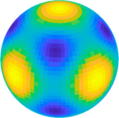
Figure 1. Gravitational potential on a sphere outside a cube. Note that the potential unit in this paper can be normalized as any value by Eq. 4.

2.2 Polyhedral method

For a polyhedral gravity field, the potential of a spacecraft at position r is (Werner and Scheeres, 1997):

$U\left(\mathbf{r}\right)=\frac{1}{2}G\sigma \left({\displaystyle \sum _{e\in \mathrm{e}\mathrm{d}\mathrm{g}\mathrm{e}\mathrm{s}}}{\mathbf{r}}_e\cdot {\mathbf{E}}_e\cdot {\mathbf{r}}_e\cdot L_e-{\displaystyle \sum _{e\in \mathrm{f}\mathrm{a}\mathrm{c}\mathrm{e}\mathrm{s}}}{\mathbf{r}}_f\cdot {\mathbf{F}}_f\cdot {\mathbf{r}}_f\cdot {\omega }_f\right)(4)$

where density $\sigma$ is assumed to be constant. Suffixes $e$ and $f$ denote the edge and face of the polyhedron. The face’s outward-pointing normal vector is ${\widehat{\mathbf{n}}}_f$, and its dyad ${\widehat{\mathbf{F}}}_f={\widehat{\mathbf{n}}}_f{\widehat{\mathbf{n}}}_f$ and ${\widehat{\mathbf{n}}}_e^f$ is outward edge normal perpendicular to both ${\widehat{\mathbf{n}}}_f$ and the edge. For the edge connecting vertices i and j shared by face A and B, the edge dyad is ${\widehat{\mathbf{E}}}_{ij}={\widehat{\mathbf{n}}}_A{\widehat{\mathbf{n}}}_{ij}^A+{\widehat{\mathbf{n}}}_B{\widehat{\mathbf{n}}}_{ji}^B$, with other similar definitions of ${\mathbf{E}}_e$s. If ${\mathbf{r}}_i$ is the vector form spacecraft to polyhedron vertex $P_i$, $r_i$ is its magnitude. $e_{ij}$ is the length between vertices $P_i$ and $P_j$; an edge factor $L_e$ is defined

$L_e={\int }_e\frac{1}{r}={\int }_{P_i}^{P_j}\frac{1}{r}\mathrm{d}s=\ln \frac{r_i+r_j+e_{ij}}{r_i+r_j-e_{ij}}.(5)$

${\omega }_f$ is a dimensionless face factor bounded by the triangular face $f$:

${\omega }_f=\int {\int }_{\text{triangle}}\frac{\mathrm{\Delta }z}{r^3}\mathrm{d}S=2\arctan \frac{{\mathbf{r}}_i\cdot {\mathbf{r}}_j\times {\mathbf{r}}_k}{r_i{r}_j{r}_k+r_i\left({\mathbf{r}}_j\cdot {\mathbf{r}}_k\right)+r_j\left({\mathbf{r}}_k\cdot {\mathbf{r}}_i\right)+r_k\left({\mathbf{r}}_i\cdot {\mathbf{r}}_j\right)}.(6)$

as the spacecraft’s gravitational acceleration is generally no longer on the radius directions for a non-spherical central body. In these calculations, some transformations are needed from spherical coordinates to Cartesian coordinates: $\tan \theta =y/x$, $\sin \varphi =z/r$, $r=\sqrt{x^2+y^2+z^2}$.

The polyhedral method can calculate gravity outside a celestial body, and it can also be used to calculate gravity near the surface on a celestial body; however, here we try to apply it to calculate the gravity on and inside the surface of a celestial body without much modification of its algorithm. This is one of the major contributions of this paper. Many examples and analysis will be given below.

3 Gravity field calculations around a cube or a rectangle

Unlike most existing literature, which gives gravitational comparisons between polyhedral and harmonic expansion methods by calculating the gravity on a cross-sectional plane, such as $x=0$, $y=0$, or $z=0$ (Werner and Scheeres, 1997) without the gravity inside the celestial bodies, this study calculates the gravity on a sphere. The reasons for this are that, firstly, that it is easy for comparative purposes, then for many practical missions whose orbit is near circular, such as gravity gradiometry satellites, and also for some algorithms such as the estimation of spherical harmonic coefficients. In this section, the calculation can be much simplified on a sphere.

For a homogenous cube whose dimension is $200\times 200\times$ 200 units of length, three spheres are special and typical both in geometry and gravity with radiuses of $R=100$, $R=100\sqrt{2}$, and $R=100\sqrt{3}$. There are figures in later sections, but here is a brief introduction. For the sphere $R=100\sqrt{2}$ intersecting the cube and also tangents to the eight edges of a cube, the parts of the cube near the eight corners of the cube are outside the sphere, and the other parts near the centers of the planes are inside the sphere. For the sphere $R=100\sqrt{3}$, the gravity examples can be seen in following section. It intersects the eight corner peaks of the cube and is also the smallest sphere completely outside the cube. The overall gravity patterns on the other larger spheres are quite similar. The sphere $R=100$ is tangential to the six flat surfaces at their centers, and it is also the largest sphere which is completely inside the cube. The gravities on these special spheres are calculated in this section, giving insights into the nature of the gravity around a cube. Before the calculation of gravity on these spheres, for convenience of comparison, the spherical harmonics coefficients of a cube and the gravity on its surface are calculated first.

Note that the acceleration unit in this paper can be normalized as any value. For example, if the length unit is kilometers, the density is about 1g/${\text{cm}}^3$ and the acceleration unit is mm/${\text{s}}^2$. We pay more attention to the relative value, which is the acceleration pattern and distribution about a cube.

3.1 The spherical harmonic coefficients around a rectangle

Due to the symmetry in a rectangle’s shape, the gravitational coefficients of its spherical harmonic expansion taken about its center of mass have a relatively simple form. First of all, $S_{lm}$ coefficients are identically equal to zero. Secondly, all coefficients $C_{lm}$ are such that either $l$ or $m$ are odd and are also equal to zero. Thus, the only non-zero gravity coefficients are those of the form $C_{2l,2m}$, $l,m=\mathrm{0,1,2},\dots$. Some explicit formula for the rectangle’s gravitational field coefficients are derived here, and the first few with the dimension 2a × 2b × 2c terms without normalization are specified as:

$C_{20}=\frac{1}{6r_0^2}\left(2c^2-a^2-b^2\right)(7)$

$C_{22}=\frac{1}{r_0^2}\left(a^2-b^2\right)(8)$

$C_{40}=\frac{1}{15r_0^4}\left(9a^4+9b^4+24c^4+10a^2{b}^2-40a^2{c}^2-40b^2{c}^2\right)(9)$

$C_{42}=\frac{1}{2r_0^4}\left(a^2-b^2\right)\left(10c^2-3a^2-3b^2\right)(10)$

$C_{44}=\frac{7}{r_0^4}\left(3a^2-b^2\right)\left(a^2-3b^2\right)(11)$

We can find that there is a similarity of the gravitational coefficients between a rectangle and an ellipsoid (Balmino, 1994; Scheeres, 2012), especially about $C_{20}=(2{\gamma }^2-({\alpha }^2+{\beta }^2))/(10r_0^2)$, $C_{22}=({\alpha }^2-{\beta }^2)/(20r_0^2)$ in the form of its semi-axis$(\alpha \ge \beta \ge \gamma )$. But other coefficients are different, there being no simple relation like $C_{40}=15/7(C_{20}^2+2C_{22}^2)$, $C_{42}=5/7C_{20}{C}_{22}$, $C_{44}=5/28C_{22}^2$ for an ellipsoid. It is obvious that for a cube$(a=b=c)$, $C_{20}=C_{22}=C_{42}=0$.

One simple way to calculate the spherical harmonic coefficients is to evaluate the gravity potential by Eq. 1 on a sphere outside the irregular central body using the polyhedral method. Then, by a usual least square algorithm, the coefficients can be obtained. See the compact form of the linear Eq. 12 about the coefficients. Since the $r$ in Eq. 1 is here a constant on a sphere, the calculation is simplified. This is one of the important reasons that we use spheres as calculating examples here–see the potential example on an exterior sphere in Figure 1. The larger potential (yellow) parts are directly above the center of the planes, and smaller potential (blue) parts are above the corners of the cube. The patterns show that the physical meaning is quite clear, which can justify the algorithm and the code to some degree. This is one reason why a cube has been chosen first for calculating examples in this paper. One drawback of this method is that outliers may appear in the results. For example, $S_{32}=-0.1777$ is not trivial when calculating $6\times 6$ coefficients, but $S_{54}=2.0173$ appears when calculating $8\times 8$ coefficients, and other coefficients are the same as in Table 1. It is unexpected that only one outlier exists for each of these two cases; however, because of this, it is easy to remove the outlier from the data. Luckily, the drawback of the results by this algorithm gives us a special strategy to remove the outlier.

$\left[\begin{array}{c}\hfill \dots \hfill \\ \hfill \frac{U\left(r,{\varphi }_i,{\lambda }_i\right)}{GM}-\frac{1}{r}\hfill \\ \hfill \dots \hfill \end{array}\right]={\left[\begin{array}{ccc}\hfill \dots \hfill & \hfill P_{10}\left(\sin {\varphi }_i\right)\hfill & \hfill \dots \hfill \\ \hfill \dots \hfill & \hfill P_{11}\left(\sin {\varphi }_i\right)\cos \left({\lambda }_i\right)\hfill & \hfill \dots \hfill \\ \hfill \dots \hfill & \hfill P_{11}\left(\sin {\varphi }_i\right)\sin \left({\lambda }_i\right)\hfill & \hfill \dots \hfill \\ \hfill \dots \hfill & \hfill P_{20}\left(\sin {\varphi }_i\right)\sin {\varphi }_i\hfill & \hfill \dots \hfill \\ \hfill \dots \hfill & \hfill P_{21}\left(\sin {\varphi }_i\right)\cos \left({\lambda }_i\right)\hfill & \hfill \dots \hfill \\ \hfill \dots \hfill & \hfill P_{21}\left(\sin {\varphi }_i\right)\sin \left({\lambda }_i\right)\hfill & \hfill \dots \hfill \\ \hfill \dots \hfill & \hfill P_{22}\left(\sin {\varphi }_i\right)\cos \left(2{\lambda }_i\right)\hfill & \hfill \dots \hfill \\ \hfill \dots \hfill & \hfill P_{22}\left(\sin {\varphi }_i\right)\sin \left(2{\lambda }_i\right)\hfill & \hfill \dots \hfill \\ \hfill \dots \hfill & \hfill \dots \hfill & \hfill \dots \hfill \\ \hfill \dots \hfill & \hfill P_{nm}\left(\sin {\varphi }_i\right)\cos \left(m{\lambda }_i\right)\hfill & \hfill \dots \hfill \\ \hfill \dots \hfill & \hfill P_{nm}\left(\sin {\varphi }_i\right)\sin \left(m{\lambda }_i\right)\hfill & \hfill \dots \hfill \end{array}\right]}^T\left[\begin{array}{c}\hfill \frac{r_0}{r^2}{C}_{10}\hfill \\ \hfill \frac{r_0}{r^2}{C}_{11}\hfill \\ \hfill \frac{r_0}{r^2}{S}_{11}\hfill \\ \hfill \frac{r_0^2}{r^3}{C}_{20}\hfill \\ \hfill \frac{r_0^2}{r^3}{C}_{21}\hfill \\ \hfill \frac{r_0^2}{r^3}{S}_{21}\hfill \\ \hfill \frac{r_0^2}{r^3}{C}_{22}\hfill \\ \hfill \frac{r_0^2}{r^3}{S}_{22}\hfill \\ \hfill \dots \hfill \\ \hfill \frac{r_0^n}{r^{n+1}}{C}_{nm}\hfill \\ \hfill \frac{r_0^n}{r^{n+1}}{S}_{nm}\hfill \end{array}\right](12)$

Table 1

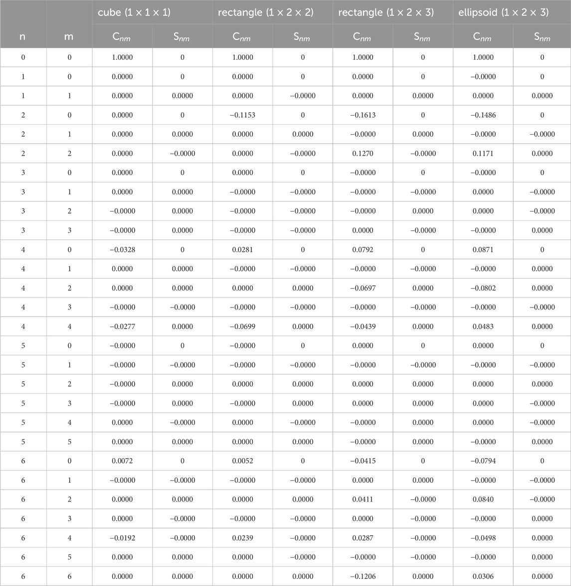
Table 1. Calculated normalized spherical harmonic gravity coefficients of a cube and rectangles to the order $6\times 6.$

The normalized spherical harmonic coefficient$(6\times 6)$, $C_{nm}$, shown in Table 1 together for comparison, are $S_{nm}$ from 0 to the order 6 by calculating a cube with a dimension $100\times 100\times 100$ length scale, and rectangles with the dimension $100\times 200\times 200$ and $100\times 200\times 300$, and also an ellipsoid whose semi-axes are $100\times 200\times 300$. It is interesting to see that only $C_{00},C_{40},C_{44},C_{60},C_{64}$ are not negligible for a cube ($200\times 200\times$ 200), $C_{20}$ appear also for a rectangle ($200\times 400\times$ 400), and $C_{22},C_{42},C_{62}$ appear also for a rectangle ($200\times 400\times$ 600), which can be validated by Eqs 7–11. It is evident that the number of a cube’s nontrivial coefficients is minimum except for a sphere. On the other hand, it also reveals the physical meaning of $C_{40},C_{44},C_{60},C_{64}$, etc., which represent the shape of a cube. Interested readers can also see a comparison of these coefficients to those of an ellipsoid with semi-axis ($100\times 200\times$ 300) length scale.

3.2 Gravity on the surface of a cube and a rectangle

Figures 2 and 3 visualize the total polyhedral gravity magnitudes on the surfaces of a cube and a rectangle. In Figure 3, one unexpected result is that the maximum gravity appears at a center of the mid-planes with the dimension $200\times 600$. This conclusion differs from the well-known result for an ellipsoid, whose maximum surface gravity appears at the end of its short axis while its minimum surface gravity is at the ends of its long axis (Guibout and Scheeres, 2003; Dobrovolskis, 2019). Figure 4 shows gravity on a cube in its surface direction, which could be helpful for understanding dust motion on surface. It is evident that near the edge, gravity is high but that it is zero at the center of the plane. The careful reader can find the largest tangential gravities appearing near the center of the edge. This gives some clue that a natural cube is rare in the celestial realm. All dust has a tendency to move to its surface center and accumulate to become a sphere. Some trajectory analysis is given in Section 4.2.

Figure 2

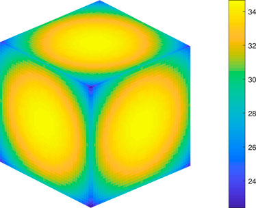
Figure 2. Total surface gravity.

Figure 3

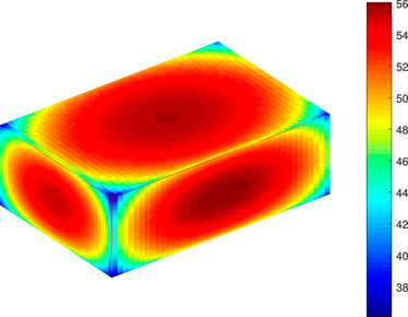
Figure 3. 3D surface gravity of a homogeneous rectangle by the polyhedral method.

Figure 4

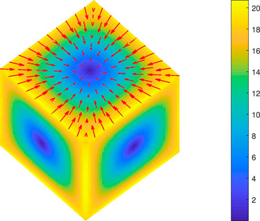
Figure 4. Gravity in surface direction.

3.3 Gravity on an intersecting sphere around the cube

Attention can be given to the special sphere with the radius $R=141.4$ of a cube with the dimension $200\times 200\times$ 200. In Figure 5, part of the sphere is tangential to the edge, and part of it is inside the corner or outside the plane center of the cube. Figure 6 shows the 2D map of the gravity of the cube on a sphere whose radius $R=141.4$ corresponds to the 3D Figure 5. Special attention should be given to the maxim gravity at the boundary line, which is both on the surface of the sphere and the cube. In this figure, the larger value appears at the middle of each edge of the cube, tangential to the sphere. The yellow boundary around the corners of the cube is also on its surface. Inside the boundary near the corners, the gravity is inside the corners of the cube, which is smaller than the corresponding boundary with same radius on the surface. This is physically correct. This also shows that the polyhedron algorithm works well for all these different cases. Hence, we visualize the gravity inside the cube, which could be helpful for understanding internal structure and the evolution of a celestial body. This sphere includes parts both inside the corner and outside the central plane of the cube. It is obvious for the outside parts of the sphere above the planes of the cube that its gravity is also smaller than the gravity on the boundary both on the surface of the cube and of the sphere. This is good example of how the polyhedral method is not only valid for the gravitational calculation outside a solid body but also works well for the place inside or on its surface; relatively very few researchers have done it this way. The harmonic expansion method only works for the spheres far enough from its central body. Again, we note that the acceleration unit in this paper can be normalized as any value. For example, if the length unit is kilometers, density is about 1g/${\text{cm}}^3$ and the acceleration unit is mm/${\text{s}}^2$. Here, we pay more attention to the relative value–the acceleration pattern and distribution about a cube.

Figure 5

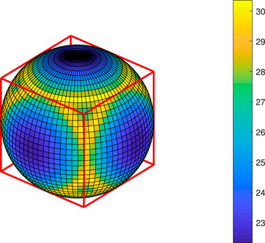
Figure 5. 3D gravity of a cube on a sphere with radius $R=141.4$.

Figure 6

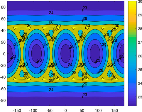
Figure 6. 2D contour map of gravity in Fig.5, longitude vs. latitude (deg).

3.4 Gravity on a sphere outside the cube

For this, see Figures 7–9. For even larger spheres outside the cube, their overall gravitational patterns are all similar. Interested readers can compare Figure 7 to Figure 1, in that the place (above corner of the cube) on the sphere of larger gravity corresponds to the place with smaller potential, whereas the place (above the center of a plane) of smaller gravity corresponds to the place with larger potential on the sphere. Thus, the place on the sphere with larger potential is at the same place with smaller gravity, and vice versa is compatible with the general definitions of potential and gravity. Particularly in Figure 9, the overall error is acceptable, and largest errors appear near the corner of the cube at about 10%. The error in the large yellow part is very small. The accuracies can be improved even further by adding more spherical harmonic terms in the model, such as $C_{60},C_{64},C_{80},C_{84},C_{88}$.

Figure 7

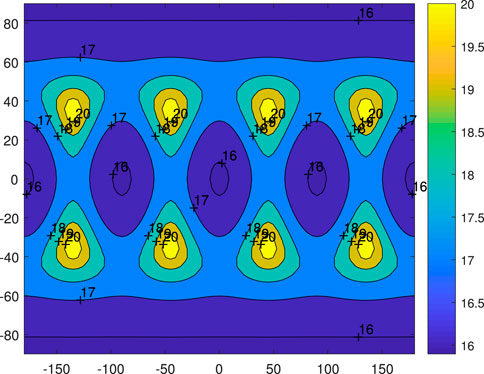
Figure 7. Gravity of polyhedron model for a cube at a sphere of radius$R$ = 175.

Figure 8

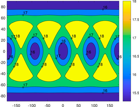
Figure 8. Gravitational field of 4^th degree and order spherical harmonic expansion for cube on a sphere of radius 175, which is just outside the cube.

Figure 9

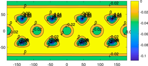
Figure 9. Comparison of the gravity between spherical harmonics and polyhedral model, $(G_{sh}-G_{\mathit{poly}})/G_{\mathit{poly}}$ when $R=175$.

3.5 Gravity inside the cube

The polyhedral method is again applied to investigate the gravity inside a celestial body, which is closely related to the internal stress and strain. This kind of research is helpful for analyzing the internal structure and evolution of an asteroid. The gravity on a sphere $r=100$, which is just inside the cube, is calculated. See Figure 10 and compare with Figure 2 ,which is similar in overall pattern; the maximum value appears just at the center of each plane of the cube. For other even smaller spheres, the gravitational configurations on them are all similar. However, the errors calculated by spherical harmonics are all too large, especially near the corners (Figures 11, 12). We see that the errors are totally unacceptable for the spherical harmonic expansion method, especially near the corners of the cube. The relativity is up to 200–300%. Interior spherical harmonic coefficients are needed (Takahashi et al., 2013). With this situation, some special modifications for this method should be given (Takahashi et al., 2013; Scheeres, 2012; Pearl et al., 2018; Arora and Russell, 2012).

Figure 10

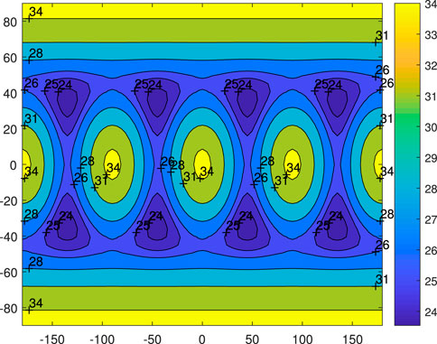
Figure 10. Gravitational acceleration of polyhedral model for cube at $R=100$ distance.

Figure 11

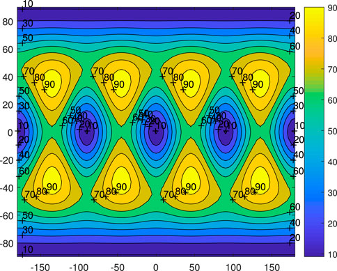
Figure 11. Gravitational field of 4^th degree and order spherical harmonic expansion on sphere with radius 100 which is just completely inside the cube.

Figure 12

Figure 12. Comparison of gravity between spherical harmonics and polyhedral model, $(G_{sh}-G_{\mathit{poly}})/G_{\mathit{poly}}$ when $R=100$.

4 Application examples

4.1 Near circular orbit

With the polyhedral model, spacecraft landing and ascending trajectories can be calculated, but more interesting theoretical results can be obtained if secular motion is studied. The secular motion of periapsis in the orbital tori is similar to the well-known Mercury apsidal secular perturbation motion around the Sun. See Figures 13 and 14 and consider an initial circular orbit $e=0$ in the equatorial plane $i=0$; it can be seen that the semi-major axis $a$, eccentricity $e$, and inclination $i$ are constant on average, the longitudinal of the ascending node $\mathrm{\Omega }$ increases, and the argument of periapsis $\omega$ decreases by averaging the true anomaly $\nu$. The $\mathrm{\Omega }$’s rate is just twice the rate of $\omega$, which can be explained by Eqs 13;–;16; the corresponding curves are on Figure 14. The orbit moves 16 periods, whereas the longitude processes only one period in about 350 time units. This can be derived without difficulty for the averaged equation of six elements using classical averaging theory (Kaula, 1966):

$\dot{a}=\dot{e}=\dot{i}=0(13)$

$\dot{\mathrm{\Omega }}=-\frac{35C_{40}n\cos i}{8p^4}\left[\left(6/7+9/7e^2\right)-\left(3/2+9/4e^2\right){\sin }^{2}i\right],(14)$

$\dot{\omega }=\frac{35C_{40}n}{8p^4}\left[\left(12/7+27/14e^2\right)-\left(93/14+27/4e^2\right){\sin }^{2}i\right.(15)$

$\left.+{\sin }^{4}i\left(21/4+81/16e^2\right)\right].$

Figure 13

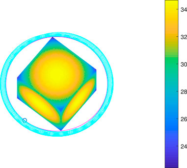
Figure 13. Example orbit around a cube with initial orbit in equatorial plane, calculated by polyhedral model.

Figure 14

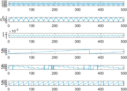
Figure 14. From top to bottom, calculated classical six elements for the orbit in Figure 13: $a$, $e$, $i$, $\mathrm{\Omega }$, $\omega$, $\nu$. The unit for angles are deg. Pay more attention to the trend of variation.

Short period oscillation is mainly due to the term $C_{44},C_{64}$. In Figure 14, from top to bottom, the calculated classical six elements for the orbit in Figure 13 are semi-major axis $a$, eccentricity $e$, inclination $i$, longitude of ascending node $\mathrm{\Omega }$, argument of periapsis $\omega$, and true anomaly $\nu$. The unit for angles are degrees. More attention should be paid to the trend of variation.Other researchers are also interested in the orbital motion around a cube (Liu et al., 2011), which shows a few families of periodic orbits.

4.2 Motion on a surface

Figure 15 shows three examples of motion: a particle moving without friction in a straight line (green), a circle (red), and a general tori trajectory (blue) on a surface of a cube via polyhedral gravity calculations. When there is no initial lateral velocity, the dust or a cart’s motion is on a straight line (green line), like a spring’s harmonic motion. With the proper choice of lateral velocity, the motion can be in a periodic trajectory, similar to a circle (red circle). A random velocity normally leads to a tori trajectory (blue trajectory). The only forces acting on the particle are the gravity from the cube and the supporting force out of the surface. No friction is assumed here.

Figure 15

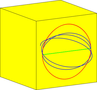
Figure 15. Particle on surface moving without friction in a straight line (green), a circle (red), a general tori trajectory (blue).

For a cube with dimension $2\times 2\times 2$ unit length, the motion is simple with initial condition $x_0=0.9$, $z_0=0$ in the plane $y_0=1$. Even for this simple case, a complete proof is also tedious as too many terms should be included. A simplified analysis is here given. In gravity, these kinds of terms appear by simple formulation.

$r_i=\sqrt{x^2+2x+6}(16)$

$r_j=\sqrt{x^2-2x+6}(17)$

$k=-\frac{r_i+r_j}{r_i{r}_j\left({\left(r_i+r_j\right)}^2-4\right)}(18)$

$b=-\frac{r_i-r_j}{r_i{r}_j\left({\left(r_i+r_j\right)}^2-4\right)}(19)$

$\ddot{x}=kx+b(20)$

Where the length of the cube is 2, $r_i,r_j$ is the distance from the attracted mass point to the corners of the adjacent corners $i,j$ of the related edge. It is easy to show that $|b/k|\ll 1$ (less than 10%) and $k$ is almost a constant when $-1<x<1$. It is only near the edge that a little nonlinear property appears. The motion is then similar to mass spring harmonic motion. These accelerations can also be seen in the arrow representations in Figure 3 for both direction and magnitude.

When friction exists, the tori and circle motion become spiral. The linear oscillation’s amplitude will dwindle. Finally, all the motions will be stopped at the center of the plane. This could be an explanation of why in the natural world a pure cube celestial body with sharp corners is rare.

5 Discussion and Conclusion

There is already some literature discussing the gravity of Asteroid 4,769 Castalia, original data of which can be found in Hudson and Ostro (1994). Here we show a different figure (Figure 16) which calculates and visualizes the surface gravity without centrifugal force resulting from rotation for theoretical comparison. More practical calculations about this irregularly shaped asteroid’s surface gravity, internal gravity, and slope with rotation can be found in our newly published paper (Hu et al., 2024). To theoretically understand the nature of gravity of different shapes by different methods, gravitational calculations are performed for a cube, but on its surface and different spheres around it by polyhedron and harmonic expansion methods for different cases. In these examples, a few different perspectives of these methods and results are revealed, such as the maximum gravity being at the plane’s centers and the minimum at the corners on the surface. For a sphere that intersects the cube, the maximum gravity is on the intersection between the cube and the sphere. This means that on the sphere, the gravities inside and outside the cube are smaller than the gravity on the intersection—that on the surface of the cube. If high-order coefficients of harmonic expansion are calculated for a cube, nontrivial terms are such as $C_{40},C_{44},C_{60},C_{64},C_{80},C_{84},C_{88},C_{100},C_{104},C_{108}$. From another point of view, this reveals the physical meaning of these terms in spherical harmonic expansions. These analyses are extended to rectangles; for a general rectangle, the maximum gravity appears at the center of its mid-plane, and for its harmonic expansion coefficients such as $C_{20},C_{22},C_{42},C_{62}$, $C_{66},C_{82},C_{86},C_{102},C_{106},C_{1010}$, terms also appear.

Figure 16

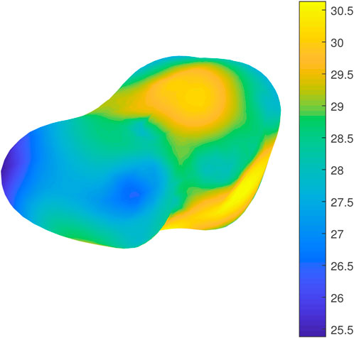
Figure 16. Gravitational acceleration on surface of asteroid 4,769 Castalia without rotation, unit:$10^{-2}$mm/${\text{s}}^2$.

It can be seen in Figure 16 that the asteroid can be approximated to two connected cubes with smooth corners. The local maximum surface gravity appears near the centers of the planes, and local minimum gravity is at the corners of the cube, which is compatible with the analysis of a rectangle’s gravity here.

Hence, in this study a cube’s gravity is focused, as its gravity acceleration distribution is regular, simple, and fundamental. These results could be interesting for readers in widely different research areas, just like an ellipsoid’s gravity which is also convenient for comparison—see the effective surface gravity slope in Figure 17, which differs from Figure 10 in Dobrovolskis (2019). In this paper, ${\omega }_{ab}<{\omega }_{ac}<{\omega }_{bc}$, which seems more reasonable. The definition of the effective gravity slope is the same—the angle from minus normal of the surface to its local effective gravitational direction. Especially note that if the gravity slope at some spot is larger than 90° then dust on it is flying off or shedding away from the ellipsoid, just as at the end of the long axis in subplot 8. The ellipsoid in subplot 1 does not rotate. In subplot 2, its angular velocity is ${\omega }_{ab}$; for subplot 5, ${\omega }_{ac}$; subplot 7, ${\omega }_{bc}$, as defined in Dobrovolskis (2019); that is, ${\omega }_1=0<{\omega }_2={\omega }_{ab}<{\omega }_3<{\omega }_4<{\omega }_5={\omega }_{ac}<{\omega }_6<{\omega }_7={\omega }_{bc}<{\omega }_8$.

Figure 17

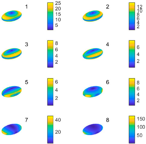
Figure 17. Effective gravity slope (deg) on rotating ellipsoid with angular velocity increasing from left to right and then from top to bottom, as the sequence subplot 1-8.

Data availability statement

The original contributions presented in the study are included in the article/Supplementary Material; further inquiries can be directed to the corresponding author.

Author contributions

WH: Funding acquisition, Investigation, Methodology, Writing–original draft. TF: Validation, Writing–review and editing. YW: Funding acquisition, Validation, Writing–review and editing.

Funding

The authors declare that financial support was received for the research, authorship, and/or publication of this article. This work was supported by the National Natural Science Foundation of China under Grant 11872007 and the Fundamental Research Funds for the Central Universities.

Conflict of interest

The authors declare that the research was conducted in the absence of any commercial or financial relationships that could be construed as a potential conflict of interest.

Publisher’s note

All claims expressed in this article are solely those of the authors and do not necessarily represent those of their affiliated organizations, or those of the publisher, the editors and the reviewers. Any product that may be evaluated in this article, or claim that may be made by its manufacturer, is not guaranteed or endorsed by the publisher.

References

Balmino, G. (1994). Gravitational potential harmonics from the shape of an homogeneous body. Celest. Mech. Dyn. Astronomy 60, 331–364. doi:10.1007/bf00691901

CrossRef Full Text | Google Scholar

Banerjee, B., and Buddhadeb, S. (1977). Gravitational attraction of a rectangular parallelepiped. Geophysics 42 (5), 1053–1055. doi:10.1190/1.1440766

CrossRef Full Text | Google Scholar

Bannister, M., Bhandare, A., Dybczyński, P. A., Fitzsimmons, A., Guilbert-Lepoutre, A., Jedicke, R., et al. (2019). The natural history of oumuamua. Nat. Astron. 3 (7), 594–602. doi:10.1038/s41550-019-0816-x

CrossRef Full Text | Google Scholar

Chappel, J., and Abbott, A. I. D. (2012). The gravitational field of a cube. Class. Phys. 2015, 1–10.

Google Scholar

Dobrovolskis, A. (2019). Classification of ellipsoids by shape and surface gravity. Icarus 321, 891–928. doi:10.1016/j.icarus.2018.11.023

CrossRef Full Text | Google Scholar

Fukushima, T. (2017). Precise and fast computation of the gravitational field of a general finite body and its application to the gravitational study of asteroid eros. Astronomical J. 164 (4), 145. doi:10.3847/1538-3881/aa88b8

CrossRef Full Text | Google Scholar

Guibout, V., and Scheeres, D. (2003). Stability of surface motion on a rotating ellipsoid. Cel.Mech. Dyn. Astron 87 (3), 263–290. doi:10.1023/b:cele.0000005720.09027.ee

CrossRef Full Text | Google Scholar

Herrera, E., Palmer, P., and Roberts, R. M. (2013). Modeling the gravitational potential of a nonspherical asteroid. J.of GCD AIAA 36 (3), 790–798. doi:10.2514/1.58140

CrossRef Full Text | Google Scholar

Hu, W. (2015). Fundamental spacecraft dynamics and control. John Wiley and Sons.

Google Scholar

Hu, W., Fu, T., and Liu, C. (2024). Revisiting the numerical evaluation and visualization of the gravity fields of asteroid 4769 castalia using polyhedron and harmonic expansions models. Appl. Sci. 14 (10), 4058. doi:10.3390/app14104058

CrossRef Full Text | Google Scholar

Hu, W., and Scheeres, D. (2002). Spacecraft motion about slowly rotating asteroids. J. GCD AIAA 25 (4), 765–775. doi:10.2514/2.4944

CrossRef Full Text | Google Scholar

Hu, W., and Scheeres, D. (2004). Numerical determination of stability regions for orbital motion in uniformly rotating second degree and order gravity fields. Planet. Space Sci. 52 (8), 685–692. doi:10.1016/j.pss.2004.01.003

CrossRef Full Text | Google Scholar

Hu, W., and Scheeres, D. (2014). Averaging analyses for spacecraft orbital motions around asteroids. Acta Mech. Sin. 30 (3), 294–300. doi:10.1007/s10409-014-0050-9

CrossRef Full Text | Google Scholar

Hudson, R., and Ostro, S. (1994). Shape of asteroid 4769 castalia (1989 PB) from inversion of radar images. Science 263, 940–943. doi:10.1126/science.263.5149.940

PubMed Abstract | CrossRef Full Text | Google Scholar

Kaula, W. (1966). Theory of satellite geodesy. Waltham, MA: Blaisdel, 1–11.

Google Scholar

Liu, X., Baoyin, H., and Ma, X. (2011). Equilibria, periodic orbits around equilibria, and heteroclinic connections in the gravity field of a rotating homogeneous cube. Astrophys Space Sci 333 (2), 409–418. doi:10.1007/s10509-011-0669-y

CrossRef Full Text | Google Scholar

MacMillan, W. (1958). The theory of the potential. New York: McGraw-Hill. Republished by Dover.

Google Scholar

Michalodimitrakis, M., and Bozis, G. (1985). Bounded motion in a generalized two-body problem. Astrophys. Space Sci. 117 (2), 217–225. doi:10.1007/bf00650148

CrossRef Full Text | Google Scholar

Mysen, E., Olsen, O., and Aksnes, K. (2006). Chaotic gravitational zones around a regularly shaped complex rotating body. Planet. Space Sci. 54 (8), 750–760. doi:10.1016/j.pss.2006.04.005

CrossRef Full Text | Google Scholar

Nagy, D. (1966). Gravitational attraction of a right rectangular prism. Geophysics 31, 262–371.

CrossRef Full Text | Google Scholar

Nikolaeva, E., Starinova, O., Shornikov, A., and Chernyakina, I. (2019). “Ballistic and design of nano-class spacecraft for asteroid exploration,” in 9th International Conference on Recent Advances in Space Technologies (RAST) (Istanbul, Turkey: IEEE), 89–94.

CrossRef Full Text | Google Scholar

Parikh, D., and Tewari, A. (2021). Optimal landing strategy on a uniformly rotating homogeneous rectangular parallelepiped. J. Astronautical Sci. 68, 120–149. doi:10.1007/s40295-020-00243-y

CrossRef Full Text | Google Scholar

Pearl, J., Louisons, W., and Hitt, D. L. (2018). “Hybrid gravity model from asteroid surface topology,” in AIAA Space Flight Mechanics Meeting, Florida USA, 8–12 January 2018. doi:10.2514/6.2018-0955

CrossRef Full Text | Google Scholar

Pinson, R., and Lu, P. (2019). Trajectory design employing convex optimization for landing on irregularly shaped asteroids. AIAA J. Guid. Control Dyn. 41 (6), 1243–1256. doi:10.2514/1.g003045

CrossRef Full Text | Google Scholar

Russell, R. P., and Arora, N. (2012). Global point mascon models for simple, accurate, and parallel geopotential computation. Journal of Guidance Control and Dynamics 35 (5), 1568–1581. doi:10.2514/1.54533

CrossRef Full Text | Google Scholar

Scheeres, D. (2012). Orbital motion in strongly perturbed environments. UK: Springer.

Google Scholar

Scheeres, D., Ostro, S., Hudson, R., and Werner, R. (1996). Orbits close to asteroid 4769 castalia. Icarus 121 (1), 67–87. doi:10.1006/icar.1996.0072

CrossRef Full Text | Google Scholar

Sebera, J., Bezdek, A., Pešek, I., and Henych, T. (2016). Spheroidal models of the exterior gravitational field of asteroids bennu and castalia. Icarus 272, 70–79. doi:10.1016/j.icarus.2016.02.038

CrossRef Full Text | Google Scholar

Takahashi, Y., Scheeres, D., and Werner, R. A. (2013). Surface gravity fields for asteroids and comets. AIAA J. Guid. Control Dyn. 36 (2), 362–374. doi:10.2514/1.59144

CrossRef Full Text | Google Scholar

Valvano, G., Winter, O., Sfair, R., Machado Oliveira, R., Borderes-Motta, G., and Moura, T. S. (2022). Apophis - effects of the 2029 earth’s encounter on the surface and nearby dynamics. Mon. Notice R. Astronomical Soc. 510 (1), 95–109. doi:10.1093/mnras/stab3299

CrossRef Full Text | Google Scholar

Venditti, F., and Prado, A. (2019). Mapping orbits regarding perturbations due to the gravitational field of a cube. Math. Problems Eng. 2015, 1–11. doi:10.1155/2015/493903

CrossRef Full Text | Google Scholar

Waldvogel, J. (1976). The Newtonian potential of a homogeneous cube. J. Appl. Math. Physics(ZAMP) 27, 867–871. doi:10.1007/bf01595137

CrossRef Full Text | Google Scholar

Werner, R. (1994). The gravitational potential of a homogeneous polyhedron or don't cut corners. Mech. Dyn. Astron 59 (3), 253–278. doi:10.1007/bf00692875

CrossRef Full Text | Google Scholar

Werner, R., and Scheeres, D. (1997). Exterior gravitation of a polyhedron derived and compared with harmonic and mascon gravitation representations of asteroid 4769 castalia. Celest. Mech. Dyn. Astronomy 65 (3), 313–344. doi:10.1007/bf00053511

CrossRef Full Text | Google Scholar