Modeling the influence of an electric thruster’s ion beam on its global EMC

This research deals with electromagnetic compatibility (EMC) in the field of electric propulsion (EP). To complete previous investigations, the emissions of a fully operating radio-frequency thruster (RIT)—including its extracted ion beam—were numerically analyzed. The ion beam was simulated and investigated with various characteristics. The simulations were performed by means of transient co-simulation. It is clear that the ion beam had a significant impact on the thruster emissions. Properties such as divergence angle and the conductivity of the beam, which can be directly attributed to the operating point of the plasma discharge inside the thruster, play a major role. The next steps will be to bring together all the knowledge gained about the emissions of the individual thruster components as well as the peripheral electronics.

1 Introduction

Traditionally, electric thrusters have been primarily used for station-keeping and orbit attitude control missions. Nowadays, electric thrusters are also used as propulsion systems for orbit raising and space travel. Increasing commercialization has a great impact on space flight—especially on electric propulsion systems. Scientific, political, military, and economic goals present strong reasons for the emerging demand for space flight. The challenges that still exist are leading to extensive research in areas such as energy efficiency, electromagnetic compatibility, alternative propellants, and scalability (Holste et al., 2020).

Electromagnetic compatibility (EMC) is “the ability of an equipment or system to function satisfactorily in its electromagnetic environment without introducing intolerable electromagnetic disturbances to anything in that environment” (International Electrotechnical Commission, 2018). Spacecraft EMC technology is based on traditional theory but is further complicated by weight, reliability, the space environment, and cost requirements. Since spacecraft are typically subject to various operating conditions, such as integration testing, launch, and on-orbit operation, special attention should be paid to the impact of these conditions on the electromagnetic environment (EME). Therefore, the EMC characteristics of the spacecraft are related to its EME (Zhang et al., 2021). To meet these requirements, a holistic understanding of the EMC of a thruster assembly is required. Some parts of the thruster assembly have been analyzed separately. In past studies, for example, a radio-frequency generator was investigated for its EMC by simulation and measurement (Rover and Volkmar, 2022). It became clear that the supply lines and cabling to the thruster are the decisive influencing factors from an EMC point of view. Furthermore, a semi-anechoic vacuum chamber was designed and set up at our department and is described in a previous publication (Rover et al., 2023). There seem to be no recent studies or substantial research results related to the electromagnetic interference (EMI) of an ion beam.

The device tested was a radio-frequency ion thruster, where the designation RIT-4 indicates the 4-cm diameter of the grid extraction system. We have analyzed and reported here the influence and EMI characteristics of the thruster, including its extracted ion beam, in order to complete the investigation of individual thruster areas. We also validated the general use of the simulation environment.

The motivation of this research is presented in Section 2. Section 3 describes the environment of the simulation where the thruster and the ion beam were examined. Additional features and model characteristics are introduced in Section 4. Section 5 shows the validity of the simulation environment, and thus the accuracy of the results, using physical principles and mathematical analyses. Results and comparisons of different operating points are presented in Section 6, including best practice. Finally, Section 7 summarizes the work and its outputs and provides an outlook.

2 Motivation

Ion thrusters, which are an essential part of “NewSpace” missions, play an important role in spacecraft propulsion and maneuvering systems. These thrusters and their peripherals must therefore be safe and reliable. In addition to functionality, electromagnetic compatibility requirements must be met to ensure stable operation under all operating conditions. Furthermore, the mutual interference of active high-frequency components—such as the radio-frequency generator typically used in RF ion thrusters—and satellite components must be taken into account in terms of immunity and emissions. Electronics comprise about 60% of the total thruster assembly, which indicates the importance of studying these supposedly “peripheral” components and their interaction with the thruster and other satellite components.

3 Simulation approach

The simulation consisted of a 3D model and an electrical circuit, called schematic in the simulation process. The 3D model represented the physical conditions of the object under investigation. The schematic generated and fed the supply signals as well as further electrical elements.

The simulation was performed with SIMULIA CST Studio Suite software version 2023 SP5 from $DassaultSyst\grave{e}mes$. A full-wave 3D electromagnetic simulation was performed in order to increase the predictability of the radiated emissions of the system during different operating conditions. In this type of simulation, all Maxwell equations are solved without any simplifying assumptions. The 3D model consisted of mechanical components such as the thruster itself as well as models of the discharge plasma and extracted ion beam. The neutralizer was an important part of the thruster and its operation. In this research, it was disregarded because the resulting electron cloud is diffuse, and, therefore, a simple first-order model is not sufficiently concrete. Accordingly, only the ion beam was first characterized, providing sufficient accuracy for the model. During the ground tests in our laboratories, the setup was also often operated without a neutralizer; we thus had a first comparable indicator with the model. However, any realistic space scenario would dictate the use of a neutralizer. Therefore, this research should be understood as a first step toward a holistic EMC simulation approach.

The electronic components and control signals are defined in the schematic tab. The combination of these two types of modeling produces a transient co-simulation—an alternative to the standard simulation. The standard process uses S-parameters to describe the 3D model for any combination of port excitations. Their calculation requires either a frequency sweep (frequency-solver) or a simulation per port (time-solver). In transient co-simulation, on the other hand, only one simulation of the coupled circuit is performed, where the excitation is defined in the schematic tab. Fortunately, the 3D model and the schematic were solved simultaneously, so interactions and mutual influences between the 3D model and the schematic were taken into account. In the standard simulation, however, S-parameters are first derived from the 3D model and are then linked to the schematic part. Accordingly, the transient co-simulation was used.

In conducted disturbances, the near and far field are important quantities within EMC. These areas can be addressed with the model shown. Here, the individual case of the far field and the interaction and effect of the thruster and extraction beam were explored to complete the previous research. To obtain the simulated far-field electrical characteristics, it was necessary to place field monitors and field probes at the desired distance from the model (source). Their position depended on the desired frequency range as well as the desired accuracies. In this project, a frequency range of 0–1 GHz was considered. Above 30 MHz, the radiated disturbances usually dominate the conducted disturbances (European cooperation for space standardization, 2012), so we focused on the radiation’s impact on the results. As field probes monitored the radiated powers, post-processing allowed calculation of the electrical field strengths of the far field. Transient signals defined in the schematic excited the 3D model, and signal type, amplitude, and frequency could be set.

Post-processing calculations as well as the defining shape and spatially resolved conductivity of the ion beam were performed using MATLAB software version R2022a from The MathWorks, Inc. The basis of the beam conductivity calculation is the distribution function of the ions; their relevant descriptive parameters depend on assumptions of grid and plasma properties. According to Figure 1, the ion beam consisted of volume elements that model the beam shape and allow spatially resolved individual conductivity settings. If the parameters changed, the ion beam was recalculated.

FIGURE 1

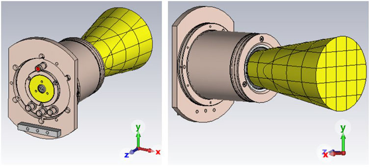
FIGURE 1. Modeling of RIT-4 and ion beam.

The model permitted us to test various operating points of the thruster and obtain the radiation characteristics of the thruster with an active ion beam. This enabled preliminary checks to be made on the EMC behavior of a fully operating thruster at specific operating points.

4 Modeling

4.1 3D model

The 3D model included the RIT-4, the plasma, and also the ion beam (Figure 1). The RIT-4 model and the plasma modeling had been set up in a previous work (Baruth, 2017); the dimensions and materials were defined and assigned to its components. In order to consider the plasma from an electrotechnical point of view, its dielectric properties were determined. For this purpose, a Drude plasma was used (Chabert and Braithwaite, 2011). In the simulation model, a material with the appropriate dielectric properties could be created and placed in the interior of the ionization vessel to mimic the behavior of a real plasma to a certain extent— sufficiently accurate for EMC analyses. The plasma conductivity mainly depended on these parameters:

• electron plasma frequency ω_pe (with electron density n_e),

• effective impact frequency v_m,eff,

• excitation frequency ω.

These parameters can be determined by simulation or experiment. However, this requires self-consistent models that are specifically tailored to low-temperature plasmas. The determination was carried out in Baruth (2017).

4.2 Ion beam

The ion beam was also represented by materials of different conductivities. First, the density was calculated based on the spatial distribution of the ions inside the beam. As can be seen in Figure 2, the density number decreases along the ion beam with the square distance to the extraction grid, as in Eq. 1:

$\rho \propto \frac{1}{z^2}.(1)$

FIGURE 2

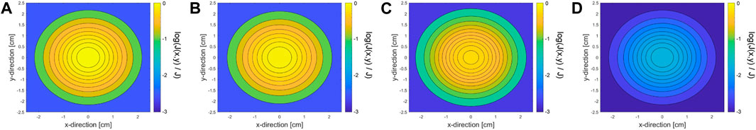
FIGURE 2. Normalized ion density distribution in the x–y plane at varying axial distance downstream from the thruster grid: (A) at the extraction grid, (B) at 1/3 length of the ion beam, (C) at 2/3 length of the ion beam, (D) at the end of the simulated ion beam.

The location-dependent densities J (x, y) and J(z) are related to total density J on the grid. From the center of the beam, the density decreases outward according to a Gaussian profile. The application of the Gaussian profile is also subject to boundary conditions: the far-field condition approximates the representation of the current density by a plane wave. The standard deviation in the far field of the ion distribution is determined by Eq. 2:

$\sigma =\frac{z}{2.4477}\cdot \tan \alpha .(2)$

Here, σ is the standard deviation, z the ion beam length, and α the divergence angle. A value of 2.4477 follows from the calculation of the chi-square distribution of second degree (Reynolds, 1971). Another condition is keeping a certain ratio of the beam length to the radius R₀ of the extraction grid to ensure far-field beam conditions, as in Eq. 3:

$\frac{z}{R_0}=6\dots 8.(3)$

Eqs 4, 5 were used to calculate the current density J and conductivity κ:

$J=\frac{I}{A}=q\cdot n\cdot v,(4)$

$\kappa =\frac{J\cdot z}{V}.(5)$

Here, J is the current density, I the ion beam current, A the grid area, κ the conductivity, and V the high voltage at the extraction grids. The current density was calculated for the grid area. Due to the ion distributions in the z-direction and in the x–y plane (Figure 2), the current density was adjusted by the distribution functions at the further positions in the ion beam.

When determining the current, the charge of a single ionized xenon particle is q = 1e = 1.602 ⋅ 10^–19 As and its mass is m = 131.293 u with mass unit u = 1.66054 ⋅ 10^–27 kg. It is assumed to be constant, as well as the velocity v, which depends on the grid voltage V according to Eq. 6:

$v\approx \sqrt{\frac{2\cdot q\cdot V}{m}}.(6)$

With V = 1 kV, the velocity is v ≈ 38.335 km/s.

There are a number of state-of-the-art modeling approaches with corresponding tools for simulating ion optics. The limitation of computing power led to the electrons being calculated with the Boltzmann relation (fluid) and not as particles (PIC approach), and only one beamlet was simulated (Becker and Herrmannsfeldt, 1992; Kalvas et al., 2010; Reeh et al., 2017). There are approaches to simulating the entire extraction system including the beam; very large computational requirements (computational clusters) are necessary because there is insufficient information about the actual beam. The current beam profile depends on the curvature of the grids and also on the plasma density distribution in the ionization vessel (Dobkevicius and Feili, 2016; Reeh et al., 2019). The model is based on empirical values. We thus used a first-order model that can also commonly be found in the literature (Goebel and Katz, 2008) and that could be validated in empirical experiments (Scholze et al., 2019).

First, cubes of equal size were generated, each assigned to a material with individual calculated conductivity. Then, a cone shape was formed using the divergence angle. The ion beam was created when the cone shape and cubes overlapped. The better the discretization, the more accurate the replication. For reasons of low calculation time and project size, a discretization of five steps per axis was used. Accordingly, there were up to 125 cubes to model the ion beam (Figure 1). Using an application programming interface (API), the ion beam was created directly with MATLAB commands in the CST environment. The API (Symeonidis, 2018) used was extended with modified methods and new functionalities, such as setting project properties, creating shapes, and combining materials and shapes.

4.3 Electronics and control

The schematic tab represents the electrical components and control system (Figure 3). The RFG drive signal was a square wave with a given frequency and maximum value. A capacitance was connected, which completed the actual resonant circuit. The value of 2.27 nF was chosen because of a known and used RFG; a realistic value for a coil inductance of the RIT-4 is 1.2 μH. Using Eq. 7, the optimum excitation frequency is calculated:

$f=\frac{1}{2\cdot \pi \cdot \sqrt{L\cdot C}}.(7)$

FIGURE 3

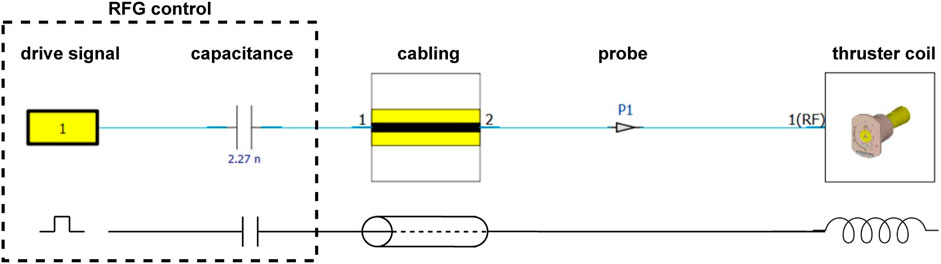
FIGURE 3. Schematic tab of the simulation with illustrative symbols.

A cable simulation was also included. The cable was located between the output circuit of the control and the coil port of the RIT-4 model. The cable simulation included geometric data of the triaxial cable used. The length was set to 0.65 m. All other data such as the material of the conductor or insulation are given according to the data sheet of the cable type Belden 9,222 Triax.

5 Verification

The goal of verification is to check the simulation results using analytical equations. To ensure the validity of the simulation, a known and computable antenna structure is modeled: the Hertzian dipole. It is used to calculate the electric far field at a given distance r by applying an analytical equation. First, this equation was derived. Second, the simulation software CST was used to simulate the dipole structure. Its results were compared with the analytical solution.

The Hertzian dipole is a fictional construct intended to simulate two oscillating point charges; the theoretical equations for electric fields are derived from it. Accordingly, this construct can represent any electrical far-field situation. From an electromagnetic point of view, every structure acts like three orthogonal dipoles (Figure 4). The design, size, and excitation of each dipole depend on the situation describing the emissions; they are independent of each other. The ideal Hertzian dipole is an infinitesimal short current element, which generates the same radiation as an electrically long wire, such as with l = λ/2. At integer multiples of λ/2, the radiation is maximal (Kark, 2016). Thus, it is a theoretical construct that enables validation of the solver and the simulation; a possible replica is shown in Figure 5. For structures of length dl, traversed by alternating current i and frequency f, the electric field strength is calculated according to Eq. 8, depending on the distance r to the dipole (in main radiation direction) (Gustrau, 2015):

$\mathrm{d}{E}_{\text{max}}\approx \mathrm{d}{E}_{\mathrm{\theta }}=Z_0\cdot \frac{i\cdot \mathrm{d}l\cdot f}{2\cdot c_0\cdot r}.(8)$

FIGURE 4

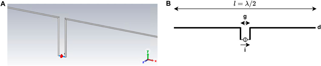
FIGURE 4. Electric dipole: (A) CST verification model, (B) schematic view of the ideal dipole.

FIGURE 5

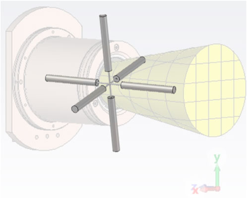
FIGURE 5. Use of a Hertzian dipole structure for electromagnetic representation of the thruster model‘s emission (schematic view).

Here, Z₀ = 120π Ω is the characteristic impedance in the far field, and c₀ ≈ 300 ⋅ 10⁶ m/s is the speed of light in vacuum. The composition of the fields will be discussed in order to understand this relationship. In the near field, field strengths exist depending on the angle θ and ϕ, as well as the radial component r (spherical coordinates). In the far field, the radial component is neglected because there is nearly a plane wave, and therefore, the electric field depends on θ. This becomes clear in Figure 6. The shape is created as the field lines exit at one end of the dipole and enter at the other.

FIGURE 6

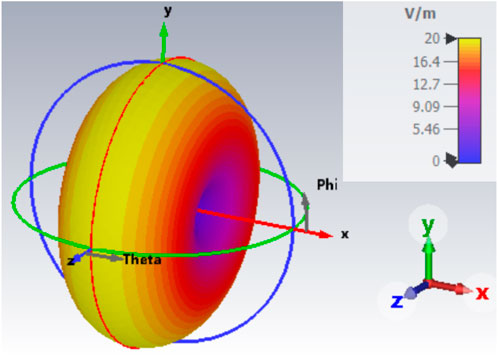
FIGURE 6. 3D electric far-field emissions of a Hertzian dipole in r =3 m distance and l = λ/2 (resonance). Dipole orientation in the x-direction.

The approximation in Eq. 8 assumes the most ideal boundary conditions, which can only be produced to a limited extent in CST. It is valid just in the far-field range and for short antenna structures (Gustrau, 2015), as in Eq. 9:

$l\ll \frac{\lambda }{10}=\frac{c_0}{10\cdot f}.(9)$

Here, λ is the wavelength. The verification environment, including all settings, is the same as that of the thruster model. The dipole’s assigned material is a perfect electric conductor, since Eq. 8 also assumes an optimal structure. The excitation is a current source with 1 A. The ideal Hertzian dipole structure has a total length of l = λ/2 in order to reach maximum radiation. This length is possible despite the condition from Eq. 9 because a real dipole can be concatenated from several ideal Hertzian dipoles. To validate the verification model, a comparison of the thus far ideal (theoretical) and a replicated dipole is necessary. To do this, the mechanical length of the replicated dipole must be adjusted because of the finite thickness d of the wire as well as the spatial environment. This correction is achieved with the multiplication factor A, which depends on the ratio of the wavelength to the cable diameter d respective to gap g of the dipole (Figure 5). The ratio of wavelength to diameter in the verification is λ/d = 1,000, while for the gap applies a ratio of g = λ/200 = 0.05 ⋅ λ. This results in a multiplication factor of A ≈ 0.95 according to Fig. 11.18 in Kark (2016). The mechanical length of the dipole as the verification model is calculated according to Eq. 10:

$l_{\text{m}}=A\cdot l=A\cdot \frac{\lambda }{2}.(10)$

The distance of the far-field measurements is r = 3 m. The consideration happens at l ≪ r since the far-field conditions are fulfilled here. Furthermore, the observation takes place in the resonance case, where the maximum phase position is analyzed. To use Eq. 8 for this verification case, a derivation is necessary: in the resonance case, the current coverage on the ideal dipole is exactly one sine half-wave (Jackson, 1998) (Figure 7). Thus, the current on the dipole depends on the ongoing position according to Eq. 11:

$i\left(x\right)=\widehat{i}\cdot \cos \left(k\cdot x\right),(11)$

FIGURE 7

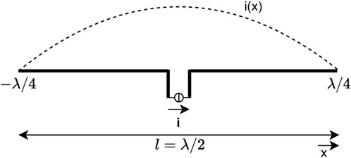
FIGURE 7. Current coverage of a Hertzian dipole at resonance. Dipole orientation in the x-direction.

where k is the wave number and can be calculated via $\frac{2\pi }{\lambda }$. This current behavior inserted at Eq. 8 results in Eq. 12:

$E_{\text{max}}\left(r\right)\approx \frac{Z_0}{2\cdot \lambda \cdot r}\cdot \int i\left(x\right)\mathrm{d}x=\frac{Z_0\cdot \widehat{i}}{\lambda \cdot r}\cdot {\int }_0^{\lambda /4}\cos \left(k\cdot x\right)\mathrm{d}x.(12)$

The supply current $\widehat{i}$ is taken as constant and the current curve as symmetrical starting from the center point. This yields Eq. 13:

$E_{\text{max}}\left(r\right)\approx \frac{Z_0\cdot \widehat{i}}{2\cdot \pi \cdot r},(13)$

with r = 3 m and $\widehat{i}=1\mathrm{A}$ following a maximum field strength of 20 V/m. As can be seen, it is frequency-independent since the equation is valid for the resonance case with l = λ/2. The results of the verification can be seen in Figure 8A. In a range from 100 MHz to 1 GHz 10, operating points are shown as proof. The electric far fields are given by calculation and verification. Here, a good agreement with deviations of less than 0.9% is shown (Figure 8B). The maximum deviation of 0.9% is taken as the error limit for the results in the next chapter. The higher the frequency, the better the match since CST calculates to a distance of r = 3 m. The consideration l ≪ r therefore becomes better.

FIGURE 8

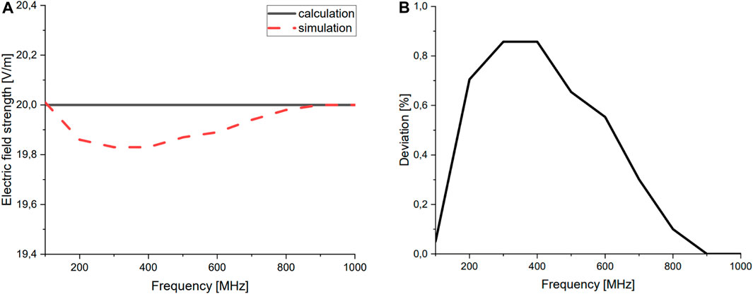
FIGURE 8. (A) Electric field strengths in V/m calculated on the basis of a Hertzian dipole in r =3 m distance, (B) % deviation between verification and calculation.

The remaining deviations can be described as follows: The derivation assumes perfect verification models and is implemented in the verification where possible. For example, a gap exists between both dipole ends, and the wires have a finitely small radius. Furthermore, the most ideal boundary conditions are assumed, where, in the verification, limits are reached due to computationally intensive processes. In addition, in the verification, the source itself is already radiating, which is unavoidable. Due to these explainable limitations and effects, the verification represents a good match with the calculation. Based on this good agreement, the verification model, including schematic and especially the simulation environment, is trusted.

6 Results

The results of the simulation are presented as follows. To identify possible ion beam configurations and their impact on the electric far field, several simulations were performed, and one parameter was changed in each case (Table 1). The RIT is briefly explained to better understand the simulation parameters. Generally, the RFG provides energy to the thruster coil; it thus controls the operating point of the thruster, which makes it a crucial part of the RIT assembly. A RIT consists of a coil wound around a vessel, where a plasma is generated. With a grid structure at this vessel to the outside, the ions will be accelerated and extracted to generate thrust. There is an electric field between the grids because a high voltage is connected from the outside. The RFG is operated at different voltages of the full bridge as well as frequencies, depending on the operating points. For the ion beam, the parameters’ divergence angle, beam current, and grid voltage are changed. The last two parameters contribute directly to the conductivity (Eqs. 4, 5). For all simulations, the distance of the far-field measurement is 3 m.

TABLE 1

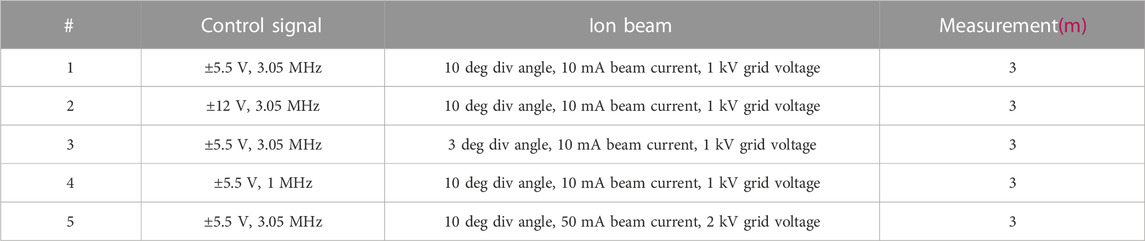
TABLE 1. Simulation characteristics.

First, the simulation with and without the ion beam is investigated. This determines the general importance of the research. Without a decisive difference, further investigation of the ion beam would not be important as no significant degradation on the EMC has occurred.

The emissions in the far field are shown in Figure 9 for simulation #5 with and without the ion beam at different frequencies. It is qualitatively evident that the ion beam has a considerable influence on the overall emission characteristics of strength and shape, increasing the emission values and the relevant radiation range. A diagram with concrete electric field strengths is shown in Figure 10A, where the ion beam provides a significant increase in electric field strength in the far field. This increase is explained, on the one hand, by the newly established antenna effect due to the conductive ion beam. In addition, the ion beam conducts more effective emissions out of the thruster housing because it is directly connected to the plasma inside. The emissions in the high-frequency range are generated by the feed signal of the full bridge of the RFG. It is a square wave signal, which contains high-frequency components due to the sharp rising and falling edges.

FIGURE 9

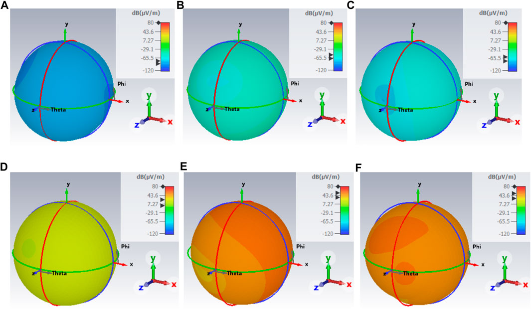
FIGURE 9. 3D electric far field in 3 m distance for simulation #5: (A) without ion beam at f =101 MHz, (B) without ion beam at f =505 MHz, (C) without ion beam at f =1 GHz, (D) with ion beam at f =101 MHz, (E) with ion beam at f =505 MHz, and (F) with ion beam at f =1 GHz.

FIGURE 10

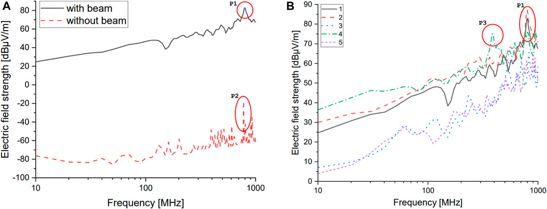
FIGURE 10. Electric far field in 3 m distance: (A) simulation #1 with and without ion beam; (B) all simulation variants.

We now consider the individual changes of the ion beam properties. Figure 10B shows all five configurations; the legend numbers refer to those in Table 1. In general, it can be seen that the progressions of the emission curves are the same: there are isolated spikes at different frequencies, and the level of emissions varies, which will be discussed in more detail below: A higher voltage of the RFG output, and thus a higher power input to the thruster coil, ensures higher emissions. At frequencies above 500 MHz, the electric field strength is similar. At a voltage of 5.5 V, an amplitude of 1.3 A is achieved; at 12 V, it is 2.8 A. A smaller divergence angle has a positive effect on the emission characteristics of the thruster. In the lower frequency range, a reduction from 10° to 3° provides an emission optimization of up to 20 dB, which corresponds to a factor of 10. As the frequency increases, this gap becomes smaller and is reduced to about 10 dB (factor of 3). When the frequency of the drive signal is reduced from 3.05 MHz to 1 MHz, the field strength is increased in the lower frequency range up to 300 MHz. In the further course, the emissions of both frequencies almost coincide. In simulation #5, the ion beam has a higher conductivity, which causes the emissions to drop sharply. The graph is comparable to that from simulation #3. The same deviations from the reference from simulation #1 are achieved.

To further characterize the results, significant resonance locations are now discussed. Resonances P1 and P2 (Figure 10A) are due to the thruster geometry—more specifically, the extraction grids. Previous research shows that resonances in this high-frequency range are roughly proportional to the size of the extraction grid (Baruth, 2017). The simulation confirms this as resonance also occurs with and without the ion beam. The resonance P3 (Figure 10B) is shifted due to the changed frequency of the drive signal (simulation characteristic #3) but can still be assigned to the grid geometry.

In summary, more injected power and a larger divergence angle of the beam mean higher emissions. If the conductivity of the beam is increased or if the divergence angle is decreased, the emission of the thruster assembly is reduced. The parameters of the ion beam provide the characteristics of the radiation. To generate low radiation, it is necessary to adjust these parameters depending on the possibilities. Varying the frequency of the excitation signal makes a difference, but it is not as crucial as changing the direct parameters of the ion beam.

7 Discussion

The simulation was thus successfully established. The RIT-4 model was supplemented with the ion beam replica and examined. The ion beam has a high influence on the emission characteristics of the thruster assembly. Likewise, the properties of the ion beam play a major role; depending on the design, more or fewer emissions can be expected and quantitatively predicted with acceptable accuracy. These studies contribute to the expansion of science because new insights are gained into the emission characteristics of the thruster. Furthermore, by entering the thruster parameters as well as the operating point, it is possible to discover the emissions of the thruster and ion beam combination.

The next steps are to embed this knowledge into the overall system. Elaborations exist on the RFG, the thruster itself, and the corresponding cabling. The insertion of a neutralizer with electron emission is planned for future research. These results will be combined to lead to a holistic EMC system. Further measurements need to be made with the EMC vacuum chamber that include comparable setups. If these two procedures match, a good prediction can be made with the help of the simulation, which provides information about EMC behavior even before the development of the thruster assembly. This results in shorter test times and less post-development. Furthermore, other EMC areas such as near-field can be analyzed in future research. Moreover, the possibility of extending the model to other ion thrusters, such as a Hall effect thruster, and predicting their ion thruster behavior should be explored.

Data availability statement

The raw data supporting the conclusion of this article will be made available by the authors without undue reservation.

Author contributions

YR: conceptualization, data curation, formal analysis, investigation, methodology, resources, software, validation, visualization, writing–original draft, and writing–review and editing. RT: writing–review and editing, and methodology. UP: funding acquisition, project administration, and writing–review and editing. CV: methodology, project administration, supervision, validation, and writing–review and editing.

Funding

The authors declare that financial support was received for the research, authorship, and/or publication of this article. This work was financially supported by the German Federal Ministry of Education and Research, grant number 13FH173PX8.

Acknowledgments

This publication represents a component of the corresponding author’s doctoral thesis in the Department of Physics at the Justus-Liebig-University Giessen, Germany, in cooperation with Technische Hochschule Mittelhessen—University of Applied Sciences at the Graduate Centre of Engineering Sciences at the Research Campus of Central Hessen.

Conflict of interest

The authors declare that the research was conducted in the absence of any commercial or financial relationships that could be construed as a potential conflict of interest.

Publisher’s note

All claims expressed in this article are solely those of the authors and do not necessarily represent those of their affiliated organizations, or those of the publisher, the editors, and the reviewers. Any product that may be evaluated in this article, or claim that may be made by its manufacturer, is not guaranteed or endorsed by the publisher.

References

Baruth, T. (2017). Analysis on the electromagnetic compatibility of radio-frequency ion thrusters using a RIT4. Giessen, Germany: University of Giessen. Available at: http://geb.uni-giessen.de/geb/volltexte/2017/12495/.

Google Scholar

Becker, R., and Herrmannsfeldt, W. B. (1992). i g u n−A program for the simulation of positive ion extraction including magnetic fields. Rev. Sci. Instrum. 63, 2756–2758. doi:10.1063/1.1142795

CrossRef Full Text | Google Scholar

Chabert, P., and Braithwaite, N. (2011). Physics of radio-frequency plasmas. 1. Cambridge: Cambridge University Press. ISBN 978–0–521–76300–4.

Google Scholar

Dobkevicius, M., and Feili, D. (2016). A coupled performance and thermal model for radio-frequency gridded ion thrusters. Eur. Phys. J. D. 70, 227. doi:10.1140/epjd/e2016-70273-7

CrossRef Full Text | Google Scholar

European cooperation for space standardization (2012). ECSS-E-ST-20-07C rev. 1. Noordwijk (Netherlands): ESA-ESTEC Requirements and Standards Division.

Google Scholar

Goebel, D. M., and Katz, I. (2008). Fundamentals of electric propulsion: ion and Hall thrusters. New Jersey, United States: Wiley. ISBN 978-0-470-42927-3.

Google Scholar

Gustrau, F. (2015). Elektromagnetische verträglichkeit. Munich, Germany: Hanser. ISBN 978-3-446-44301-3.

Google Scholar

Holste, K., Dietz, P., Scharmann, S., Keil, K., Henning, T., Zschätzsch, D., et al. (2020). Ion thrusters for electric propulsion: scientific issues developing a niche technology into a game changer. Rev. Sci. Instrum. 91, 061101. doi:10.1063/5.0010134

PubMed Abstract | CrossRef Full Text | Google Scholar

International Electrotechnical Commission (2018). IEC standard 60050-161-01-07: international electrotechnical vocabulary: electromagnetic compatibility: basic concepts.

Google Scholar

Jackson, J. D. (1998). Classical electrodynamics. 3. New Jersey, United States: Wiley. ISBN 978-0-471-30932-1.

Google Scholar

Kalvas, T., Tarvainen, O., Ropponen, T., Steczkiewicz, O., Ärje, J., and Clark, H. (2010). IBSIMU: a three-dimensional simulation software for charged particle optics. Rev. Sci. Instrum. 81, 02B703. doi:10.1063/1.3258608

PubMed Abstract | CrossRef Full Text | Google Scholar

Kark, K. W. (2016). Antennen und Strahlungsfelder. 6. Cham: Springer Vieweg. ISBN 978-3-658-13965-0 (eBook).

Google Scholar

Reeh, A., Probst, U., and Klar, P. J. (2017). “3D ion extraction code incorporated self-consistently into a numerical model of a radio-frequency ion thruster,” in 35th International Electric Propulsion Conference, Daniłko, Dariusz, October 8 – 12, 2017. Atlanta, Georgia (US), IEPC-2017-326.

Google Scholar

Reeh, A., Probst, U., and Klar, P. J. (2019). Global model of a radio-frequency ion thruster based on a holistic treatment of electron and ion density profiles. Eur. Phys. J. D. 73, 232. doi:10.1140/epjd/e2019-100002-3

CrossRef Full Text | Google Scholar

Reynolds, T. W. (1971). Mathematical representation of current density profiles from ion thrusters. Cleveland, Ohio: NASA Lewis Research Center. Technical Report NASA TN-D6334.

Google Scholar

Rover, Y., Thüringer, R., Volkmar, C., Probst, U., Kiefer, F., Holste, K., et al. (2023). Semi-anechoic chamber for electromagnetic compatibility tests of electric propulsion thrusters. J. Electr. Propuls. 2, 3. doi:10.1007/s44205-023-00039-w

CrossRef Full Text | Google Scholar

Rover, Y., and Volkmar, C. (2022). “Verification of a radio-frequency generator model in a full-wave 3D EM simulation,” in IEEE aerospace conference (Montana (US): Big Sky). 978-1-6654-3760-8/22/$31.00.

CrossRef Full Text | Google Scholar

Scholze, F., Bundesmann, C., Eichhorn, C., and Spemann, D. (2019). “Determination of the beam divergence of a gridded ion thruster using the AEPD platform,” in 36th International Electric Propulsion Conference, Vienna, Austria, September 15-20, 2019. IEPC-2019-A-738.

Google Scholar

Symeonidis, S. (2018). CST-MATLAB-API. v1.0.0. doi:10.5281/zenodo.1237969

CrossRef Full Text | Google Scholar

Zhang, H., Zhang, Y., Huang, C., Yuan, Y., and Cheng, L. (2021). Spacecraft electromagnetic compatibilities Technologies. Cham: Springer. ISBN 978-981-15-4781-2. doi:10.1007/978-981-15-4782-9

CrossRef Full Text | Google Scholar