A comparative analysis of reinforcement learning algorithms for earth-observing satellite scheduling

Deep reinforcement learning (DRL) has shown promise for spacecraft planning and scheduling due to the lack of constraints on model representation, the ability of trained policies to achieve optimal performance with respect to a reward function, and fast execution times of the policies after training. Past work investigates various problem formulations, algorithms, and safety methodologies, but a comprehensive comparison between different DRL methods and problem formulations has not been performed for spacecraft scheduling problems. This work formulates two Earth-observing satellite (EOS) scheduling problems with resource constraints regarding power, reaction wheel speeds, and on-board data storage. The environments provide both simple and complex scheduling challenges for benchmarking DRL performance. Policy gradient and value-based reinforcement learning algorithms are trained for each environment and are compared on the basis of performance, performance variance between different seeds, and wall clock time. Advantage actor-critic (A2C), deep Q-networks (DQN), proximal policy optimization (PPO), shielded proximal policy optimization (SPPO) and a Monte Carlo tree search based training-pipeline (MCTS-Train) are applied to each EOS scheduling problem. Hyperparameter tuning is performed for each method, and the best performing hyperparameters are selected for comparison. Each DRL algorithm is also compared to a genetic algorithm, which provides a point of comparison outside the field of DRL. PPO and SPPO are shown to be the most stable algorithms, converging quickly to high-performing policies between different experiments. A2C and DQN are typically able to produce high-performing policies, but with relatively high variance across the selected hyperparameters. MCTS-Train is capable of producing high-performing policies for most problems, but struggles when long planning horizons are utilized. The results of this work provide a basis for selecting reinforcement learning algorithms for spacecraft planning and scheduling problems. The algorithms and environments used in this work are provided in a Python package called bsk_rl to facilitate future research in this area.

1 Introduction

The need for spacecraft autonomy is growing as missions become more ambitious and the number of space-based assets grows, which places a burden on spacecraft operators and increases operational costs. In particular, autonomous on-board planning and scheduling capabilities offer promise due to their ability to plan in a closed-loop fashion, responding to off-nominal conditions or opportunistic science events without intervention from the ground. The first example of such a system is the Remote Agent, which was used on board NASA’s Deep Space One spacecraft to demonstrate goal-based commanding, on-board planning, robust execution, and fault protection (Bernard et al., 1998; Muscettola et al., 1998; Bernard et al., 1999). The Automated Scheduling/Planning Environment (ASPEN) is a ground-based tool used for a number of missions that can autonomously generate a plan (Fukunaga et al., 1997). The Continuous Activity Scheduling Planning Execution and Replanning (CASPER) tool can be used in conjunction with ASPEN to modify and repair these plans on board real spacecraft (Knight et al., 2001). ASPEN and CASPER have been utilized in the Earth-Observing 1 (Chien et al., 2005; Chien et al., 2019; Chien et al., 2020) and IPEX (Chien et al., 2016) missions for autonomous planing and replanning, increasing science return and reducing operational costs. The success of these tools demonstrates the need for on-board planning and scheduling capabilities.

Reinforcement learning has emerged as a potential method for increasing autonomy in a variety of spacecraft decision-making domains, such as guidance, navigation, and control (GNC) and planning and scheduling due to its inherent closed-loop planning nature. The objective of reinforcement learning is to learn a policy that maps states to actions to maximize a numerical reward function (Sutton and Barto, 2018). The policy may be represented in tabular form or with a neural network, which can be executed on-board in milliseconds. References (Blacker et al., 2019; Dunkel et al., 2022) demonstrate the execution of neural networks on flight processors (or processors currently undergoing validation for flight), ranging from milliseconds to seconds of execution time. Due to fast execution times, a low memory footprint, and the potential for optimal policies with respect to the reward function, reinforcement learning is an excellent candidate for both low- and high-level spacecraft autonomy.

Reinforcement learning has been used for planetary landing (Gaudet et al., 2020a; Gaudet et al., 2020b; Furfaro et al., 2020; Scorsoglio et al., 2022), small body proximity operations (Gaudet et al., 2020c; Gaudet et al., 2020d; Federici et al., 2022a; Takahashi and Scheeres, 2022), and spacecraft rendezvous, proximity operations, and docking (RPOD) (Fed et al., 2021; Hovell and Ulrich, 2021; Oe et al., 2021; Federici et al., 2022b; Hovell and Ulrich, 2022; Dunlap et al., 2023). Proximal policy optimization (PPO), a policy-based deep reinforcement learning algorithm, is the most popular reinforcement learning algorithm in the surveyed works, likely due to its stable convergence properties and ease of implementation. To handle partial observability (e.g., thruster failures), many of the cited works utilize a recurrent policy version of PPO, which uses a recurrent neural network in the policy to learn from a sequence of observations as opposed to a single observation or a stack of observations. In addition to partial observability, treatment of safety constraints is a constant challenge when using reinforcement learning for spacecraft decision-making problems. The simplest and most popular approach is to add the safety constraints to the reward function in the form of a failure penalty. However, constraint violation penalties in the reward function does not mean they will not be violated. Dunlap et al. address system safety with run time assurance (RTA) integrated into training in Dunlap et al. (2023), which guarantees the policy will not take unsafe actions.

In addition to solving GNC problems, reinforcement learning has been applied to many Earth-observing satellite (EOS) scheduling problems. However, each paper solves a different problem using a different algorithm, such as asynchronous advantage actor-critic (A3C) (Haijiao et al., 2019), REINFORCE (Zhao et al., 2020), and deep Q-networks (DQN) (He et al., 2020). Furthermore, these works often insufficiently model resources such as battery charge, data storage availability, and reaction wheel speeds, as well as their impact on the EOS scheduling problem. Harris et al. demonstrate utilizing shielded PPO (SPPO) for EOS scheduling with battery and reaction wheel speed constraints. SPPO bounds the decision-making agent’s actions during training and deployment such that only safe actions are taken (Harris et al., 2021). Shielded deep reinforcement learning utilizes a linear temporal logic specification to monitor the actions output by the policy, overriding the actions if they violate the LTL specification (Alshiekh et al., 2018). Herrmann and Schaub utilize a similar technique, using an extension of the safety shield developed by Harris and Schaub as a rollout policy inside of Monte Carlo tree search (MCTS) (Herrmann and Schaub, 2021; Herrmann and Schaub, 2023a) for EOS scheduling problems that include battery, reaction wheel speeds, and on-board data resource constraints. MCTS is used to generate training data, which is regressed over using artificial neural networks to produce a generalized state-action value function, which may be executed on-board the spacecraft in seconds. This training pipeline is referred to as MCTS-Train. Eddy and Kochenderfer also apply MCTS to a semi-Markov Decision Process (SMDP) formulation of the EOS scheduling problem with resource constraints regarding power and data storage, demonstrating near-optimal performance compared to a mixed integer programming formulation and solution (Eddy and Kochenderfer, 2020). While each of the aforementioned works provide novel contributions to the field of EOS scheduling, they do not compare reinforcement learning algorithms to one another in a comprehensive way. In addition to these gaps in the literature, the relationship between the different RL algorithms, their hyperparameters, and performance variance between different initial seeds is not well documented.

To address these issues, this work provides a comprehensive comparison, complete with hyperparameter searches, between various reinforcement learning algorithms for two EOS scheduling problems. Of interest is how efficient and robust five DRL methods are in training a neural network to do autonomous on-board spacecraft scheduling. The neural networks are tested for a simple and complex benchmark spacecraft environments to assess their performance, robustness, and training time. The paper is organized as follows. First, each EOS scheduling problem is described: a multi-sensor EOS scheduling problem and an agile EOS scheduling problem. The simulation architecture and Markov decision process formulation of each problem is described. Then, the methods used to solve each problem are presented. This work implements Proximal policy optimization, shielded proximal policy optimization, advantage actor-critic (A2C), MCTS-Train, and deep Q-networks to solve each scheduling problem. Hyperparameter searches are shown for each algorithm, and each algorithm is compared on the basis of performance across various hyperparameters, performance variance between training seeds, and wall clock time. Each algorithm is also compared to a genetic algorithm, a common algorithm used for comparisons in work using RL for EOS scheduling due to the ease of using the simulator and reward function as the evaluation function.

2 Problem statement

In the Earth-observing satellite scheduling problem, one or more satellites attempt to maximize the amount of science data collected over some planning horizon. Depending on the problem formulation, data downlink and resource constraints may also be considered. Furthermore, several science objectives such as agile imaging, area coverage, etc., may be considered. For this comparison work, two versions of the Earth-observing satellite scheduling problem are considered. The first EOS scheduling problem, the multi-sensor EOS scheduling problem, is meant to be the simpler of the two environments as the satellite only needs to collect images (not downlink) to get positive reward and only needs to manage two resources: battery and reaction wheel speeds. The second EOS scheduling problem, the agile EOS scheduling problem, is meant to be more challenging as the satellite must manage battery, reaction wheel speeds, and data storage. Furthermore, the satellite has individual imaging targets available to it that it must collect and then downlink to receive reward.

For each problem, a satellite in low Earth orbit images ground targets while managing power and reaction wheel speed constraints. Power is generated by the solar panels and stored within a battery. Power is consumed by instruments, transmitters, and reaction wheels. The reaction wheels are used to control the attitude of the spacecraft as attitude references are switched between during mode switching, and momentum is built up within the reaction wheels using a disturbance torque. The satellites perform their science objectives and manage their resources by entering into various operational modes such as imaging, downlink, charging, and desaturation. Concept figures for each problem are provided in Figure 1. The details regarding the agile EOS and multi-sensor EOS MDP formulations are provided in References 33 and 35, respectively. Furthermore, the simulators used for each problem may be found on the develop branch of the bsk_rl Python library¹. However, a summary regarding each Markov decision process will be provided here for reference.

FIGURE 1

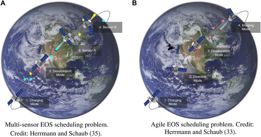
FIGURE 1. Earth-observing satellite scheduling problems. (A): Multi-sensor EOS scheduling problem. Reproduced with permission from Herrmann and Schaub (Herrmann and Schaub, 2023b). (B): Agile EOS scheduling problem. Reproduced with permission from Herrmann and Schaub (Herrmann and Schaub, 2023a).

Each EOS scheduling problem is formulated as a Markov decision process (MDP). An MDP is a decision-making problem in which an agent takes an action a_i in a state s_i following some policy, $\pi :\mathcal{S}\to \mathcal{A}$, which is a mapping from states to actions. The objective is to solve for the policy that maximizes a numerical reward function, R (s_i, a_i). The reward function is used to encode the desired outcomes of the decision-making agent, i.e., what tasks it should perform and what areas of the state it should enter into or avoid. The decision-making agent receives a reward at each step based on this reward function, r_i = R (s_i, a_i). Following each action, the decision-making agent transitions to a new state following some transition function. MDPs adhere to what is known as the Markov assumption, which states that the next state is conditionally dependent only on the current state and action. Explicit representations of the transition function are often represented with a conditional probability distribution, T (s_i+1|s_i, a_i). However, real world problems are often difficult to cast as conditional probability distributions. Generative transition functions that utilize the known dynamics of the system or sample from complicated underlying distributions are often more appropriate. These are represented with s_i+1, r_i ∼ G (s_i, a_i).

2.1 Multi-sensor EOS scheduling problem

In the multi-sensor EOS scheduling problem, a nadir-pointing satellite attempts to maximize the sum of imaging targets collected with one of two sensor types, A or B, while managing power and reaction wheel speeds. The set of all imaging targets is referred to as T. The satellite only ever considers the next upcoming target. The planning horizon, which is the total length of time considered for planning and scheduling, is broken into a number of equal length decision-making intervals. This set of intervals is referred to as I. This work explores two separate planning horizon lengths: 45 and 90 decision-making intervals, which has a large impact on the problem complexity. Each decision-making interval lasts for 3 minutes.

2.1.1 State space

Selecting the state space for any realistic decision-making problem is a challenging endeavor. The state space must contain all information relevant to the decision-making problem that ensures the Markov assumption is satisfied. For the EOS scheduling problem, this is difficult to completely satisfy due to the complexity of the problem, which requires a massive state space to fully capture. Therefore, the state space is selected to contain the information that is most relevant to the decision-making problem.

The state space for the multi-sensor EOS scheduling problem is defined as:

$\mathcal{S}={\mathcal{S}}_{\text{sat}}\times {\mathcal{S}}_{\text{targets}},(1)$

where state space of the satellite is defined as:

${\mathcal{S}}_{\text{sat}}={\mathcal{S}}_{\text{pos}}\times {\mathcal{S}}_{\text{vel}}\times {\mathcal{S}}_{\text{att}}\times {\mathcal{S}}_{\text{wheels}}\times {\mathcal{S}}_{\text{power}}\times {\mathcal{S}}_{\text{eclipse}}.(2)$

The state returned to the decision-making agent at decision interval i is defined as s_i ∈ S:

$s_i=\left({}^{\text{SEZ}}\mathbf{r},{}^{\text{SEZ}}\mathbf{v},\Vert {\mathit{\sigma }}_{\mathcal{B}/\mathcal{R}}\Vert ,{\Vert }^{\mathcal{B}}{\mathit{\omega }}_{\mathcal{B}/\mathcal{N}}\Vert ,\Vert \mathbf{\Omega }\Vert ,\text{battery},\text{access},\text{sensor},\text{eclipse}\right).(3)$

The position and velocity, ^SEZr and ^SEZv, of the satellite are expressed in the topocentric horizon coordinate system, or SEZ frame. This coordinate system is defined relative to the imaging target and is selected to ensure the policy is target agnostic. Attitude information is provided in the form of spacecraft attitude, angular velocity, and reaction wheel speeds. The attitude of the satellite is provided as the magnitude of the modified Rodriguez parameters (MRP), (Schaub and Junkins, 2018), ${\mathit{\sigma }}_{\mathcal{B}/\mathcal{R}}$, which is the rotation from the reference frame to the body frame. The magnitude of the angular velocity of the satellite,${}^{\mathcal{B}}{\mathit{\omega }}_{\mathcal{B}/\mathcal{N}}$, is provided in the body frame. The magnitude of the reaction wheel speeds is given by Ω. Several states are also included for the purposes of power management. The percent charge of the battery is provided using the battery variable, and the eclipse variable is a binary variable that indicates whether the satellite is in eclipse. The last few states deal with target access and which type of sensor the target shall be imaged with to receive reward. The access variable is a binary variable that indicates whether the satellite has access to the next upcoming imaging target, and the sensor variable is a binary variable that indicates which type of sensor the satellite shall image the upcoming target with.

2.1.2 Action space

Like the state space, the action space is designed to fulfill the science objectives and manage the resource constraints. Each action represents a distinct spacecraft mode. Descriptions of each are provided below.

1. Charge

• The satellite turns off its imager and transmitter and points its solar panels at the Sun to charge the battery.

2. Desaturate

• The satellite turns off its imager and transmitter and points its solar panels at the Sun. Reaction wheel momentum is mapped to thrust commands, which are executed to remove momentum from the wheels.

3. Image with sensor A

• The satellite turns on imager A, and points it in the nadir direction. An image is taken when requirements are met.

4. Image with sensor B

• The satellite turns on imager B, and points it in the nadir direction. An image is taken when requirements are met.

In the imaging mode, the satellite uses an MRP feedback control law and its reaction wheels to point the instrument in the nadir direction and collect an image of the target when the satellite meets the elevation requirement of 60°. Unlike the agile EOS scheduling problem, the spacecraft does not point its instrument directly at the ground target in the multi-sensor EOS scheduling problem. However, the spacecraft must use the correct sensor type to collect an image.

2.1.3 Reward function

A piecewise reward function is developed to mathematically formalize the objectives of the multi-sensor EOS scheduling problem. The first condition checked for is failure. Failure is true only if the reaction wheels exceed their maximum speed or if the batteries are empty. If failure does not occur, the imaging mode is checked next. If the satellite images the next upcoming target with the correct sensor type, a small reward bonus is returned. This reward bonus is equal to one 1 divided by the product of the total number of targets (50 for the multi-sensor EOS problem) and the summation of 1 and the square of the attitude error. The component due to imaging has a maximum reward of 1, which assumes the satellite images every target with the correct sensor type and zero attitude error.

$R\left(s_i,a_i,s_{i+1}\right)=\left\{\begin{array}{cc}-1\hfill & \text{if\hspace{0.17em}failure}\hfill \\ \frac{1}{|T|\left(1+{ϵ}_{\text{att}}^2\right)}\hfill & \text{if}e{l}_{\text{sc}}>e{l}_{\text{min}}\text{and}{a}_i\text{\hspace{0.17em}is\hspace{0.17em}preferred}\hfill \\ 0\hfill & \text{\hspace{0.17em}otherwise}\hfill \end{array}\right.(4)$

2.1.4 Gymnasium environment

The generative transition function s_i+1, r_i ∼ G (s_i, a_i) is modeled using a high-fidelity astrodynamics simulation framework, Basilisk² (Kenneally et al., 2020). Basilisk implements simulation and flight software code in C/C++, but provides a Python interface for scripting. The Basilisk simulation is wrapped within a Gymnasium³ environment, which provides a standard interface that allows reinforcement learning libraries to interact with the simulation. The agent passes actions to the Gymnasium environment, which turns certain Basilisk modules on or off. The simulation is integrated forwards in time for 6 minutes at a 1-s integration time step. The environment constructs the observation and reward, which is returned to the decision-making agent. This process is demonstrated in Figure 2. For the multi-sensor EOS scheduling problem, Basilisk simulates a satellite in low Earth orbit complete with an attitude control system and power system.

FIGURE 2

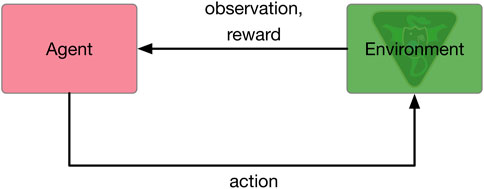
FIGURE 2. Agent-environment interface.

Depending on the action taken, a new reference frame for attitude pointing is set. The attitude control system utilizes a modified Rodriguez parameter (MRP) feedback control law for pointing, sending torque commands to the reaction wheels, which align the spacecraft attitude with the desired reference. This feedback control law is active regardless of the satellite mode taken, but the attitude reference changes. Desaturation is performed by mapping the wheel momentum to thruster on-time commands.

A power system is also modeled in Basilisk. A battery is used to store the power generated by solar panels, which generate power based on the efficiency of the panels and incidence angle of the Sun. Several power sinks are also modeled, such as the instruments and the reaction wheels. These all consume power stored within the battery.

2.2 Agile EOS scheduling problem

In the agile EOS scheduling problem, a satellite with three-axis attitude control capabilities attempts to image ground targets with a single imaging sensor and downlink them to ground stations located on the surface of the Earth. The set of all imaging targets is referred to as T, and a subset of T that contains the next J upcoming, unimaged targets is referred to as U. Each target within U is referred to as c_j. This set is defined with Eq. 5, where D is the set of imaged or passed targets.

$U=\left\{c_j\in \left(T-D\right)|\forall j\in \left[0,J\right)\right\}(5)$

At each decision-making interval, the satellite only considers the targets in the subset U for imaging. This is done to reduce the size of the action space to some number of upcoming targets that are available for imaging, not the entire global set T. For this work, |U| = J = 3 and |T| = 135. Past work has shown that increasing the size of U past three targets only results in marginal performance improvements for this target density (Herrmann and Schaub, 2023a).

The satellite has a data buffer in which the collected images are stored. The data buffer has a maximum capacity, and the satellite must downlink the collected images to various ground stations on the surface of the Earth to avoid overfilling the data buffer. The satellite has a power system with a battery, solar panels, and various power sinks such as the imager, transmitter, and reaction wheels. The reaction wheels have a maximum speed constraint, and thrusters on board the satellite are used to remove momentum from the thrusters.

2.2.1 State space

The state space for the multi-sensor EOS scheduling problem is defined as:

$\mathcal{S}={\mathcal{S}}_{\text{sat}}\times {\mathcal{S}}_{\text{ground\hspace{0.17em}stations}}\times {\mathcal{S}}_{\text{targets}},(6)$

where state space of the satellite is defined as:

${\mathcal{S}}_{\text{sat}}={\mathcal{S}}_{\text{pos}}\times {\mathcal{S}}_{\text{vel}}\times {\mathcal{S}}_{\text{att}}\times {\mathcal{S}}_{\text{wheels}}\times {\mathcal{S}}_{\text{power}}\times {\mathcal{S}}_{\text{buffer}}\times {\mathcal{S}}_{\text{eclipse}}.(7)$

The state returned to the decision-making agent at decision interval i is defined as s_i ∈ S:

$s_i=\left({}^{\mathcal{E}}\mathbf{r},{}^{\mathcal{E}}\mathbf{v},{}^{\mathcal{H}}{\mathbf{r}}_{\mathbf{1}},p_1,\cdots ,{}^{\mathcal{H}}{\mathbf{r}}_j,p_j,\Vert {\mathit{\sigma }}_{\mathcal{B}/\mathcal{R}}\Vert ,{\Vert }^{\mathcal{B}}{\mathit{\omega }}_{\mathcal{B}/\mathcal{N}}\Vert ,\mathbf{\Omega },\text{battery},\text{buffer},\text{downlinked},\text{eclipse})\right..(8)$

The Earth-centered, Earth-fixed reference frame is denoted with $\mathcal{E}$, the spacecraft Hill frame is denoted with $\mathcal{H}$, and the spacecraft body frame is denoted with $\mathcal{B}$. The position and velocity of the satellite provide the geometric information relevant to the access to the ground stations, which are fixed in the ECEF frame. The position of the ground targets in the Hill frame, ${}^{\mathcal{H}}{\mathbf{r}}_j$, and their associated priorities, p_j, provide the necessary information regarding the upcoming targets. The attitude of the satellite is represented with ${\mathit{\sigma }}_{\mathcal{B}/\mathcal{R}}$, and the angular velocity of the satellite is represented with ${}^{\mathcal{B}}{\mathit{\omega }}_{\mathcal{B}/\mathcal{N}}$. The reaction wheel speeds are represented with Ω. The battery state, data buffer state, and downlinked state are represented with the variables battery, buffer, and downlinked, respectively. The battery and buffer variables are the percent fill of each resource. The downlinked state represents how much data was downlinked over the last decision-making interval. The eclipse state is represented with the binary eclipse variable, which is 1 if the satellite is in eclipse and 0 otherwise. Note that each state is feature engineered such that they are approximately in the range of [-1, 1]. This is done to improve the learning performance of the agent.

2.2.2 Action space

Like the state, the actions are designed to fulfill the science objectives and manage the resource constraints. Each action represents a distinct spacecraft mode. Descriptions of each are provided below.

1. Charge

• The satellite turns off its imager and transmitter and points its solar panels at the Sun to charge the battery.

2. Desaturate

• The satellite turns off its imager and transmitter and points its solar panels at the Sun. Reaction wheel momentum is mapped to thrust commands, which are executed to remove momentum from the wheels.

3. Downlink

• The satellite turns off its imager and turns on the transmitter. Data is downlinked to ground stations as they come into view of the satellite.

4. Image target c₀ ∈ U

⋮

6. Image target c₂ ∈ U

• The satellite turns of its transmitter and turns on the imager. The satellite points the imager at the associated ground target and takes an image when requirements are met. The image is saved in the data buffer.

2.2.3 Reward function

A piecewise reward function is developed based on the objectives of the agile EOS scheduling problem. This reward function is provided in Eq. 9. The first condition checked for is failure, which is true if the satellite overfills the data buffer, exceeds the maximum reaction wheel speeds, or empties the battery. If a failure does not occur and a downlink mode is initiated, the ground targets in T are looped through to check if they were downlinked for the first time or not. Each target is checked using the downlinked indicator, d_j, input into the function in Eq. 10, which returns one over the target priority if the target was not downlinked at decision-making interval i and was downlinked at decision-making interval i + 1. For each target downlinked for the first time, one divided by the priority of the target and the number of decision-making intervals is returned. This component is formulated such that the maximum reward from downlink is 1. If failure is not true and the imaging mode is initiated, that target is checked to determine if it was imaged for the first time or not. If so, 0.1 divided by the target priority and number of decision-making intervals is returned. This component is formulated such that the total possible reward from imaging is 0.1. Finally, if none of these conditions are true, 0 reward is returned.

$R\left(s_i,a_i,s_{i+1}\right)=\left\{\begin{array}{cc}-1\hfill & \text{if\hspace{0.17em}failure}\hfill \\ \frac{1}{|I|}{\sum }_j^{|T|}H\left(d_j\right)\hfill & \text{if\hspace{0.17em}}\neg \text{failure\hspace{0.17em}}\wedge a_i\text{\hspace{0.17em}is\hspace{0.17em}downlink}\hfill \\ \frac{0.1}{|I|}H\left(w_j\right)\hfill & \text{if\hspace{0.17em}}\neg \text{failure\hspace{0.17em}}\wedge a_i\text{\hspace{0.17em}is\hspace{0.17em}image\hspace{0.17em}}{c}_j\hfill \\ 0\hfill & \text{\hspace{0.17em}otherwise}\hfill \end{array}\right.(9)$

$H\left(x_j\right)=\left(1/p_j\right)\text{if\hspace{0.17em}}\neg x_{j_i}\wedge x_{j_{i+1}}(10)$

2.2.4 Gymnasium environment

The generative transition function for the agile EOS scheduling problem is also modeled using a Basilisk Gymnasium environment. The simulator is more complicated than that of the multi-sensor EOS scheduling problem. An attitude control system, power system, and data storage system are modeled. The imager takes an image once the attitude reference is below the desired threshold and target access constraints are met. The attitude error threshold is ϵ_att = 0.1 rad and the target access elevation constraint is 45°. This image is stored in a simulated data buffer. The images contained within the data buffer are downlinked to simulated ground stations if the transmitter is active and access requirements are met (a minimum elevation of 10°). The physical ground station locations are modeled in Basilisk, and the access is computed according to the location of the spacecraft and ground station in question. Power sinks are added to the power system for the transmitter.

3 Methods

Deep reinforcement learning aims to solve reinforcement learning problems by learning a parameterized policy π_θ(a|s), a parameterized value function V_θ(s), or a parameterized state-action value function Q_θ(s, a) (Sutton and Barto, 2018). The policy is a probability distribution over actions conditioned on the state. The value function associated with a policy is the expected return from a given state following that policy. The optimal value function, i.e., the value function associated with the optimal policy, can be defined recursively using the Bellman optimality equation:

$V^{*}\left(s\right)=\underset{a}{\max }{\displaystyle \sum _{s_{i+1}\in \mathcal{S}}}T\left(s_{i+1}|s_i,a\right)\left[R\left(s_i,a\right)+\gamma V^{*}\left(s_{i+1}\right)\right](11)$

The optimal state-action value function is the expected return from taking an action in a state following the optimal policy. Like the optimal value function, the optimal state-action value function can be defined recursively using the Bellman optimality equation:

$Q^{*}\left(s,a\right)={\displaystyle \sum _{s_{i+1}\in \mathcal{S}}}T\left(s_{i+1}|s_i,a\right)\left[R\left(s_i,a\right)+\gamma \underset{a_{i+1}}{\max }{Q}^{*}\left(s_{i+1},a_{i+1}\right)\right](12)$

Deep reinforcement learning attempts to learn either the optimal policy, value function, or state-action value function using an artificial neural network. A dataset of state transitions is collected by interacting with the environment, and the parameters of the neural network are updated to minimize some loss function, which is dependent on the DRL algorithm used.

3.1 Deep q-networks

One of the first deep reinforcement learning algorithms is deep Q-learning, which learns a parameterized state-action value function Q_θ(s, a) referred to as a deep Q-network (DQN) (Mnih et al., 2015). To stabilize the performance of deep Q-learning by removing correlations in observation sequences, an experience replay buffer D is used to store previous state transitions. A target network ${\widehat{Q}}_{{\theta }^{-}}(s,a)$ is also used to compute the target value for the loss function, which also stabilizes performance by ensuring the policy does not change too quickly and decorrelates the target values. The weights and biases θ⁻ are updated periodically to match those of Q_θ(s, a).

The full algorithm for deep Q-learning is provided in Algorithm 1. The algorithm in Reference (Mnih et al., 2015) is modified slightly here to allow for M actors in parallel to interact with the environment, which is common in practice. The version of DQN utilized within this work is provided using the stable-baselines3⁴ (SB3) Python package. The code that benchmarks the SB3 version of DQN for each EOS scheduling problem is provided in bsk_rl. The algorithm begins by initializing the replay buffer, state-action value function, and a target state-action value function. Then, for each iteration, each actor interacts with the environment by selecting an action following an epsilon-greedy policy and storing the transition in the replay buffer for the set of decision-making intervals I. |I| refers to the maximum number of decision-making intervals. After each step, a gradient descent step is performed on the value function using minibatches sampled from the replay buffer. The target network is updated periodically to match the value function. In the parallel implementation, each actor steps forward once at the same time and the gradient descent step is performed after all agents have stepped forward.

Algorithm 1.Deep Q-learning.

 1: Initialize replay buffer D

 2: Initialize state-action value function Q_θ(s, a) with random weights and biases θ

 3: Initialize target state-action value function ${\widehat{Q}}_{{\theta }^{-}}(s,a)$ with weights and biases θ⁻ = θ

 4: for iteration 1: N 

 5: for i = 1: |I| 

 6:  for actor 1: M 

 7:   a_i = arg max_aQ_θ(s_i, a) with probability 1 − ϵ, otherwise select random action

 8:   s_i+1, r_i ∼ G (s_i, a_i)

 9:   Store transition (s_i, a_i, r_i, s_i+1) in D

  10:  Sample random minibatch of transitions (s_j, a_j, r_j, s_j+1) from D

  11:  $y_j=\left\{\begin{array}{cc}{r}_j\hfill & \text{if\hspace{0.17em}}{s}_{j+1}\text{\hspace{0.17em}is\hspace{0.17em}terminal}\hfill \\ r_j+\gamma {\max }_{a^{\prime }}{\widehat{Q}}_{{\theta }^{-}}(s_{j+1},a^{\prime })\hfill & \text{otherwise}\hfill \end{array}\right.$

  12:  Perform gradient descent step on ${(y_j-Q_{\theta }(s_j,a_j))}^2$ wrt θ

  13:  Periodically reset ${\widehat{Q}}_{{\theta }^{-}}=Q_{\theta }$

3.2 A2C

Policy gradient algorithms use the policy gradient theorem to compute the gradient of the expected return with respect to the policy parameters θ without knowing how changes to the policy affects the state distributions (Sutton and Barto, 2018). The policy gradient theorem provides an expression for the gradient of performance with respect to the policy parameters and is given by:

${\nabla }_{\theta }J\left(\theta \right)={\displaystyle \sum _s}\mu \left(s\right){\displaystyle \sum _a}{\nabla }_{\theta }{\pi }_{\theta }\left(a|s\right)Q_{{\pi }_{\theta }}\left(s,a\right),(13)$

where μ(s) is a weighting over the state space denoting the probability of being in state s under the policy π_θ(a|s) and $Q_{{\pi }_{\theta }}(s,a)$ is the state-action value function for the policy π_θ(a|s).

Actor-critic methods use a learned value function V_θ(s) to perform the policy update, which provides both a baseline to reduce variance in the policy update and a critic to assess the subsequent return of an action. It is for this reason that the actor-critic methods are called actor-critic methods, as they use both an actor (policy) and a critic (value function). The advantage actor-critic (A2C) algorithm is provided in Algorithm 2. This algorithm is similar to the asynchronous advantage actor-critic (A3C) algorithm (Mnih et al., 2016). The A3C algorithm uses multiple actors to collect experience and update the policy and value function asynchronously. A2C does this synchronously. The version of A2C utilized within this work is provided using the stable-baselines3⁵ (SB3) Python package.

Algorithm 2.Advantage actor-critic algorithm.

 1: Initialize policy π_θ(s) and value function $V_{{\theta }_v}(s)$ with parameters θ and θ_v

 2: for iteration 1: N 

 3: for actor 1: M 

 4:  for i = 1: |I| 

 5:   a_i ∼ π_θ(a_i|s_i)

 6:   s_i+1, r_i ∼ G (s_i, a_i)

 7:   Store s_i, a_i, r_i

 8:   if s_i+1 is terminal 

 9:    break

  10:   $R=\left\{\begin{array}{cc}0\hfill & \text{if\hspace{0.17em}}{s}_{i+1}\text{\hspace{0.17em}is\hspace{0.17em}terminal}\hfill \\ V_{{\theta }_v}(s_{i+1})\hfill & \text{otherwise}\hfill \end{array}\right.$

  11:  for j = |I|: 1 

  12:    R = r_j + γR

  13:    Compute advantage estimate ${\widehat{A}}_j=R-V_{{\theta }_v}(s_j)$

  14:    Accumulate gradients wrt θ: $d\theta \leftarrow d\theta +{\nabla }_{\theta }\log {\pi }_{\theta }(a_j|s_j){\widehat{A}}_j$

  15:    Accumulate gradients wrt θ_v: $d{\theta }_v\leftarrow d{\theta }_v+{\nabla }_{{\theta }_v}{\widehat{A}}_j^2$

  16:   Perform gradient ascent step on θ and θ_v using dθ and dθ_v

3.3 Proximal policy optimization

While DQN, A2C, and many other methods have advanced the state-of-the-art of reinforcement learning and demonstrated excellent performance on a number of tasks, they are not without their issues. None of these methods are particularly data efficient as each sample is used only once for training (except for the case where a given sample is used more than once in the DQN replay buffer). Furthermore, these algorithms are not particularly robust or stable, requiring careful hyperparameter tuning for each task.

Proximal policy optimization (PPO) is a reinforcement learning algorithm that addresses these issues (Schulman et al., 2017). To improve sample efficiency, PPO trains on the sampled data for multiple epochs. To improve stability, PPO uses a clipped objective function that ensures the size of the policy update is not too large. The loss function for PPO is provided by:

$L_i^{CLIP+VF+S}\left(\theta \right)={\widehat{\mathbb{E}}}_i\left[L_i^{\mathit{CLIP}}\left(\theta \right)-c_1{L}_i^{VF}\left(\theta \right)+c_{2}S\left[{\pi }_{\theta }\right]\left(s_i\right)\right],(14)$

where

$L_i^{\mathit{CLIP}}\left(\theta \right)={\widehat{\mathbb{E}}}_i\left[\min \left(r_i\left(\theta \right){\widehat{A}}_i,\text{clip}\left(r_i\left(\theta \right),1-ϵ,1+ϵ\right){\widehat{A}}_i\right)\right](15)$

$L_i^{VF}\left(\theta \right)={\widehat{\mathbb{E}}}_i\left[{\left(V_{\theta }\left(s_i\right)-V\right)}^2\right],(16)$

and S [π_θ] is an entropy bonus and r_i(θ) is the probability ratio:

$r_i\left(\theta \right)=\frac{{\pi }_{\theta }\left(a_i|s_i\right)}{{\pi }_{{\theta }^{-}}\left(a_i|s_i\right)}(17)$

θ⁻ represents the parameters of the policy before the update.

The algorithm for PPO is provided in Algorithm 3. Here we assume that the parameters for the policy and value function are shared. The version of proximal policy optimization utilized within this work is provided using the stable-baselines3⁶ (SB3) Python package. A custom policy is implemented to allow for the integration of the safety shield and more specific network hyperparameter tuning that is not supported by SB3’s vanilla PPO implementation.

Algorithm 3.Proximal policy optimization algorithm.

 1: Initialize policy π_θ(s) and value function V_θ(s) with parameters θ

 2: Initialize policy ${\pi }_{{\theta }^{-}}(s)$ and value function $V_{{\theta }^{-}}(s)$ with parameters θ⁻

 3: for iteration 1: N

 4: for actor 1: M

 5:  for i = 1: |I|

 6:   $a_i\sim {\pi }_{{\theta }^{-}}(a_i|s_i)$

 7:   s_i+1, r_i ∼ G (s_i, a_i)

 8:   Store s_i, a_i, r_i

 9:  compute advantage estimates ${\widehat{A}}_1\cdots {\widehat{A}}_{|I|}$

  10:  optimize L(θ) wrt θ, with K epochs and batch size $\le |I|$

  11:  θ⁻ ←θ

3.4 Shielded PPO

3.4.1 Overview

While PPO is a robust and stable algorithm capable of computing high performing policies for a number of RL problems, PPO does not guarantee that unsafe actions will not be taken and that resource constraint violations will not occur. In fact, none of the aforementioned DRL algorithms do. Shielded deep reinforcement learning offers a solution to this problem by using a linear temporal logic specification to monitor the MDP state and the actions output by the policy, overriding unsafe actions if they violate the specification (Alshiekh et al., 2018). Harris and Schaub utilize a safety shield within PPO, which is shown to improve the speed of convergence and guarantee that resource constraint violations do not occur. This algorithm is referred to as SPPO (Harris, 2021; Harris et al., 2021). A diagram of the safety shield augmented agent-environment interface is provided in Figure 3.

FIGURE 3

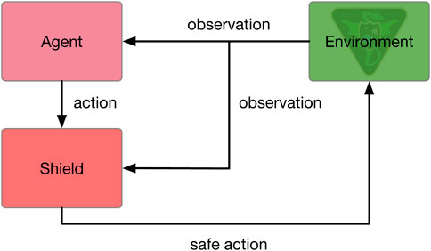
FIGURE 3. Shielded agent-environment interface.

3.4.2 Multi-sensor EOS shield

To create the shield, a safety MDP is derived as described by Harris and Schaub (Harris, 2021; Harris et al., 2021). The safety MDP discretizes the state space to reduce dimensionality to several safety states. The state space of the safety MDP is defined as follows:

${\mathcal{S}}_{\text{safety}}={\mathcal{S}}_{\text{tumbling}}\times {\mathcal{S}}_{\text{saturated}}\times {\mathcal{S}}_{\text{low\hspace{0.17em}power}}(18)$

The safety states take a Boolean value of 0 or 1 on whether the relevant resource state variables are above or below a safety limit. When the safety MDP achieves a nominal state (s_i = (0, 0, 0)), meaning that any action can be safely taken, or if the safety MDP indicates the satellite is tumbling only (s_i = (1, 0, 0)), the action from PPO is passed through. However, if the safety MDP is in any other safety state, the action from PPO is overridden with a safe action. The safety states are defined as follows:

$s_{\text{tumbling}}={\Vert }^{\mathcal{B}}{\mathit{\omega }}_{\mathcal{B}/\mathcal{N}}\Vert \ge 1\text{e}-2\text{\hspace{0.17em}rad/s}(19)$

$s_{\text{saturated}}=\Vert \mathbf{\Omega }\Vert /{\mathrm{\Omega }}_{\text{max}}\ge 0.8(20)$

$s_{\text{low\hspace{0.17em}power}}=\text{battery/max\hspace{0.17em}storage}\le 0.2(21)$

To ensure the safe action is taken, a policy is generated for the safety MDP that guarantees a resource constraint failure does not occur if the safe action is taken. The MDP safety limits and policy actions are both hand tuned and benchmarked to ensure no failures occur. The policy is provided in Table 1.

TABLE 1

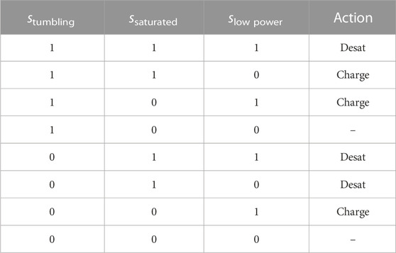
TABLE 1. Multi-Sensor EOS shield policy.

3.4.3 Agile EOS shield

A shield policy is developed for the agile EOS scheduling problem following the same methodology. The key difference in the agile EOS scheduling problem is the addition of the data buffer resource, which is now reflected in the safety MDP. The state space of the safety MDP is defined as follows:

${\mathcal{S}}_{\text{safety}}={\mathcal{S}}_{\text{tumbling}}\times {\mathcal{S}}_{\text{saturated}}\times {\mathcal{S}}_{\text{low\hspace{0.17em}power}}\times {\mathcal{S}}_{\text{buffer\hspace{0.17em}overflow}}(22)$

The safety states are defined as follows:

$s_{\text{tumbling}}={\Vert }^{\mathcal{B}}{\mathit{\omega }}_{\mathcal{B}/\mathcal{N}}\Vert \ge 1\text{e}-2\text{\hspace{0.17em}rad/s}(23)$

$s_{\text{saturated}}=\Vert \mathbf{\Omega }\Vert /{\mathrm{\Omega }}_{\text{max}}\ge 0.6(24)$

$s_{\text{low\hspace{0.17em}power}}=\text{battery/max\hspace{0.17em}storage}\le 0.25(25)$

$s_{\text{buffer\hspace{0.17em}overflow}}=\text{buffer/max\hspace{0.17em}storage}\ge 0.95(26)$

Some of the safety limits that are present for both the multi-sensor EOS and agile EOS scheduling problems are different, which is due to slightly different simulation parameters in the Agile EOS scheduling problem. The policy is provided in Table 2, and is identical to the one developed by Herrmann and Schaub in Reference (Herrmann and Schaub, 2020).

TABLE 2

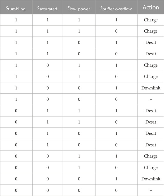
TABLE 2. Agile EOS shield policy.

3.5 MCTS-train

MCTS-Train is a reinforcement learning training pipeline inspired by AlphaGo Zero (Silver et al., 2017). Instead of using an artificial neural network to conduct or replace rollouts in MCTS, MCTS-Train uses a high quality rollout policy within MCTS to generate good estimates of the state-action value function, which are regressed over to produce Q_θ(s, a). The full algorithm for MCTS-train may be found in Algorithm 4. MCTS-Train first generates a training data set of state-action value estimates, $\widehat{Q}(s,a)$, by solving the EOS scheduling problem for hundreds or thousands of unique initial conditions using Monte Carlo Tree Search (Kochenderfer, 2015). For each unique initial condition, MCTS builds a search tree by simulating hundreds of interactions with the environment. A state-action value estimate is maintained as MCTS steps through the environment, which is exploited to select the next best action after a pre-determined number of simulations have been executed. MCTS also utilizes a rollout policy to help it find promising areas to search while building the search tree. The shielded policies presented in Tables 1 and 2 are used as the rollout policies for the multi-sensor EOS and agile EOS scheduling problems, respectively. However, when the safety MDP achieves one of the nominal states, an imaging or downlink mode is initiated instead, depending on the problem.

Algorithm 4.MCTS-Train algorithm.

 1: Initialize set of training data, Q

 2: for iteration 1: N 

 3: for iteration 1: |I| 

 4:  a_i = MCTS.selectAction (s_i)

 5:  s_i+1, r_i ∼ G (s_i, a_i)

 6: Add $\widehat{Q}(s_i,a_i)$ from MCTS to Q

 7: Initialize set of hyperparameters

 8: Initialize empty set of networks, Q_θ

 9: for $\text{hp}\in \text{hyperparameters}$

  10: initialize Q_θ with hp

  11: Q_θ.train (hp)

  12: Q_θ ∪ {Q_θ}

  13: for $Q_{\theta }\in {\mathbf{Q}}_{\theta }$

  14: reward_sum = 0

  15: for iteration 1: |I| 

  16:  $a_i={\text{arg}\text{max}}_{a_i}{Q}_{\theta }$(s_i, a_i)

  17:  s_i+1, r_i ∼ G (s_i, a_i)

  18:  reward_sum + = r_i

  19: Save performance metrics

After the training data is generated, supervised learning is applied over the training data set to generate a neural network approximation of the state-action value function, Q_θ(s, a). Hyperparameters that relate to the activation function, width and depth of the network, learning rate, number of training epochs, etc., can be input into the algorithm to produce a number of neural networks. In this work, mean squared error is used for the loss function,

$L\left(\theta \right)=\frac{1}{|\mathbf{Q}|}{\displaystyle \sum _{s_i\in \mathbf{Q}}}{\left(Q_{\theta }\left(s_i,a_i\right)-\widehat{Q}\left(s_i,a_i\right)\right)}^2\text{,}(27)$

and the Adam optimizer is selected as the optimization algorithm to update the weights of the network(s). After the neural networks are trained, they are validated in the environment using the policy in Eq. 28. Each neural network is executed on the same set of 100 initial conditions and performance metrics are gathered.

$\pi \left(s\right)=\underset{a}{\text{arg}\text{max}}{Q}_{\theta }\left(s,a\right)(28)$

3.6 Genetic algorithm

The final method implemented in this work is the genetic algorithm (GA). The purpose of the GA is to create a benchmark solution to compare the reinforcement solutions against. GAs can be used to schedule spacecraft tasks in an offline manner, but are too slow for on-board implementation, especially if a complex simulator is used. The genetic algorithm is not a reinforcement learning algorithm, but a meta-heuristic optimization algorithm that can be applied to the EOS scheduling problem. It is not guaranteed to solve for the globally optimal solution, but in practice can be tuned to produce good performance. The genetic algorithm is inspired by the biological processes of evolution and natural selection. The genetic algorithm begins by initializing a population of individuals, each of which is a sequence of actions for the EOS scheduling problem. Each individual is evaluated using a fitness function, which is simply the reward function of the corresponding EOS scheduling problem. The population of individuals then mates, and then their offspring are mutated. The offspring are then added to the overall population, and a selection operator is applied to select the best individuals within the population. This process repeats for a specified number of generations. Due to the nondeterministic nature of the genetic algorithm, the population size and number of generations must be sized ensure that a good sample of initial individuals is created and that these individuals have enough generations to mate and mutate into good solutions. The pseudocode for the genetic algorithm is provided in Algorithm 5.

Algorithm 5.Genetic algorithm.

 1: Initialize population

 2: Evaluate fitness of each individual in population

 3: for generation 1: N 

 4: Generate offspring by mating and mutating population

 5: Evaluate offspring

 6: Add offspring to population

 7: Perform selection on population and offspring

The DEAP evolutionary computational framework is used to implement the genetic algorithm⁷. The DEAP framework has a number of pre-defined operators for selection, mating, and mutation. A one point crossover with a probability of 0.25 is used for mating. The selection operator utilized is the selection tournament in which the best individual from three individuals is returned. The population mates using a one point crossover operator, and the population mutates using a uniform mutation operator where each sequence has a 0.25 probability of mutating, and each attribute of a mutating sequence has a 0.3 probability of mutating.

3.7 Basilisk reinforcement learning package

The environments, algorithms (i.e., MCTS-Train, rollout policies, and shields), and algorithm interfaces (i.e., the scripts that setup and run SB3 and DEAP algorithms) are all provided in the bsk_rl Python library⁸. The environments are all contained within the env/ directory. Each environment includes a Gymnasium interface file and a Basilisk simulation file. The Gymnasium interface sends actions to the Basilisk simulation, which turns on or off certain models and tasks. Implementations of MCTS, the genetic algorithm, and the rollout policies are provided within the agents/ directory. Furthermore, the training/ directory includes the scripts that interface with the Stable-Baseline3 package to train PPO, SPPO, A2C, and DQN agents. Various examples for each algorithm are contained within the examples/ directory, which others may use as a starting point to implement and compare their own reinforcement learning algorithms and spacecraft scheduling problems. Finally, the utilities/ directory contains various utility functions that are used throughout the library. Authors wishing to make contributions to the bsk_rl library are encouraged to do so, and issues can be made directly in the GitHub repository.

4 Results

In this section, each reinforcement learning algorithm is benchmarked in each environment and compared to one another on the basis of performance, performance variance, and wall clock time. First, the hyperparameters of both Monte Carlo tree search and the genetic algorithm are tuned to ensure each of the algorithms are performing well given the available computing power. These results can also provide baseline performance metrics for the reinforcement learning algorithms.

Past work tunes the hyperparameters regarding the activation function, number of training epochs, learning rate, batch size, dropout, loss function, and optimizer for the supervised learning portion of MCTS-Train (Herrmann and Schaub, 2021; Herrmann and Schaub, 2023a). The optimized hyperparameters are fixed in each MCTS-Train experiment and are summarized in Table 3. The Leaky ReLU activation function is used for each hidden layer. The activation function is defined as follows:

$\text{Leaky\hspace{0.17em}ReLU}\left(x\right)=\left\{\begin{array}{cc}x\hfill & \text{if\hspace{0.17em}}x\ge 0\hfill \\ \alpha x\hfill & \text{otherwise}\hfill \end{array}\right.(29)$

TABLE 3

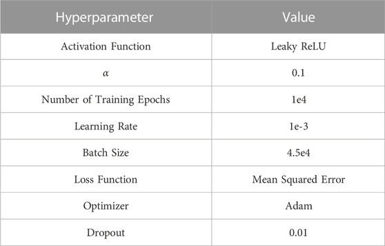
TABLE 3. Optimized hyperparameters for MCTS-Train.

Each network is trained for a maximum of 10,000 epochs with a batch size of 45,000 to ensure stable convergence. The Adam optimizer with an initial learning rate of 1e-3 is utilized. The mean squared error loss function is used to train each network. Furthermore, a small amount of dropout is added to each hidden layer to help prevent overfitting. The probability of dropout is 0.01.

The hyperparameters of each SB3 algorithm (PPO, SPPO, A2C, and DQN) are tuned using a two-step process. In the first step, parameters such as the batch size, number of steps before an update, number of training epochs, etc., are optimized for a network with 4 hidden layers and 20 nodes per hidden layer. The parameters are optimized for relatively small networks because larger networks have a tendency to be quite forgiving for some algorithms. The optimized hyperparameters are provided in Table 4. For PPO and SPPO, a search is performed over the batch size and number of training epochs, as these parameters produce the largest changes in performance. Performance is most dependent on the number of epochs (the number of times that each data point is regressed over with the policy). More epochs typically result in better performance, but this comes at a computational cost. All other parameters are kept as the default parameters for both PPO and SPPO. For A2C, a search is performed over the learning rate and the number of steps before an update. Smaller learning rates are preferred because larger learning rates result in unstable performance. Furthermore, a smaller number of steps before an update is also preferred. This is somewhat of a proxy for PPO’s number of training epochs and the batch size. A smaller number of steps before update means a smaller batch size and more opportunities to update the policy. For DQN, the batch size and buffer size are tuned. These parameters are constant among each problem. Each algorithm utilizes the Leaky ReLU activation function with the same α parameter in Table 3. However, no dropout is utilized for these algorithms. In the second step, these optimized hyperparameters are deployed in a search over the number of hidden layers and the number of nodes per hidden layer. For PPO and shielded PPO, only one policy is trained for each hyperparameter combination because the algorithms are relatively stable. For A2C and DQN, five policies are trained and evaluated because the performance of the algorithms can vary widely between different seeds.

TABLE 4

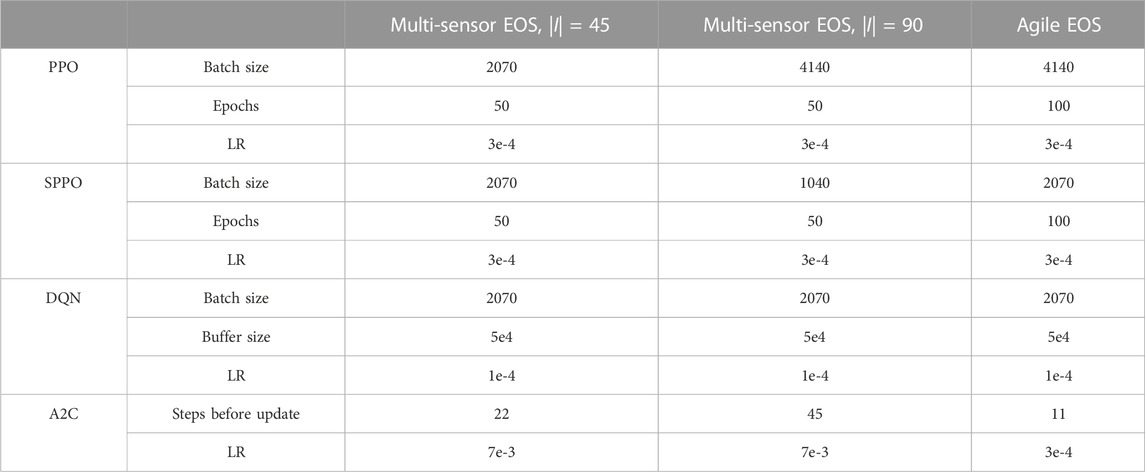
TABLE 4. Optimized hyperparameters for SB3 algorithms.

After the benchmarks are presented over the number of hidden layers and nodes for MCTS-Train and the SB3 algorithms, the optimized hyperparameters are selected for each algorithm and the algorithms are benchmarked once more. Five trials of training are performed for each algorithm. The training curves with variance between trials are evaluated to determine how quickly each algorithm converges and how much the algorithms can vary in performance between seeds.

4.1 MCTS hyperparameter searches

Before MCTS can be used to generate training data, the hyperparameters of MCTS must be tuned. The two tunable hyperparameters of MCTS are the number of simulations-per-step and the exploration constant. The number of simulations-per-step is the number of simulations MCTS runs per step through the environment. The more simulations-per-step, the better the state-action value estimate. The exploration constant is used to scale the exploration term in MCTS, which is the square root of the log of the number of times a state has been visited divided by the number of times the state-action pair has been visited. The exploration constant is used to balance exploration and exploitation. The higher the exploration constant, the more exploration is favored.

For each EOS scheduling problem, each combination of [5, 10, 20, 40, 80] simulations-per-step and [0.1, 0.5, 1, 2, 4] exploration constant are deployed for 30 trials. The results of the hyperparameter search are shown in Figure 4, where the solid line represents the average reward across the 30 trials and the transparent highlighting represents the 95% confidence intervals. For each EOS scheduling problem, higher exploration constants result in higher rewards. The number of simulations-per-step also has a significant effect on performance, but after a certain number there are depreciating returns for adding more simulations. This is especially true for the multi-sensor EOS scheduling problem with 45 decision-making intervals and the agile EOS scheduling problem, which also has 45 decision-making intervals. Simulations beyond 20 or so simulations-per-steps adds little improvement. For the multi-sensor EOS scheduling problem with 90 decision-making intervals, this is not necessarily true. The large confidence interval bounds and spread between the exploration constants suggests that even more simulations-per-step could be beneficial. However, the computational cost of running MCTS increases linearly with the number of simulations-per-step, so additional steps are not added.

FIGURE 4

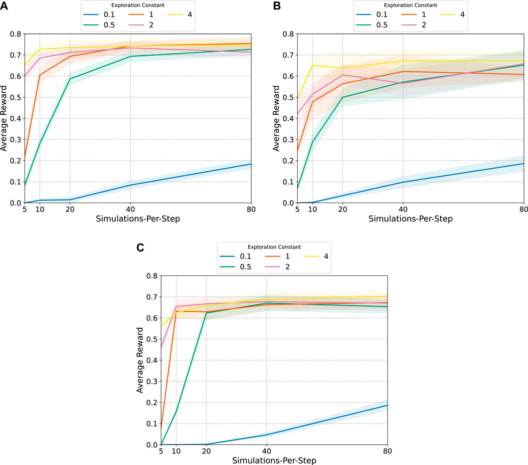
FIGURE 4. MCTS hyperparameter search results: average reward with 95% confidence intervals. (A): Multi-sensor EOS scheduling problem with 45 decision-making intervals. (B): Multi-sensor EOS scheduling problem with 90 decision-making intervals. (D): Agile EOS scheduling problem.

The results in Figure 4 also provide an indication for the performance that can be expected from the RL algorithms. The multi-sensor EOS scheduling problem with 45 decision-making intervals appears to have a maximum reward between 0.7–0.75. The multi-sensor EOS scheduling problem with 90 decision-making intervals appears to have a maximum reward between 0.6–0.7. The same is true for the agile EOS scheduling problem.

4.2 Genetic algorithm hyperparameter searches

The genetic algorithm is implemented for each EOS scheduling problem and benchmarked for various population sizes and generations to ensure the GA is correctly parameterized. A large enough population size is required to increase the probability to genetic algorithm will start with decent individuals that can then be evolved over many generations to produce better offspring. These hyperparameter searches are presented alongside the benchmarks of the RL algorithms in Figures 6F, 7F, 8F, and discussed in relation to the RL benchmarks in the corresponding sections. In comparison to the MCTS benchmarks in Figure 4, the GA is able to match the performance for the multi-sensor EOS scheduling problem. The GA performs slightly worse than MCTS for the agile EOS scheduling problem for the number of generations and population sizes explored. More computation could close the performance gap, but at a computational cost. These results highlight some of the pitfalls of using a genetic algorithm for EOS scheduling. The algorithm is not guaranteed to find a globally optimal solution, and its stochastic nature necessitates a large population size and number of generations to ensure a good solution is found.

An example convergence curve for the genetic algorithm is provided in Figure 5. In this curve, a genetic algorithm with a population size of 400 is run for 400 generations on the agile EOS scheduling problem. The genetic algorithm converges to a good solution in the first 50 generations, largely due to the large population size. The genetic algorithm then continues to improve the solution over the next 350 generations, but the improvement is marginal.

FIGURE 5

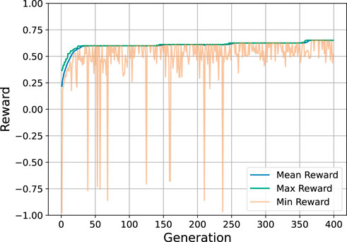
FIGURE 5. Example convergence curve for the genetic algorithm.

4.3 Multi-sensor EOS benchmarks

Each algorithm described in Section 3 is benchmarked for two versions of the multi-sensor EOS scheduling problem, one with 45 decision-making intervals (|I| = 45) and one with 90 decision-making intervals (|I| = 90). In the former case, there are 25 total targets in the set T. In the latter case, there are 50 total targets in the set T. Multiple decision-making intervals are evaluated to determine the effect on the trained policies for each algorithm.

4.3.1 45 decision-making intervals

The results for the hyperparameter searches of each algorithm are presented in Figure 6. MCTS-Train is benchmarked for networks with [1, 2, 4] hidden layers and [10, 20, 40, 80, 160, 320, 640] nodes per hidden layer. The SB3 algorithms (PPO, SPPO, A2C, and DQN) are benchmarked for networks with [1, 2, 4] hidden layers and [10, 20, 40, 80, 160] nodes per hidden layer because performance does not tend to improve outside of these more limited parameters. Conversely, MCTS-Train sometimes benefits from few hidden layers but many nodes per hidden layer. Finally, the GA is benchmarked for [100, 200, 400] generations and population sizes of [100, 200, 400]. This range of parameters is sufficient to provide a good benchmark.

FIGURE 6

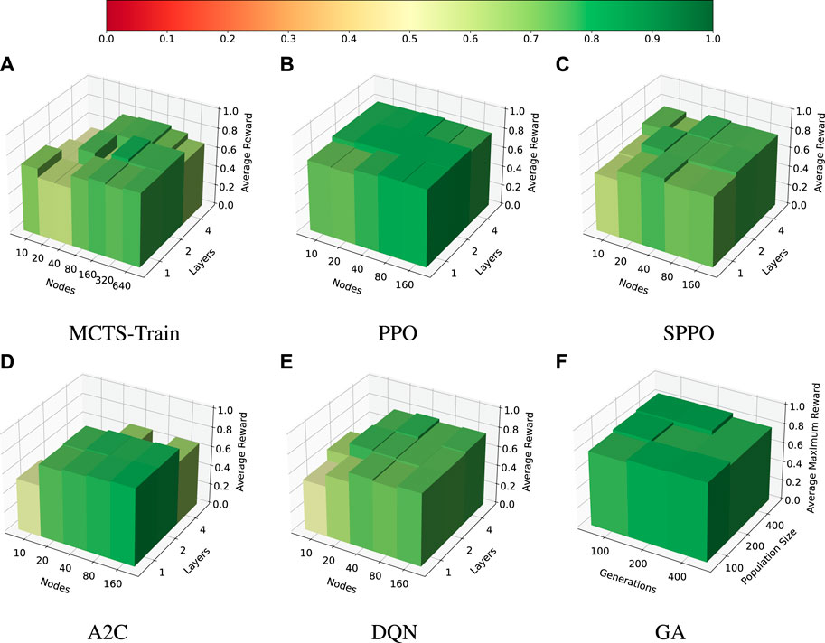
FIGURE 6. Multi-sensor EOS scheduling problem, |I| = 45. The average reward for each hyperparameter combination is displayed for each algorithm. (A): MCTS-Train. (B): PPO. (C): SPPO. (D): A2C. (E): DQN. (F): GA.

After each policy is trained for MCTS-Train and the SB3 algorithms, the performance of each is evaluated in the environment with approximately 150 trials. The genetic algorithm hyperparameter search is performed with only 20 trials for each hyperparameter combination. In this case, the genetic algorithm provides the upper bound on performance at around 0.8 average reward across all numbers of generations and population size. Each of the other algorithms is able to compute policies that are close to this upper bound. PPO is shown to be extremely stable over the entire range of network size hyperparameters selected and produces the best performance of all the RL algorithms across the board. Shielded PPO is shown to be slightly less stable and performant than PPO, but produces a policy that is close to the upper bound that never violates the resource constraints due to the shield. PPO itself is not guaranteed to never produce resource constraint violations, but it is easier for the algorithm to find high-performing policies. MCTS-Train, DQN, and A2C are typically able to produce good performing policies, but are shown to be less stable than PPO and shielded PPO. Furthermore, MCTS-Train requires much larger network sizes to produce high performing policies. The maximum number of nodes evaluated for MCTS-Train is 640, compared to just 160 from the other algorithms. At face value, this study would indicate that PPO is marginally better than the other RL algorithms. However, the number of decision-making intervals utilized in this experiment is relatively small.

4.3.2 90 Decision-making intervals

An identical experiment is performed for the multi-sensor EOS scheduling problem with 90 decision-making intervals. This experiment is performed to determine how the size of the search space impacts performance. The hyperparameters swept over in this experiment are the exact same as those in the previous experiment for each algorithm. However, there are slight differences in the hyperparameters regarding batch size, epochs, etc. The results of this search are presented in Figure 7.

FIGURE 7

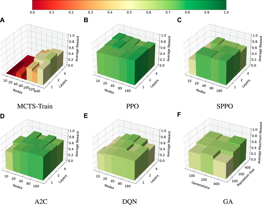
FIGURE 7. Multi-sensor EOS scheduling problem, |I| = 90. Average reward for the selected hyperparameters of each algorithm. (A): MCTS-Train. (B): PPO. (C): SPPO. (D): A2C. (E): DQN. (F): GA.

In this case, both the genetic algorithm and MCTS-Train are capable of producing good performance, but in general struggle to match the performance of the other algorithms. MCTS-Train is only able to find one policy that achieves more than 0.5 average reward. The reason for this is that both of these algorithms are searching over the action space to find optimal policies. The total number of possible trajectories through the environment is $|\mathcal{A}{|}^{|I|}$. 90 decision-making intervals results in vastly more possible trajectories, which makes it more difficult for these algorithms to find good solutions. This indicates that the genetic algorithm and MCTS-Train may not be well suited if a long planning horizon is desired, i.e., training for a full day or a full week of operations. PPO, SPPO, and A2C are shown to be the most stable and performant algorithms. They are all able to produce good performing policies as they are optimizing over the state space instead. Furthermore, these are all policy gradient algorithms, which might also help explain why they perform better. DQN’s performance is more on par with the genetic algorithm or the best case scenario for MCTS-Train, but is certainly worse than the performance of DQN on the 45 decision-making interval version of the multi-sensor EOS scheduling problem. Regardless of the degradation in performance, DQN is fairly stable over the selected hyperparameters, which MCTS-Train is not. MCTS-Train is likely unstable for this problem because MCTS has not properly converged, as demonstrated by the large confidence intervals and spreads between hyperparameters in Figure 4B. Again, this indicates that MCTS-Train may not work well for long planning horizons. PPO, SPPO, A2C, and DQN could all be trained on even longer decision-making intervals without much increase in computational complexity provided that the same number of steps are used for each. However, DQN is likely not a good candidate as the number of decision-making intervals increases, as evidenced by the reduction in performance in the 90 decision-making interval version of the multi-sensor EOS scheduling problem.

4.4 Agile EOS benchmarks

A final hyperparameter experiment is performed for the agile EOS scheduling problem. The results are presented in Figure 8. The same MCTS-Train and genetic algorithm hyperparameter combinations used in the last two experiments are again used in this one. However, the sizes of the neural networks for the SB3 algorithms are increased to ensure a large enough search space is explored. The SB3 algorithms are benchmarked for [1, 2, 4] hidden layers and [10, 20, 40, 80, 160, 320, 640] nodes per hidden layer.

FIGURE 8

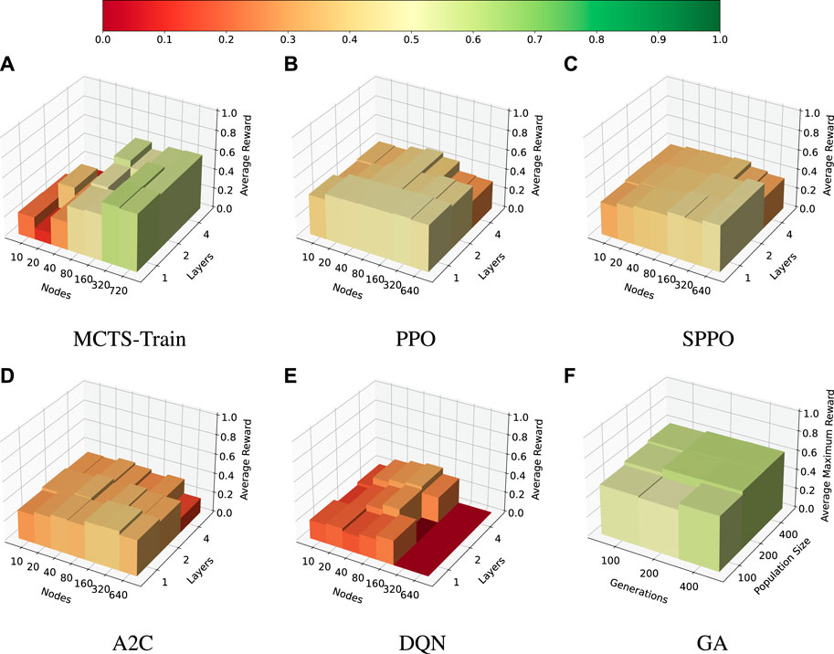
FIGURE 8. Agile EOS scheduling problem. Average reward for the selected hyperparameters of each algorithm. (A): MCTS-Train. (B): PPO. (C): SPPO. (D): A2C. (E): DQN. (F): GA.

In this case, only MCTS-Train and the genetic algorithm are able to produce high-performing policies. Each of the other algorithms converges to some locally maximal policy. PPO, SPPO, and A2C are shown to be the most stable, while DQN is shown to have large instability and poor robustness for neural networks with more than 160 nodes per hidden layer. The reason for the relatively poor performance of the SB3 algorithms is likely due to the fact that the agile EOS scheduling problem is more complex than the multi-sensor EOS scheduling problem in terms of resource management and science objectives. The agile EOS scheduling problem has a more complex reward function, an additional resource constraint, more sparse reward, and a larger action space. MCTS-Train is able to leverage its high quality rollout policy, which initially finds a safe trajectory of actions that MCTS can improve upon. The state-action value estimates produced by MCTS are closer to the optimal state-action value function, which are then regressed over using the artificial neural networks. While a similar shield is used within shielded PPO, shielded PPO ultimately bounds the decision-making agent’s actions to the safety states. MCTS, however, allows the agent to explore actions that may violate these safety limits with exceeding the limits used within the reward function. When this difference in performance is compared to the multi-sensor EOS scheduling problem results, it is evident that MCTS-Train may be an excellent choice of algorithm as long as the number of decision-making intervals is not too large. A key question that remains, however, is how the EOS scheduling problems formulated in this work translate to real-world EOS scheduling problems with larger data buffers and less aggressive momentum buildup. If the problems can be scaled such that only 45 decision-making intervals are required to sufficiently model the problem, MCTS-Train may make an excellent choice of algorithm due to its ability to handle many resource constraints and complex science objectives.

4.5 Performance variance

To evaluate the consistency of each algorithm between different training runs and network initializations, a performance variance experiment is performed. For PPO, SPPO, A2C, and DQN the best performing hyperparameters in step one of the optimization process are deployed for five trials of training, each with different initial random seeds. The number of hidden layers is set to 4, and the number of nodes per hidden layer is set to 20. The rest of the hyperparameters are provided in Table 4. For MCTS-Train, the best-performing network hyperparameter combination is selected for the five trials. The genetic algorithm is not considered in this experiment as the results from the GA are not generalized with a neural network. The average reward curves with 1σ standard deviation for each algorithm and each problem are plotted in Figure 9. PPO and SPPO are shown to produce the smallest standard deviation between policies and converge the quickest. This result is not necessarily surprising, as Reference (Schulman et al., 2017) touts PPO as being a reliable algorithm needing little hyperparameter tuning. This claim is also backed up with the hyperparameter searches presented within this work that find that vanilla PPO is extremely stable across the range of hyperparameters. SPPO is not as stable as PPO over the entire range of hyperparameters, but is found to be very stable when a good hyperparameter combination is selected. This is likely due to the fact that it is more difficult to find a high-performing policy that avoids the limits of the safety MDP. A fundamental trade-off exists between resource utilization and science collection. In contrast to the other algorithms, A2C and DQN are shown to be more unstable both across the entire range of hyperparameters and between different runs of the same hyperparameters, particularly for $<$1e4 episodes. As a result, they take longer to converge. In fact, the maximum number of episodes in Figure 9 is primarily driven by these two algorithms. Finally, MCTS-Train is shown to have a very small variance between the different network seeds for the same hyperparameters. While MCTS-Train can be relatively unstable across the entire range of hyperparameters, it is on par with PPO and SPPO in terms of stability when optimized hyperparameters are utilized. When examining the performance variance of each algorithm in addition to the performance across the hyperparameters presented in the last section, it is evident that PPO, SPPO, and MCTS-Train should be among the top candidates for solving EOS scheduling problems. However, MCTS-Train should only be used in cases where the number of decision-making intervals is reasonable (i.e., |I| ≤ 45).

FIGURE 9

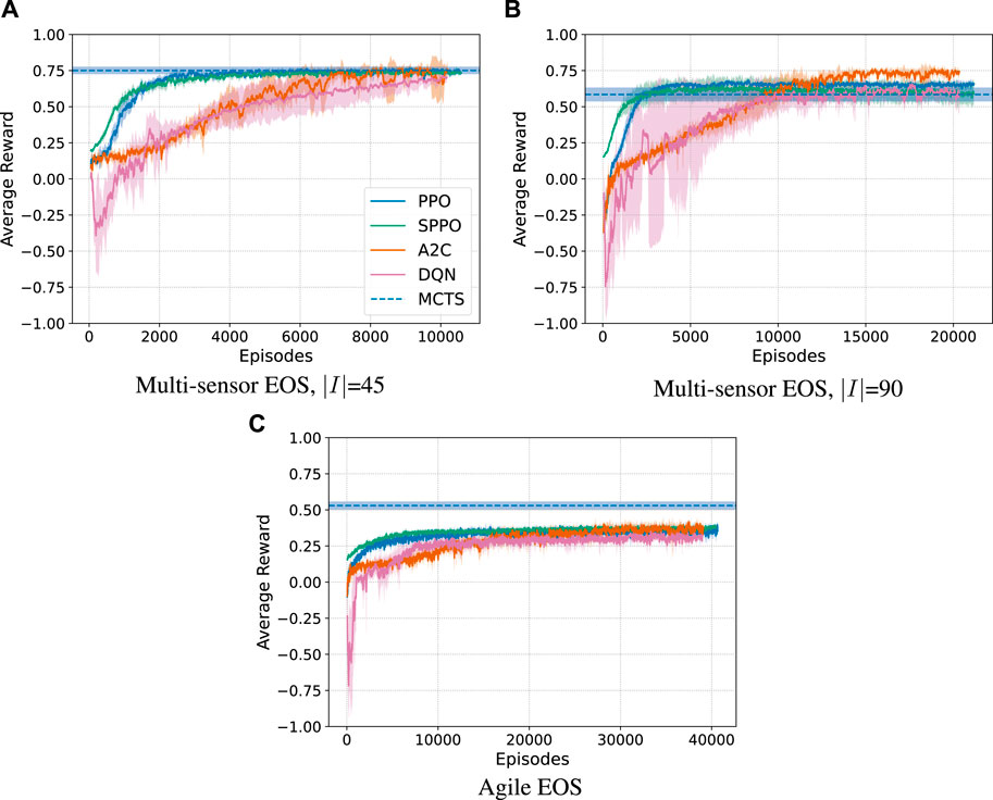
FIGURE 9. Average reward and 1σ standard deviation across 5 trials using the optimized hyperparameters for each algorithm. (A): Multi-sensor EOS, |I| = 45. (B): Multi-sensor EOS, |I| = 90. (D): Agile EOS.

4.6 Wall clock time

The wall clock times for each algorithm using the hyperparameters in Section 4.5 are displayed in Figure 10. The computational experiments resulting in these wall clock times were performed on an AMD 3960X Threadripper CPU with 64 GB of RAM and an NVIDIA 3070 graphics card. The wall clock times in Figure 10A are for the total number of episodes for each algorithm, and the wall clock times in Figure 10B are capped at 10,000 episodes. MCTS-Train is the most computationally expensive algorithm because of the amount of data generated and the number of neural networks produced during the training process. Furthermore, MCTS requires that the Basilisk simulation is rewound by stepping through the trajectory of past actions to create a new child node during the simulation step. This results in a lot of wasted computation. On average, half of the trajectory of executed actions during tree generation are wasted. If Basilisk simulations can be deep copied at the Python level in the future, which could be made possible by moving away from SWIG, then this computational performance could be drastically improved (likely at the cost of increased RAM utilization). Until this happens, MCTS-Train should only be used for complex problems that other algorithms struggle to generate high-performing policies for. PPO, A2C, and DQN are typically in the same ballpark computationally, with the relative performance dependent on the specific problem. In comparison to MCTS-Train, they are single trajectory algorithms that do not rely on building a search tree, so they do not suffer from the need to rewind the simulation in the same manner. SPPO is the least computationally expensive algorithm. The reason for this is that SPPO guarantees that resource constraint violations do not occur during execution. When a resource constraint violation occurs for any of the SB3 algorithms, the simulation is reset, meaning that an entire new target set must be generated by executing a Basilisk simulation and computing access times to construct the list of targets. This is an expensive procedure. Because the SB3 algorithms are synchronous implementations, all of the workers must wait until the reset environment is ready to step through the environment again before they can begin stepping again. As a result, overall CPU utilization decreases and wall clock time increases. Therefore, future works may want to consider using asynchronous implementations of these algorithms. The risk of this is potentially giving up the performance and stability of the SB3 implementations.

FIGURE 10

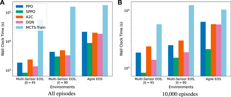
FIGURE 10. Wall clock times associated with each algorithm. Times are displayed for all episodes used in Figure 9 and for 10,000 episodes. (A): All episodes. (B): 10,000 episodes.

5 Conclusion

This paper investigates the performance of different reinforcement learning algorithms applied to EOS scheduling. PPO and SPPO demonstrate exceptional stability and performance, swiftly converging to superior policies in various experiments. While A2C and DQN generally yield high-performing policies, they exhibit considerable variations for different seeds using the same set of hyperparameters. MCTS-Train excels in generating effective policies for the majority of problems, yet faces challenges when dealing with long planning horizons. Furthermore, MCTS-Train is the most computationally expensive algorithm benchmarked. The outcomes of this study offer valuable insights for choosing reinforcement learning algorithms for spacecraft planning and scheduling problems with resource constraints. PPO and SPPO are the recommended algorithms for simple EOS scheduling problems due to their performance and stability across hyperparameters and training runs. MCTS-Train is recommended if challenging EOS scheduling problems are pursued, like the agile EOS scheduling problem in this work. However, this will come at a high computational cost, especially if the simulator cannot be saved off in memory and copied during branching. Future work should investigate how the problems in this work can be deployed in longer operational scenarios with more realistic rates and limits for resource constraint consumption. The algorithms and environments used within this work may be found on the develop branch of the bsk_rl library. We hope other authors will use this library to benchmark their own algorithms and environments, expanding on these comparisons to further the field of reinforcement learning for spacecraft planning and scheduling in a more standardized way.

Data availability statement

The raw data supporting the conclusion of this article will be made available by the authors, without undue reservation.

Author contributions

AH: Conceptualization, Formal Analysis, Investigation, Methodology, Project administration, Software, Writing–original draft. HP: Conceptualization, Methodology, Software, Supervision, Writing–review and editing.

Funding

The author(s) declare financial support was received for the research, authorship, and/or publication of this article. This work is supported by the NASA Space Technology Research Graduate Opportunity (NSTGRO) under Grant 80NSSC20K1162. This work is also partially supported by the Air Force STTR Program, FA8649-22-P-0833. This work utilized the Alpine high performance computing resource at the University of Colorado Boulder. Alpine is jointly funded by the University of Colorado Boulder, the University of Colorado Anschutz, Colorado State University, and the National Science Foundation (award 2201538).

Conflict of interest

The authors declare that the research was conducted in the absence of any commercial or financial relationships that could be construed as a potential conflict of interest.

Publisher’s note

All claims expressed in this article are solely those of the authors and do not necessarily represent those of their affiliated organizations, or those of the publisher, the editors and the reviewers. Any product that may be evaluated in this article, or claim that may be made by its manufacturer, is not guaranteed or endorsed by the publisher.

Footnotes

¹https://github.com/AVSLab/bsk_rl

²https://hanspeterschaub.info/basilisk

³https://gymnasium.farama.org/

⁴https://stable-baselines3.readthedocs.io/en/master/modules/dqn.html

⁵https://stable-baselines3.readthedocs.io/en/master/modules/a2c.html

⁶https://stable-baselines3.readthedocs.io/en/master/modules/ppo.html

⁷https://deap.readthedocs.io/en/master/index.html

⁸https://github.com/AVSLab/bsk_rl

References

Alshiekh, M., Bloem, R., Ehlers, R., Könighofer, B., Niekum, S., and Topcu, U. (2018). Safe reinforcement learning via shielding. Proc. AAAI Conf. Artif. Intell. 32. doi:10.1609/aaai.v32i1.11797

CrossRef Full Text | Google Scholar

Bernard, D. E., Dorais, G. A., Fry, C., Gamble, E. B., Kanefsky, B., Kurien, J., et al. (1998). Design of the remote agent experiment for spacecraft autonomy. IEEE Aerosp. Conf. Proc. 2, 259–281. doi:10.1109/AERO.1998.687914

CrossRef Full Text | Google Scholar

Bernard, D., Dorais, G., Gamble, E., Kanefsky, B., Kurien, J., Man, G. K., et al. (1999). Spacecraft autonomy flight experience: the ds1 remote agent experiment. Proc. AIAA 1999, 28–30. doi:10.2514/6.1999-4512

CrossRef Full Text | Google Scholar

Blacker, P., Bridges, C. P., and Hadfield, S. (2019). “Rapid prototyping of deep learning models on radiation hardened cpus,” in 2019 NASA/ESA Conference on Adaptive Hardware and Systems (AHS), Colchester, UK, 22-24 July 2019, 25–32.

CrossRef Full Text | Google Scholar

Chien, S., Doubleday, J., Thompson, D. R., Wagstaff, K., Bellardo, J., Francis, C., et al. (2016). Onboard autonomy on the intelligent payload experiment CubeSat mission. J. Aerosp. Inf. Syst. (JAIS) 14, 307–315. doi:10.2514/1.I010386

CrossRef Full Text | Google Scholar

Chien, S., Mclaren, D., Doubleday, J., Tran, D., Tanpipat, V., and Chitradon, R. (2019). Using taskable remote sensing in a sensor web for Thailand flood monitoring. J. Aerosp. Inf. Syst. 16, 107–119. doi:10.2514/1.I010672

CrossRef Full Text | Google Scholar

Chien, S., Sherwood, R., Tran, D., Cichy, B., Rabideau, G., Castano, R., et al. (2005). Using autonomy flight software to improve science return on earth observing one. J. Aerosp. Comput. Inf. Commun. 2, 196–216. doi:10.2514/1.12923

CrossRef Full Text | Google Scholar

Chien, S. A., Davies, A. G., Doubleday, J., Tran, D. Q., Mclaren, D., Chi, W., et al. (2020). Automated volcano monitoring using multiple space and ground sensors. J. Aerosp. Inf. Syst. 17, 214–228. doi:10.2514/1.I010798

CrossRef Full Text | Google Scholar

Dunkel, E., Swope, J., Towfic, Z., Chien, S., Russell, D., Sauvageau, J., et al. (2022). “Benchmarking deep learning inference of remote sensing imagery on the qualcomm snapdragon and intel movidius myriad x processors onboard the international space station,” in IGARSS 2022-2022 IEEE International Geoscience and Remote Sensing Symposium (IEEE), Kuala Lumpur, Malaysia, 17-22 July 2022, 5301–5304.

CrossRef Full Text | Google Scholar

Dunlap, K., Mote, M., Delsing, K., and Hobbs, K. L. (2023). Run time assured reinforcement learning for safe satellite docking. J. Aerosp. Inf. Syst. 20, 25–36. doi:10.2514/1.i011126

CrossRef Full Text | Google Scholar

Eddy, D., and Kochenderfer, M. (2020). “Markov decision processes for multi-objective satellite task planning,” in 2020 IEEE Aerospace Conference (IEEE), Big Sky, MT, USA, 07-14 March 2020, 1–12.

CrossRef Full Text | Google Scholar

Federici, L., Benedikter, B., and Zavoli, A. (2021). Deep learning techniques for autonomous spacecraft guidance during proximity operations. J. Spacecr. Rockets 58, 1774–1785. doi:10.2514/1.a35076

CrossRef Full Text | Google Scholar

Federici, L., Scorsoglio, A., Ghilardi, L., D’Ambrosio, A., Benedikter, B., Zavoli, A., et al. (2022a). Image-based meta-reinforcement learning for autonomous guidance of an asteroid impactor. J. Guid. Control, Dyn. 45, 2013–2028. doi:10.2514/1.g006832

CrossRef Full Text | Google Scholar

Federici, L., Scorsoglio, A., Zavoli, A., and Furfaro, R. (2022b). Meta-reinforcement learning for adaptive spacecraft guidance during finite-thrust rendezvous missions. Acta Astronaut. 201, 129–141. doi:10.1016/j.actaastro.2022.08.047

CrossRef Full Text | Google Scholar

Fukunaga, A., Rabideau, G., Chien, S., and Yan, D. (1997). “Towards an application framework for automated planning and scheduling,” in 1997 IEEE Aerospace Conference, Snowmass, CO, USA, 13-13 February 1997, 375–386. doi:10.1109/AERO.1997.574426

CrossRef Full Text | Google Scholar

Furfaro, R., Scorsoglio, A., Linares, R., and Massari, M. (2020). Adaptive generalized zem-zev feedback guidance for planetary landing via a deep reinforcement learning approach. Acta Astronaut. 171, 156–171. doi:10.1016/j.actaastro.2020.02.051

CrossRef Full Text | Google Scholar

Gaudet, B., Linares, R., and Furfaro, R. (2020a). Adaptive guidance and integrated navigation with reinforcement meta-learning. Acta Astronaut. 169, 180–190. doi:10.1016/j.actaastro.2020.01.007

CrossRef Full Text | Google Scholar

Gaudet, B., Linares, R., and Furfaro, R. (2020b). Deep reinforcement learning for six degree-of-freedom planetary landing. Adv. Space Res. 65, 1723–1741. doi:10.1016/j.asr.2019.12.030

CrossRef Full Text | Google Scholar

Gaudet, B., Linares, R., and Furfaro, R. (2020c). Terminal adaptive guidance via reinforcement meta-learning: applications to autonomous asteroid close-proximity operations. Acta Astronaut. 171, 1–13. doi:10.1016/j.actaastro.2020.02.036

CrossRef Full Text | Google Scholar

Gaudet, B., Linares, R., and Furfaro, R. (2020d). Six degree-of-freedom body-fixed hovering over unmapped asteroids via lidar altimetry and reinforcement meta-learning. Acta Astronaut. 172, 90–99. doi:10.1016/j.actaastro.2020.03.026

CrossRef Full Text | Google Scholar

Haijiao, W., Zhen, Y., Wugen, Z., and Dalin, L. (2019). Online scheduling of image satellites based on neural networks and deep reinforcement learning. Chin. J. Aeronautics 32, 1011–1019. doi:10.1016/j.cja.2018.12.018

CrossRef Full Text | Google Scholar

Harris, A., Valade, T., Teil, T., and Schaub, H. (2021). Generation of spacecraft operations procedures using deep reinforcement learning. J. Spacecr. Rockets 2021, 1–16. doi:10.2514/1.A35169

CrossRef Full Text | Google Scholar

Harris, A. T. (2021). Autonomous management and control of multi-spacecraft operations leveraging atmospheric forces. Ph.D. thesis. Colorado: University of Colorado at Boulder.

Google Scholar

He, Y., Xing, L., Chen, Y., Pedrycz, W., Wang, L., and Wu, G. (2020). A generic markov decision process model and reinforcement learning method for scheduling agile earth observation satellites. IEEE Trans. Syst. Man, Cybern. Syst. 52, 1463–1474. doi:10.1109/tsmc.2020.3020732

CrossRef Full Text | Google Scholar

Herrmann, A., and Schaub, H. (2020). “Monte Carlo tree search with value networks for autonomous spacecraft operations,” in AAS/AIAA Astrodynamics Specialist Conference, Lake Tahoe, CA. AAS 20-473.

Google Scholar

Herrmann, A., and Schaub, H. (2023a). Reinforcement learning for the agile earth-observing satellite scheduling problem. IEEE Trans. Aerosp. Electron. Syst. 2023, 1–13. doi:10.1109/TAES.2023.3251307

CrossRef Full Text | Google Scholar

Herrmann, A., and Schaub, H. (2023b). “A comparison of deep reinforcement learning algorithms for earth-observing satellite scheduling,” in AAS Spaceflight Mechanics Meeting, Austin, TX. Paper No. AAS 23-116.

Google Scholar

Herrmann, A. P., and Schaub, H. (2021). Monte Carlo tree search methods for the earth-observing satellite scheduling problem. J. Aerosp. Inf. Syst. 19, 70–82. doi:10.2514/1.I010992

CrossRef Full Text | Google Scholar

Hovell, K., and Ulrich, S. (2021). Deep reinforcement learning for spacecraft proximity operations guidance. J. Spacecr. Rockets 58, 254–264. doi:10.2514/1.a34838

CrossRef Full Text | Google Scholar

Hovell, K., and Ulrich, S. (2022). Laboratory experimentation of spacecraft robotic capture using deep-reinforcement-learning–based guidance. J. Guid. Control, Dyn. 45, 2138–2146. doi:10.2514/1.g006656

CrossRef Full Text | Google Scholar

Kenneally, P. W., Piggott, S., and Schaub, H. (2020). Basilisk: a flexible, scalable and modular astrodynamics simulation framework. J. Aerosp. Inf. Syst. 17, 496–507. doi:10.2514/1.i010762

CrossRef Full Text | Google Scholar

Knight, S., Rabideau, G., Chien, S., Engelhardt, B., and Sherwood, R. (2001). Casper: space exploration through continuous planning. IEEE Intell. Syst. 16, 70–75. doi:10.1109/MIS.2001.956084

CrossRef Full Text | Google Scholar

Kochenderfer, M. J. (2015). Decision making under uncertainty: theory and application (Massachusetts institute of Technology), chap. Sequential Problems. Cambridge: MIT press, 102–103.

Google Scholar

Mnih, V., Badia, A. P., Mirza, M., Graves, A., Lillicrap, T., Harley, T., et al. (2016). “Asynchronous methods for deep reinforcement learning,” in International conference on machine learning (PMLR), 1928–1937.

Google Scholar

Mnih, V., Kavukcuoglu, K., Silver, D., Rusu, A. A., Veness, J., Bellemare, M. G., et al. (2015). Human-level control through deep reinforcement learning. Nature 518, 529–533. doi:10.1038/nature14236

PubMed Abstract | CrossRef Full Text | Google Scholar

Muscettola, N., Nayak, P. P., Pell, B., and Williams, B. C. (1998). Remote agent: to boldly go where no ai system has gone before. Artif. Intell. 103, 5–47. doi:10.1016/s0004-3702(98)00068-x

CrossRef Full Text | Google Scholar

Oestreich, C. E., Linares, R., and Gondhalekar, R. (2021). Autonomous six-degree-of-freedom spacecraft docking with rotating targets via reinforcement learning. J. Aerosp. Inf. Syst. 18, 417–428. doi:10.2514/1.i010914

CrossRef Full Text | Google Scholar

Schaub, H., and Junkins, J. L. (2018). Analytical mechanics of space systems. 4th edn. Reston, VA: AIAA Education Series. doi:10.2514/4.105210

CrossRef Full Text | Google Scholar

Schulman, J., Wolski, F., Dhariwal, P., Radford, A., and Klimov, O. (2017). Proximal policy optimization algorithms.

Google Scholar

Scorsoglio, A., D’Ambrosio, A., Ghilardi, L., Gaudet, B., Curti, F., and Furfaro, R. (2022). Image-based deep reinforcement meta-learning for autonomous lunar landing. J. Spacecr. Rockets 59, 153–165. doi:10.2514/1.a35072

CrossRef Full Text | Google Scholar

Silver, D., Schrittwieser, J., Simonyan, K., Antonoglou, I., Huang, A., Guez, A., et al. (2017). Mastering the game of go without human knowledge. Nature 550, 354–359. doi:10.1038/nature24270

PubMed Abstract | CrossRef Full Text | Google Scholar

Sutton, R. S., and Barto, A. G. (2018). Reinforcement learning: an introduction. Cambridge: MIT press.

Google Scholar

Takahashi, S., and Scheeres, D. (2022). Autonomous proximity operations at small neas. 33rd Int. Symposium Space Technol. Sci. (ISTS) 2.

Google Scholar

Zhao, X., Wang, Z., and Zheng, G. (2020). Two-phase neural combinatorial optimization with reinforcement learning for agile satellite scheduling. J. Aerosp. Inf. Syst. 17, 346–357. doi:10.2514/1.i010754

CrossRef Full Text | Google Scholar