A comparison of Fourier and POD mode decomposition methods for high-speed Hall thruster video

Hall thrusters are susceptible to large-amplitude plasma oscillations that impact thruster performance and lifetime and are also difficult to model. High-speed cameras are a popular tool to study these dynamics due to their spatial resolution and are a popular, nonintrusive complement to in situ probes. High-speed video of thruster oscillations can be isolated (decomposed) into coherent structures (modes) with algorithms that help us better understand the evolution and interactions of each. This work provides an introduction, comparison, and step-by-step tutorial on established Fourier and newer Proper Orthogonal Decomposition (POD) algorithms as applied to high-speed video of the unshielded H6 6-kW laboratory model Hall thruster. From this dataset, both sets of algorithms identify and characterize m = 0 and m > 0 modes in the discharge channel and cathode regions of the thruster plume, as well as mode hopping between the m = 3 and m = 4 rotating spokes in the channel. The Fourier methods are ideal for characterizing linear modal structures and also provide intuitive dispersion relationships. By contrast, the POD method tailors a basis set using energy minimization techniques that better captures the nonlinear nature of these structures and with a simpler implementation. Together, the Fourier and POD methods provide a more complete toolkit for studying Hall thruster plasma instabilities and mode dynamics. Specifically, we recommend first applying POD to quickly identify the nature and location of global dynamics and then using Fourier methods to isolate dispersion plots and other wave-based physics.

1 Introduction

The Hall thruster (HT) is a standard spacecraft electric propulsion system that uses crossed electric and magnetic fields $\left(\mathbf{E}\times \mathbf{B}\right)$ to ionize and accelerate propellant (Goebel and Katz, 2008; Boeuf, 2017). Their high specific impulse and technological maturity make them ideal for long duration satellite station keeping and time-insensitive missions, such as orbit raising, with thousands currently in orbit and more planned. However, HTs experience anomalous electron transport across their magnetic field that is not sufficiently understood to permit fully predictive thruster models, motivating continued improvement of diagnostics for model validation. This lack of validation is especially important for increased qualification by simulation for new thruster designs at ever-higher power, such as the N30 or X3 nested Hall thrusters, where full life qualification in a ground test facility would be prohibitively expensive for 10–100 kW thrusters (Florenz et al., 2012; Hall et al., 2017).

Anomalous electron transport has been strongly linked to plasma oscillations in HTs (Choueiri, 2001) in both the thruster discharge channel (Parker et al., 2010; McDonald and Gallimore, 2011a) and cathode regions (Jorns et al., 2020). Long-wavelength azimuthal oscillations, the focus of this work, are typically characterized in a Fourier representation with integer mode numbers, m, including the azimuthally uniform m = 0 “breathing” modes in HT channels (Sekerak et al., 2016; Dale, 2019) and cathodes (Goebel et al., 2007; Georgin et al., 2019), m > 0 azimuthally rotating “spoke” modes in the channel, and a m = 1 counter rotating “anti-drift” modes around the cathode (Jorns and Hofer, 2014). The rotating spoke channel modes, first observed in an early Hall accelerator by Janes and Lowder (Janes and Lowder, 1966), are now known to be ubiquitous in unshielded thrusters (McDonald and Gallimore, 2011b) though they may be less common in magnetically shielded thrusters (Jorns and Hofer, 2014; Baird, 2020). Cathode m = 1 anti-drift modes have been previously observed in both shielded and unshielded versions of the H6 Hall thruster (Jorns and Hofer, 2014) (the unshielded H6 is studied in this work). All of these modes are historically characterized by one or more in situ diagnostics, but the localized nature of these diagnostics both perturb the plasma and make it difficult to relate individual measurements to global mode structures.

High-speed imaging (HSI) has become a popular complementary diagnostic to in situ probes and has proven itself well suited to characterizing mode dynamics (Parker et al., 2010; McDonald and Gallimore, 2013; Jorns and Hofer, 2014). Its popularity is due to its ease of use, nonintrusive nature, high speed (100 s of kHz), and fine spatial resolution of order millimeters per pixel. HSI was first used on HTs to relate image brightness to plasma density oscillations measured by electrical probes (Darnon et al., 1997). This and later work has led to the use of pixel light intensity as a proxy for discharge current (Hara et al., 2014).

To isolate and characterize individual mode dynamics from HSI, various post-processing algorithms have been developed. Early work subtracted the time-average from each pixel to reveal multiple m > 1 modes in the H6 Hall thruster channel (McDonald and Gallimore, 2011b). Later, Fourier techniques were used with azimuthal binning to isolate the frequency spectrum associated with individual channel modes (McDonald M. and Gallimore A., 2011). Fourier methods have also been used to provide azimuthal dispersion plots within the CHT (cylindrical Hall thruster) (Parker et al., 2010) and H6 ¹⁷ thruster channels. A phase-based Fourier analysis was developed to isolate the spatial structure of the m = 1 cathode mode on the H6 thruster (Jorns and Hofer, 2014) and m > 0 channel and cathode modes on the HERMeS thruster (Baird, 2020). An alternative Fourier-based visualization method, Cross-Spectral-Density (CSD), was developed on the CHT thruster (Romadanov et al., 2019).

The Fourier methods remain the most established method for isolating and analyzing Hall thruster plasma oscillations, but they have several disadvantages. First, their linear sine/cosine bases are not ideal for nonlinear features. Second, Fourier methods require several preprocessing steps for high-speed video; this added complexity requires additional computational overhead and makes it more difficult to study multi-dimensional dynamics.

An alternative to Fourier methods are Singular Value Decomposition (SVD) based algorithms (Brunton and Kutz, 2019). The chief advantage of SVD is that it creates a tailored set of bases for each dataset based on the energy (i.e., amplitude) of each coherent dynamic within the measurement instead of assuming a basis (e.g., Fourier’s sines and cosines). This facilitates improved characterization and reconstruction of nonlinear dynamics without making any physical assumptions of the system. SVD also requires minimal preprocessing compared with Fourier methods.

The most notable and likely simplest SVD algorithm is Proper Orthogonal Decomposition (POD) which is extensively used in fluid mechanics (Benner et al., 2015; Taira et al., 2017; Brunton and Kutz, 2019). A classic POD application is to decompose fluid vortex shedding around a body (e.g., a cylinder) into discrete modes (Noack et al., 2003; Oudheusden et al., 2005). POD has also been used in plasma physics to characterize plasma oscillations (Dudok de Wit et al., 1994; Levesque et al., 2013; van Milligen et al., 2014; Hansen et al., 2015; Kaptanoglu et al., 2021) but is often referred to as Biorthogonal Decomposition (BD). Very recently, POD has been used to characterize axial and azimuthal modes in Hall thruster high-speed video (Désangles et al., 2020), azimuthal modes in a hollow cathode plume (Becatti et al., 2021), and study mode coupling in an annular hollow cathode plume (Brooks et al., 2022). More sophisticated SVD algorithms exist, most notably DMD (Dynamic Mode Decomposition) (Schmid, 2010; Tu et al., 2014) and have applications in active control, linear dynamics, and plasma physics (Taylor et al., 2018; Sasaki et al., 2019; Kaptanoglu et al., 2020).

The goal of this work is to compare Fourier and POD techniques as applied to Hall thruster high-speed imaging in a tutorial format. To this end, this work analyzes a high-speed video recording of the unshielded H6 Hall thruster plume and provides a step-by-step explanation of algorithm’s implementation and results. This work starts by introducing the H6 thruster, high-speed video dataset, and video preprocessing in Section 2. Section 3 discusses several established Fourier mode analysis methods and, when applied to the H6 dataset, identifies simultaneous cathode and channel modes in addition to mode hopping within the channel. Section 4 introduces the SVD algorithm and its most common implementation: Proper Orthogonal Decomposition (POD). When applied to the H6 dataset, POD identifies the same mode behavior and provide several improvements over the Fourier methods. When used together, POD and Fourier methods provide a more complete toolkit for identifying and the isolating global mode dynamics. The code and dataset used for this work are available online (Brooks, 2021).

2 Experimental setup

This section covers the experimental hardware (thruster, facility, high-speed camera), the HSI dataset, and common HSI prepossessing techniques.

2.1 Hardware and dataset

This work focuses on a single illustrative operating condition for the unshielded H6 Hall thruster. The H6 is a laboratory model 6-kW thruster (see Figure 1) with a design operating point of 300 V and 20 mg/s (where 1 mg/s ≈ 1 A) on xenon. In this work, we focus on a 600 V and 10 mg/s condition that exhibits several simultaneous modes, most prominently an m = 1 cathode spoke, a shared m = 0 mode between the channel and cathode regions, and mode-hopping between m = 3 and m = 4 in the channel.

FIGURE 1

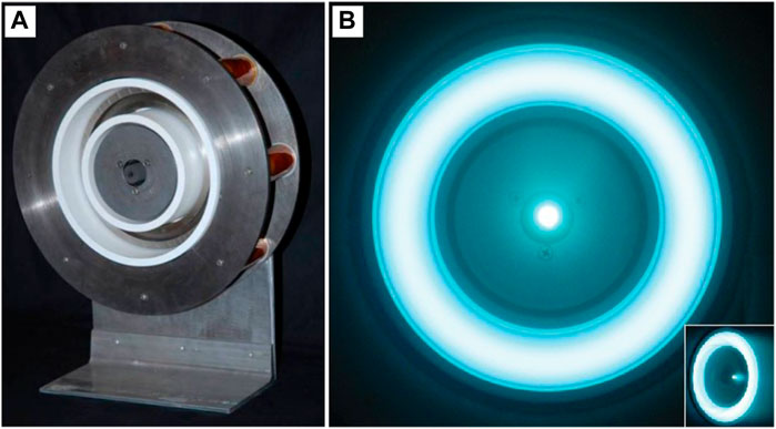
FIGURE 1. (A) The unshielded H6 Hall thruster. (B) End-on-view of the thruster and the plasma in its channel (annular ring) and the cathode (center dot). Figure reproduced here with permission from the author (Brown, 2009).

Recordings took place in the University of Michigan Plasmadynamics and Electric Propulsion Laboratory’s Large Vacuum Test Facility (LVTF) circa 2011. The LVTF is a cylindrical chamber 9 m long and 6 m in diameter and at the time was maintained at high vacuum by seven TM-1200 cryopumps with a combined pumping speed of 210,000 L/s on xenon.

A Photron SA5 FASTCAM high-speed camera placed 6.5 m axially downstream of the thruster exhaust imaged the plume through a quartz window with 152 × 192 resolution in monochrome (B&W) at a framerate of 175 kHz. The fastest mode observed was a 80 kHz cathode spoke, just below the 87.5 kHz camera Nyquist frequency. The camera used a Nikon ED AF Nikkor 80–200 mm lens at its maximum aperture of f/2.8. The bright, central cathode saturates several pixels, and the algorithms largely ignore these pixels.

In preparation for video processing, any high-speed video dataset should be thought of as a 3D matrix of pixel measurements, p(t, x, y), with dimensions of time, t, and Cartesian space, x and y, and with lengths N_t, N_x, and N_y, respectively (McDonald and Gallimore, 2013).

2.2 Video preprocessing

Before applying mode analysis algorithms, several preprocessing steps should first be considered. This section outlines two prominent steps: 1) spatial identification and normalization and 2) amplitude normalization. Other preprocessing steps, not covered here, include masking and filtering which are useful in isolating specific spatial regions or dynamics, respectively. Please note that Fourier analysis requires spatial identification as a precursor to converting to polar coordinates. The other methods discussed here are useful, but not required, for processing and analysis.

2.2.1 Spatial identification and scaling

This step identifies and the scales the spatial geometries in preparation for converting to polar coordinates, a requirement for Fourier analysis. This step is not required for POD. To identify the thruster channel origin and radius, we fit an annular Gaussian function

$\begin{array}{cc}\hfill G& \left(x,y;x_0,y_0,r_0,a,w,G_0\right)\hfill \\ \hfill & =a\text{exp}\left(-\frac{1}{2}{\left(\frac{r\left(x,y;x_0,y_0\right)-r_0}{w}\right)}^2\right)+G_0\hfill \end{array}(1)$

to the time-average, $\bar{p}(x,y)$, of the high-speed video. In this equation, r₀ is the radius of the channel, the radius at each pixel is

$r\left(x,y;x_0,y_0\right)=\sqrt{{\left(x-x_0\right)}^2+{\left(y-y_0\right)}^2},(2)$

x₀ and y₀ are the center (origin) of the channel, a is the amplitude, w is related to the channel width, and G₀ is an offset.

With these fit parameters solved, we next center and normalize the spatial coordinates to the channel radius (i.e., x_norm = (x − x₀)/r₀ and y_norm = (y − y₀)/r₀). These normalized coordinates can then be optionally multiplied by the dimensioned channel radius to provide actual units to x and y. For this work, we remain with normalized coordinates for convenience.

Figure 2 shows the results of this step as applied to the time-averaged video, $\bar{p}(x,y)$, of our H6 dataset. In this figure, the two regions with the most plasma dynamics, the annular channel and center cathode, are clearly visible. The pixel intensity has raw integer units based on the camera’s 12 bit depth. The pixels associated with the cathode’s center were allowed to saturate to better capture dynamics in the channel, and the pixels adjacent to the saturated pixels still capture the cathode’s dynamics. The channel radius, r₀, as identified by the Gaussian fit, is indicated with a black dashed line. The channel edges, indicated with white dashed lines, are identified as approximately at (r₀ ± w)/r₀. The x and y coordinates have been centered and normalized to the channel radius as described above.

FIGURE 2

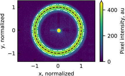
FIGURE 2. An annular Gaussian function is fit to the time-averaged video and identifies the channel origin and radius. The video’s coordinates are then centered at the origin and normalized by the channel radius.

Alternatives to the annular Gaussian fit have been used in previous Hall thruster work. McDonald (McDonald and Gallimore, 2013) discussed both the Kasa (Kåsa, 1976) and Taubin (Taubin, 1991) methods and recommended Taubin for cases where the entire channel annulus is not visible. Another option previously used (Romadanov et al., 2019) is a circle detection algorithm called a Hough transform. While no one method is obviously superior over the others, we recommend using 1) the Gaussian fit presented here because the solved parameters are directly relatable to physical dimensions or 2) the Hough transform as it is available prewritten in many programming languages.

2.2.2 Video amplitude scaling

This step scales the video’s arbitrary intensity measurements to a more meaningful range and is optional for both Fourier and POD methods. Common practice is to assume that oscillations in a video’s amplitude is roughly linear with the plasma density oscillations (Darnon et al., 1997) and that camera measurements are linear with light emission (Vora et al., 1997). As we cannot scale the data to a definitive physical value, this section instead discusses several data normalization methods to provide better physical intuition of the oscillations.

Before normalizing, the first step is to subtract the time-averaged image (also known as AC coupling) from each frame of the raw video dataset to better isolate the oscillations.

Next, we normalize the video amplitude in one of two ways: pixel-wise normalization or channel-average normalization. The first method divides each pixel by its standard deviation in time, and this has the advantage of making the mode dynamics easier to visualize after mode decomposition. Unfortunately, this method artificially amplifies the oscillations at different spatial locations and makes quantifying global mode amplitudes untenable. As an alternative, the second option divides each pixel by the average brightness within the channel, which allows the modes to be scaled as a percentage of the average channel brightness. While both methods are used in this work, channel-average normalization is default.

Figure 3 shows the results of AC coupling and channel normalization at two separate instances in time. At t = 22.9 ms (Figure 3A), the normalized video snapshot reveals a dominant 3-lobed azimuthal wave (m = 3 mode) in the channel. At t = 24.8 ms (Figure 3B), a 4-lobed azimuthal wave (m = 4 mode) is dominant. The amplitudes of both modes are around 10% of the average channel brightness. Both snapshots also show an m = 1 azimuthal wave around the cathode.

FIGURE 3

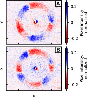
FIGURE 3. Two time snapshots, that have been AC coupled and normalized by the average channel brightness, reveal prominent mode structures. (A) At t = 22.9 ms, an m = 3 mode is dominant in the channel. (B) At t = 24.8 ms, an m = 4 mode is dominant in the channel. Both snapshots show an m = 1 mode around the cathode.

3 Fourier-based methods

Fourier based algorithms are the most established methods for mode decomposition and identification in HT high-speed video (McDonald et al., 2011; McDonald and Gallimore, 2013; Jorns and Hofer, 2014; Romadanov et al., 2019). This is because Fourier series’ bases are periodic sines and cosines and are therefore ideal for characterizing wave-like oscillations, such as plasma waves. In this section, we use Fourier analysis to characterize simultaneous m = 0 and m > 0 modes associated with the thruster discharge channel and cathode in addition to mode hopping between the m = 3 and m = 4 modes in the channel.

3.1 Detecting modes

Mode dynamics in Hall thruster plasmas are typically characterized by oscillating waves with slowly evolving amplitudes and frequencies. The easiest way to detect these modes is to apply FFT and Welch-averaged FFT (Welch, 1967) algorithms to diagnostic measurements of signal pixels of the high-speed video. Figure 4 shows an example of this applied to three signals from our dataset: the discharge current flowing from the anode to cathode, a high-speed pixel centered in the channel, and a high-speed pixel adjacent to the cathode.

FIGURE 4

FIGURE 4. Three signals are analyzed (a pixel in the thruster channel (r/r₀ = 1), a pixel adjacent to the thruster cathode (r/r₀ = 0.1), and the discharge current), and their power spectrum reveals the existence of several prominent modes (peaks). (A) The three time-series signals over 1 ms. Each has been subtracted by their mean and divided by their standard deviation. (B) Their power spectrums, calculated over 100 ms.

Figure 4A shows a 1 ms time window of the three signals and that they have similar oscillatory behavior. Each signal has been AC coupled and normalized by its standard deviation for ease of comparison.

Figure 4B shows the Welch-averaged FFT of each signal over 100 ms, and the resulting power spectrum reveals prominent frequency peaks with each. Most notable is a broad spectrum peak at 20 kHz that is common to all three signals. Additional peaks at 7.5 kHz and 80 kHz are unique to the channel and cathode measurements, respectively; this uniqueness suggests that their dynamics are isolated to their respective regions. The broader width of the 20 kHz peak suggests that its frequency is more erratic than the two narrower peaks. The remainder of this paper will identify the modes associated with these three peaks and few less pronounced peaks.

3.2 Azimuthal and radial binning

Waves around the channel and cathode of a Hall thruster are primarily azimuthal (Choueiri, 2001) with the approximate Fourier form

$p\left(t,\theta \right)\sim e^{i\left(m\theta -\omega t\right)}(3)$

where m is the integer azimuthal mode number, θ is the azimuthal angle, and ω = 2πf is the angular frequency. After scaling the video’s coordinates and amplitudes (Section 2.2), the next step is convert the 3D video, p(t, x, y), in Cartesian coordinates to a 2D video, p(t, θ), in polar coordinates so that it matches Eq. 3. To do this, we first isolate the channel region (i.e. 0.9 < r/r₀ < 1.1) with radial masking and discard the rest. The radial dependence within this narrow region is assumed constant, and the radial coordinate is therefore dropped.

Next, we convert the unmasked x and y coordinates within the channel to the azimuthal coordinate with a four-quadrant inverse tangent function, θ(x, y) = arctan2(y, x). The resulting data is azimuthally binned and averaged to provide a result with uniform azimuthal spacing.

Figure 5 illustrates the azimuthal and radial binning for a single time snapshot (t = 22.9 ms). Figure 5A shows the radial mask isolating a narrow region within the channel and also the edges of N_θ = 100 azimuthal bins; Figure 5B shows the unbinned values (black) overlayed by the bin-averaged result (red). This shows a clear m = 3 structure and also a few non-ideal features: a non-uniform spacing between peaks, a steepened waveform, and a weak fourth peak at 3π/4. This process is repeated for each time step within p(t, x, y), and the result is the 2D dataset, p(t, θ), within the channel.

FIGURE 5

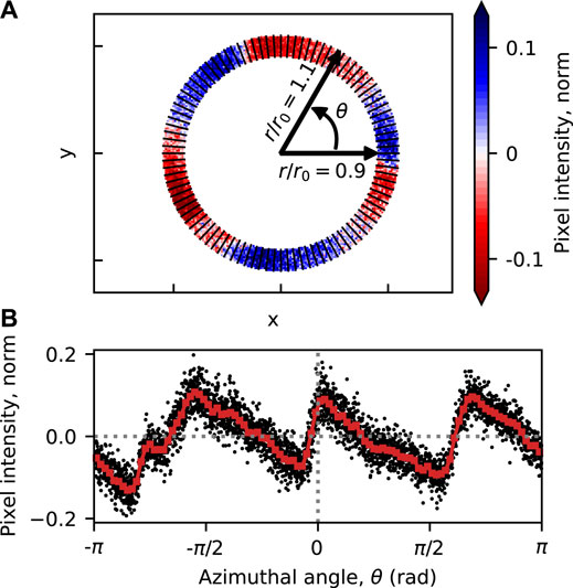
FIGURE 5. The azimuthal binning process for a single instant in time is shown. (A) A radial mask isolates a narrow radial region within the channel, and the N_θ=100 azimuthal bin boundaries are overlayed. (B) The average of each azimuthal bin (red) overlays the raw (black) data.

In this example, we applied the binning process to the channel region. However, this same procedure could be applied to other radial regions, including the region around the cathode (Jorns and Hofer, 2014) or at radial slices between the cathode and channel. Optionally, multiple radial slices could be made to provide a 3D dataset, p(t, θ, r).

3.3 Azimuthal mode identification

With p(t, θ) solved and matching the assumed Fourier form (Eq. 3), we can next identify the azimuthal modes within the channel. To do this, we apply a 2D FFT, ${\mathcal{F}}_{t,\theta }$, in both time and θ to identify the mode numbers and their characteristic frequencies. This provides the 2D complex matrix,

$P\left(\omega ,m\right){=\mathcal{F}}_{t,\theta }\left\{p\left(t,\theta \right)\right\},(4)$

with dimensions in angular frequency, ω, and azimuthal mode number, m, and with dimensional lengths, N_t and N_θ, respectively. Note that the coordinates ω = 2πf and m range between their negative and positive Nyquist frequencies (−87.5 kHz $\le f<$ 87.5 kHz and −N_θ/2 ≤ m < N_θ/2). Due to symmetry, the negative frequencies can be truncated.

The absolute value of this result, $\left|P(\omega ,m)\right|$, is the azimuthal dispersion relationship within the channel and is shown in Figure 6A. It reveals a series of evenly-spaced discrete modes (2 ≤ m ≤ 5) and what appears to be a continuous wave. Both the continuous wave and the discrete modes are propagating clockwise (negative θ) and therefore have negative wavenumbers. By convention, we present the azimuthal modes and wave numbers as positive.

FIGURE 6

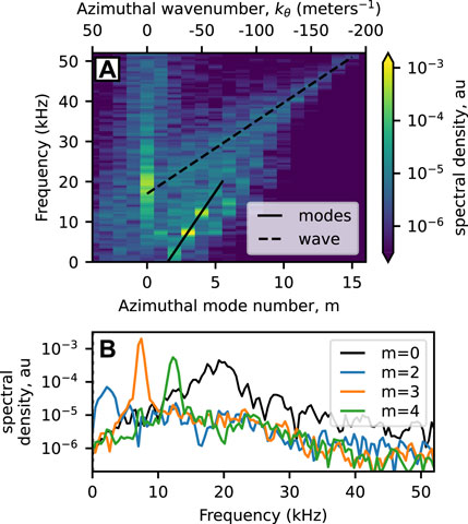
FIGURE 6. (A) The azimuthal dispersion plot within the channel (not around the cathode). A continuous wave and series of azimuthal mode numbers are identified and travel counter-clockwise (i.e., are negative). (B) The power spectrum of select mode numbers within the channel helps to identify their characteristic frequency. Please note that the frequency axes are trimmed to ≈ 50 kHz because no dynamics in the channel were present at higher frequencies.

Figure 6B shows several slices of the dispersion relationship at m = 0, 2, 3, and 4 and more clearly identifies the peaks originally observed in Figure 4B. From this plot, the m = 0 mode is the broad-spectrum peak at 20 kHz, the m = 3 mode is the narrow peak at 7.5 kHz, and the m = 4 mode is the peak at 12.5 kHz. In addition, a weak m = 2 mode is observed at 2.5 kHz. Figure 6B shows that all three of the indicated m > 0 modes have a roughly uniform spacing of 5 kHz. Figure 6A also identifies an m = 6 mode at roughly double the m = 3 frequency which makes it a harmonic of the m = 3 mode (Yamada et al., 2010). To observe the 80 kHz peak in Figure 4B, the above analysis could be applied to the region around the cathode instead of inside the channel.

3.4 Mode evolution

To capture the time evolution of each mode, we apply 1D FFT, ${\mathcal{F}}_{\theta }$, to each time step in the 2D dataset, p(t, θ), along the θ dimension. The result is the 2D complex matrix,

$P\left(t,m\right){=\mathcal{F}}_{\theta }\left\{p\left(t,\theta \right)\right\}(5)$

with dimensions in time, t, and azimuthal mode number, m. Depending on the FFT algorithm, p(t, m) then needs to be multiplied by a constant to return the correct amplitude, typically 2/N_θ. Figure 7 plots the real (cosine) component, the imaginary (sine) component, and the amplitude of p(t, m) at m = 0, 3, and 4 and shows the time evolution of each. Figure 7A reveals the m = 0 breathing mode to have a mostly consistent amplitude around 10%–20% of the average channel brightness. Figures 7B, C shows the m = 3 and m = 4 modes, respectively, with amplitudes between 3% and 5%. These figures also clearly identify repeated mode hopping between these two modes. In the m = 3 and 4 figures, the real component leads the real component by roughly 90°, indicating that the modes are rotating clockwise. The m = 0 mode is not rotating, and therefore its imaginary component is zero.

FIGURE 7

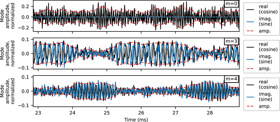
FIGURE 7. Time evolution of the m = 0, 3 and 4 modes as captured by the 1D FFT in θ. Repeated mode hopping is observed between the m = 3 and m = 4 modes. The signals are normalized by the average channel brightness.

3.5 The modes’ spatial structures

To isolate the spatial structure associated with each mode, we first apply 1D Fourier analysis,

$P\left(f,x,y\right){=\mathcal{F}}_t\left\{p\left(t,x,y\right)\right\},(6)$

to each pixel in the 3D video, p(t, x, y), with respect to time. Next, we index the resulting matrix, p(f, x, y), at the frequencies associated with each mode as identified in Figure 6. Figure 8 shows the resulting real (cosine) and imaginary (sine) component of each mode, which reveals the spatial extent and phase of each. The number of peaks and troughs of each structure accurately corresponds to its mode number. This approach is a computationally efficient alternative to bandpass-filtering each pixel as done previously (McDonald and Gallimore, 2013). These plots are also nearly identical to plots in previous works (Jorns and Hofer, 2014; Baird, 2020) with the difference being that the past works plot the phase, atan (imag./real), of each mode instead of the real and imaginary components.

FIGURE 8

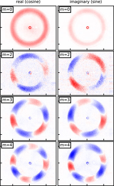
FIGURE 8. Fourier analysis (Eq. 6) reveals the spatial structure of several dominant modes in the channel. The amplitude is spectral density (au) with each subfigure having a different scaling.

For better visualization, each pixel in p(t, x, y) can optionally be normalized by its standard deviation before applying Eq. 6. Figure 9 shows an example of this for the m = 3 mode. This figure reveals improved spatial detail within the channel and also suggests mode structure outside the channel as well.

FIGURE 9

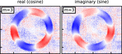
FIGURE 9. Pre-normalizing each pixel in p (t, x, y) by its standard deviation instead of by the average channel brightness provides better visualization of the mode structure. Amplitude is spectral density (au). These plots are directly comparable to the m = 3 subplots in Figure 8 where the channel normalization is used.

3.6 Fourier methods conclusion

In this section, we applied the Fourier mode decomposition and identification methods to our H6 high-speed video dataset. First, the FFT of individual pixels was able to identify the presence of coherent mode dynamics in the channel and cathode regions. After radially and azimuthally binning the data within the channel, a 2D FFT provided an azimuthal dispersion plot and helped relate mode numbers to their characteristic frequency. A 1D FFT was then used to isolate the temporal evolution of each mode and most notably identified mode hopping between the m = 3 and m = 4 modes in the channel. Finally, a 1D FFT was applied to the original video, and plotting the frequencies associated with each provided the mode’s spatial structure. While these methods were only applied to the channel region in this work, this process can be applied to any radial region including around the cathode.

4 SVD-based methods

Matrix factorization-based methods, based on the SVD (Singular Value Decomposition) algorithm (Golub and Reinsch, 1970), are an alternative approach to decomposing and identifying modes from high-speed video and provide several advantages over Fourier methods. Below, we first detail the SVD algorithm, discuss the simplest SVD-based mode analysis method (the POD algorithm), and apply it to the present dataset.

4.1 The SVD algorithm

The SVD algorithm is the foundation for POD and for more advanced algorithms. This section discusses the SVD algorithm and its implementation.

The most notable feature of SVD is that it does not presume spatial or temporal bases (e.g., Fourier sines and cosines) when decomposing coherent structures. Instead, SVD provides a tailored, orthonormal basis for a particular video dataset by minimizing the L₂ norm (error) between the original video and the video reconstructed from the new SVD bases (Brunton and Kutz, 2019). SVD also orders each basis from the highest to lowest contribution (amplitude) so that the strongest coherent structure appears first, then the second strongest, etc. In contrast, Fourier orders its bases by increasing frequency or wavenumber. A downside to SVD’s ordering is that post-processing (either visually or algorithmically) is often required to associate each identified SVD structure with its Fourier counterpart. Examples of this are provided later in this paper. An advantage of SVD is that it does not require any preprocessing, most notably conversion to a particular coordinate system (e.g., converting the Cartesian video to polar). More details on the SVD algorithm can be found in the extensive literature on the subject (Golub and Reinsch, 1970; Golub and Loan, 1996; Woolfe et al., 2008; Brunton and Kutz, 2019).

In order to apply the SVD algorithm to a video dataset, p(t, x, y), we first convert it from 3D to 2D. We do this by stacking the data associated with the two spatial dimensions into a single spatial dimension, z = stack(x, y) to get the 2D p(t, z) dataset with dimensions in time and space and with sizes N_t and N_z = N_xN_y, respectively. This process is the 3D equivalent of stacking columns in a 2D matrix to get a 1D array. The Python data structure xarray has built-in functions (stack and unstack) that make stacking and unstacking very convenient. By convention, we also transpose p(t, z) to p(z, t) so that the spatial dimension is ordered before the temporal dimension. For our high-speed video dataset, N_z > N_t, so p (z, t) is a “tall-skinny” matrix.

When applied to p(z, t), the SVD algorithm outputs three real matrices: U(z, n), Σ(n, n), and V(t,n)^T. Here, we are using n to represent the SVD basis numbers to distinguish them from the Fourier mode numbers, m. First, U(z, n) is a non-square, 2D matrix associated with the spatial bases (called the topos, i.e., “shapes”) with dimensions of space, z, and mode number, n, and lengths N_z and N_n = N_t, respectively. Σ(n, n) is a square 2D diagonal matrix associated with the basis energies (these diagonal values are referred to as the singular values) with dimensions n by n each with length N_n. Finally, the transposed matrix, V(t,n)^T, is a square 2D matrix that contains the temporal evolution of the bases (called the chronos, i.e., “times”) with dimensions of n and t, each with length, N_n = N_t. For example, many SVD algorithms return Σ(n, n) as 1D array of its diagonal elements.

Multiplying these three matrices together,

$\begin{array}{cc}\hfill & U\left(z,n\right)\mathrm{\Sigma }\left(n,n\right)V{\left(t,n\right)}^T\hfill \\ \hfill & =\left[\begin{array}{cccc}\hfill |\hfill & \hfill |\hfill & \hfill \hfill & \hfill |\hfill \\ \hfill u_1\hfill & \hfill u_2\hfill & \hfill \dots \hfill & \hfill u_N\hfill \\ \hfill |\hfill & \hfill |\hfill & \hfill \hfill & \hfill |\hfill \end{array}\right]\left[\begin{array}{ccc}\hfill {\sigma }_1\hfill & \hfill \hfill & \hfill \hfill \\ \hfill \hfill & \hfill \ddots \hfill & \hfill \hfill \\ \hfill \hfill & \hfill \hfill & \hfill {\sigma }_N\hfill \end{array}\right]{\left[\begin{array}{cccc}\hfill |\hfill & \hfill |\hfill & \hfill \hfill & \hfill |\hfill \\ \hfill v_1\hfill & \hfill v_2\hfill & \hfill \dots \hfill & \hfill v_N\hfill \\ \hfill |\hfill & \hfill |\hfill & \hfill \hfill & \hfill |\hfill \end{array}\right]}^T\hfill \\ \hfill & ={\sigma }_1{u}_1{v}_1^T+{\sigma }_2{u}_2{v}_2^T+\cdots +{\sigma }_N{u}_N{v}_N^T\hfill \\ \hfill & \approx p\left(z,t\right),\hfill \end{array}(7)$

reconstructs p(z, t) with remarkable accuracy, owing to the orthonormality of the u_n and v_n and the ordering of bases from strongest to weakest. Related to this, another major advantage of SVD over Fourier is its ability to reconstruct data (like this high-speed video) with fewer bases. In this equation, u_n, σ_n, and v_n, are the topo, singular value (energy), and chrono associated with the nth basis, which are ordered from highest contribution (energy) to lowest. In Eq. 7, the multiplication of $u_n{v}_n^T$ is an outer product. As a final note, we refer to σ_n as the energy because our measurement is light intensity. However, it is common in the literature to measure the velocity or magnetic field and therefore refer to ${\sigma }_n^2$ as the energy.

4.2 Proper orthogonal decomposition (POD)

The POD method, also referred to as Biorthogonal Decomposition (BD), has been used extensively for plasma physics datasets (Dudok de Wit et al., 1994) but has only been very recently introduced to Hall thruster and hollow cathode high-speed video (Désangles et al., 2020; Becatti et al., 2021). The POD algorithm is nearly identical to the SVD algorithm with the main distinction being that the U, Σ, and V^T matrices are often trimmed to retain a smaller set of bases (e.g., n < 30).

After applying the POD algorithm (Section 4.1) to our dataset, we inspect each of the U, Σ, and V^T matrices to identify and interpret the dynamics associated with each mode. First, the energy for each basis, σ_n, is plotted in Figure 10. This highlights that the lower numbered bases capture the majority of the dynamics of the video and are therefore the focus of this section.

FIGURE 10

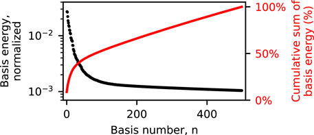
FIGURE 10. The SVD algorithm orders its bases from highest to lowest energy (i.e., their total contribution to the reconstructed video), and therefore the lower numbered bases are more likely to contain the most prominent dynamics.

To visualize the spatial bases (topos), we unstack the z dimension in U(z, n) to get U(x, y, n). Figure 11 shows the first 10 topos, u_n, and each reveals an m = 0 or m > 0 azimuthal structure in the channel or around the cathode. The bases associated with m > 0 rotating modes each have a near-duplicate (but rotated) topo that represents an effective sine-cosine pairing. For example, the n = 2 and 3 bases are effectively the Fourier sine and cosine (real and imaginary) components of the m = 3 rotating mode in the channel and therefore well matches the modes in Figure 8. Note that the POD bases associated with the m = 2 Fourier mode is not shown in Figure 11 despite being present (as shown by Figure 8). This is because its energy contribution is lower than the first 10 POD bases.

FIGURE 11

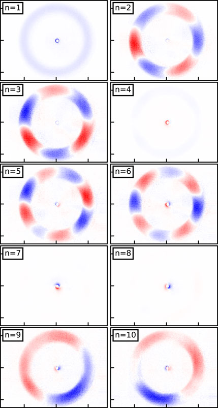
FIGURE 11. The POD topos for the first 10 bases show m = 0 or m > 0 azimuthal structures in the channel or around the cathode. Amplitude units are arbitrary. By inspection, topos correspond to Fourier sine/cosine pairs as shown in Table 1.

Each of these topos has an associated time evolution, i.e., chronos, associated with it. Several select chronos, ${\sigma }_n{v}_n^T$, are plotted in Figure 12. Referring back to Figure 11, we see that their corresponding topos are roughly equivalent to the m = 0, 3, and 4 Fourier modes in the channel. Therefore, it is not a surprise that their chronos in Figure 12 are nearly identical to the Fourier-solved mode evolution shown in Figure 7.

FIGURE 12

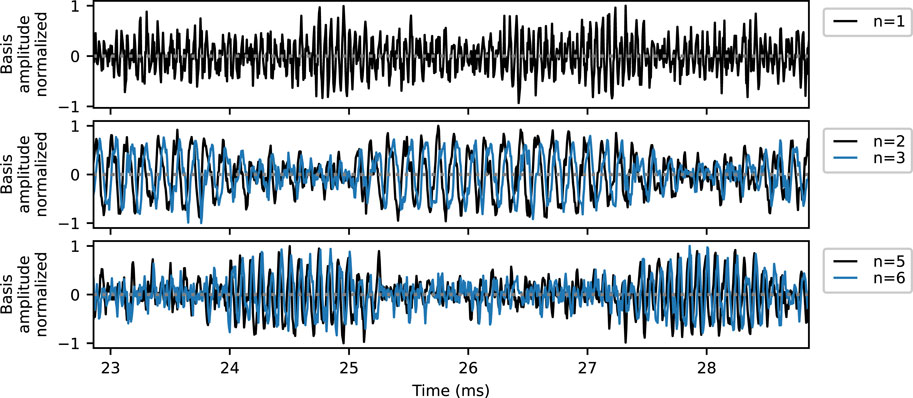
FIGURE 12. The POD chronos for the n = 1, 2, 3, 5 and 6 bases. These bases are roughly equivalent to the time evolutions of the m = 0, 3, and 4 Fourier modes in Figure 7.

Finally, the Welch-averaged FFT of select POD chronos are shown in Figure 13. Note that only a single basis from a sine-cosine pair is presented as their power spectrums of each are nearly identical. Many of the peaks in Figure 13 are the same peaks as identified in the raw data (Figure 4B) and the Fourier mode analysis (Figure 6B). A new structure is revealed by the n = 4 basis, related to the Fourier m = 1 cathode mode, which has two peaks around 38 and 80 kHz. From this analysis alone, it is not clear if the m = 1 cathode mode truly has two characteristic frequencies, if this basis is the combination of two Fourier modes, or if there is another explanation.

FIGURE 13

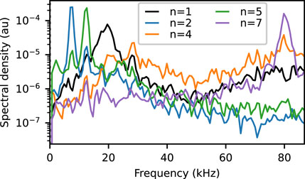
FIGURE 13. The Welch-averaged FFT of select POD chronos helps in identifying the presence of a coherent mode structure and their characteristic frequencies. This figure is directly comparable to the Fourier results in Figure 6B with the exception that this figures includes dynamics from both the anode and cathode regions and Figure 6B only contains dynamics within the channel (and therefore no notable signal at 80 kHz).

Comparing the results of the POD bases (Figures 11–13) to the Fourier modes (Figures 6–8) reveals a near one-to-one mapping as is indicated in Table 1. This is not too surprising as there are already established scenarios in which POD modes reduce to Fourier modes (Holmes et al., 2012).

TABLE 1

TABLE 1. The POD bases and Fourier modes show a near one-to-one mapping.

4.3 SVD methods conclusion

The primary advantage of the SVD-based methods is that they do not presume a universal basis, Fourier or otherwise, and instead create tailored bases which optimally capture particular features of the dynamics. In addition, these methods require less preconditioning of the video, e.g., radial binning and converting the pixel coordinates to polar, and therefore they can provide detailed images of the spatial structures of each basis or mode (Figure 11). The most basic SVD method, POD, is easier to implement than the Fourier methods, does not require a linear assumption, and produces very similar results. More advanced SVD methods, such as DMD, have potential for Hall thruster modal analysis but require more development.

5 Conclusion

This work provided a survey of existing Fourier and new SVD-based mode decomposition techniques for high-speed Hall thruster video data. To highlight the implementation of these methods, they were each applied to the same H6 dataset which contained simultaneous modes associated with the channel and cathode. Both Fourier and POD methods were able to characterize the spatial and temporal evolution of each mode, including mode hopping between the m = 3 and m = 4 channel modes. Both methods also had their various strengths and weaknesses.

Fourier methods are well suited for characterizing linear wave dynamics and therefore excel at identifying both discrete mode and continuous wave dynamics in the various regions of the Hall thruster plasma. A notable feature of the Fourier methods are their ability to naturally provide dispersion relationships. However, Fourier methods require preprocessing, e.g., converting the video to polar coordinates, which adds computational complexity.

POD, an alternative to Fourier, does not introduce new physical information; instead it represents the dynamics in an alternative format that provides several advantages. The first advantage is that POD produces a tailored set of orthogonal bases for each dataset that are ordered by their relative amplitudes (high to low), and these bases do not presume any form (e.g., sines and cosines in Fourier). Second, the POD method is relatively simple to implement as preprocessing, most notably coordinate conversion, is optional. Third, POD can naturally identify mode structures and their associated spatial locations and can therefore be more easily combined with techniques such as bicoherence analysis to study coupling between dynamics (Brooks et al., 2022).

Together, Fourier and POD methods provide for a more complete toolkit for studying global Hall thruster dynamics as captured by high-speed imaging. Moving forward, we recommend first applying POD to a dataset in order to identify its major dynamics and the spatial locations of each. With this information, Fourier methods can then be intelligently targeted to extract dispersion relationships or other select modal information. The code and data used in this work are made are available online (Brooks, 2021) to assist future researchers.

Data availability statement

The datasets presented in this study can be found in online repositories. The names of the repository/repositories and accession number(s) can be found in the article/Supplementary material.

Author contributions

JB is the primary author and carried out the most of the research and writing. AK contributed significantly to the POD section in terms of research and writing. MM provided guidance and helped with much of the Fourier algorithms and interpretation of the results. All authors contributed to the article and approved the submitted version.

Funding

This analysis was performed while JB held an NRC Research Associateship award at the Naval Research Laboratory (NRL), with JB and MM supported by the NRL Base Program. The imaging data was collected at the University of Michigan by MM under advisor Alec Gallimore in the Plasmadynamics and Electric Propulsion Laboratory, where the use of the Photron SA5 FASTCAM was made possible via grant FA9550-09-1-0695 from the Air Force of Scientific Research (AFOSR). AK acknowledges funding from the Army Research Office (ARO W911NF-19-1-0045) and the Air Force Office of Scientific Research (AFOSR FA9550-18-1-0200).

Conflict of interest

The authors declare that the research was conducted in the absence of any commercial or financial relationships that could be construed as a potential conflict of interest.

Publisher’s note

All claims expressed in this article are solely those of the authors and do not necessarily represent those of their affiliated organizations, or those of the publisher, the editors and the reviewers. Any product that may be evaluated in this article, or claim that may be made by its manufacturer, is not guaranteed or endorsed by the publisher.

References

Baird, M. (2020). Investigating newly discovered oscillation modes in magnetically shielded Hall effect thrusters utilizing high speed diagnostics. Kalamazoo, MI: Ph.D. thesis, Western Michigan University.

Google Scholar

Becatti, G., Goebel, D. M., and Zuin, M. (2021). Observation of rotating magnetohydrodynamic modes in the plume of a high-current hollow cathode. J. Appl. Phys. 129, 033304. doi:10.1063/5.0028566

CrossRef Full Text | Google Scholar

Benner, P., Gugercin, S., and Willcox, K. (2015). A survey of projection-based model reduction methods for parametric dynamical systems. SIAM Rev. 57, 483–531. doi:10.1137/130932715

CrossRef Full Text | Google Scholar

Boeuf, J.-P. (2017). Tutorial: Physics and modeling of Hall thrusters. J. Appl. Phys. 121, 011101. doi:10.1063/1.4972269

CrossRef Full Text | Google Scholar

Brooks, J. (2021). Code and data for a comparison of fourier and pod mode decomposition methods for high-speed hall thruster video.

Google Scholar

Brooks, J., Georgin, M., and McDonald, M. (2022). “Identification of mode dynamics and mode coupling in a multi-orifice hollow cathode plume,” in 37th international electric propulsion conference (Cambridge, Massachusetts). IEPC 2022-150.

Google Scholar

Brown, D. L. (2009). Investigation of low discharge voltage Hall thruster characteristics and evaluation of loss mechanisms. PhD thesis, University of Michigan.

Google Scholar

Brunton, S. L., and Kutz, J. N. (2019). Data-driven science and engineering: Machine learning, dynamical systems, and control 1st ed. Cambridge: Cambridge University Press.

Google Scholar

Choueiri, E. Y. (2001). Plasma oscillations in Hall thrusters. Phys. Plasmas 8, 1411–1426. doi:10.1063/1.1354644

CrossRef Full Text | Google Scholar

Dale, E. (2019). “Two-zone hall thruster breathing mode mechanism, part I: Theory,” in 36th international electric propulsion conference.

Google Scholar

Darnon, F., Lyszyk, M., Bouchoule, A., Darnon, F., Lyszyk, M., and Bouchoule, A. (1997). “Optical investigation on plasma investigations of SPT thrusters,” in 33rd joint propulsion conference and exhibit (American Institute of Aeronautics and Astronautics).

CrossRef Full Text | Google Scholar

Désangles, V., Shcherbanev, S., Charoy, T., Clément, N., Deltel, C., Richard, P., et al. (2020). Fast camera analysis of plasma instabilities in Hall effect thrusters using a POD method under different operating regimes. Atmosphere 11, 518. doi:10.3390/atmos11050518

CrossRef Full Text | Google Scholar

Dudok de Wit, T., Pecquet, A., Vallet, J., and Lima, R. (1994). The biorthogonal decomposition as a tool for investigating fluctuations in plasmas. Phys. Plasmas 1, 3288–3300. doi:10.1063/1.870481

CrossRef Full Text | Google Scholar

Florenz, R., Liu, T., Gallimore, A., Kamhawi, H., Brown, D., Hofer, R., et al. (2012). “Electric propulsion of a different class: The challenges of testing for MegaWatt missions,” in 48th AIAA/ASME/SAE/ASEE joint propulsion conference & exhibit, joint propulsion conferences (AIAA).

CrossRef Full Text | Google Scholar

Georgin, M. P., Jorns, B. A., and Gallimore, A. D. (2019). Correlation of ion acoustic turbulence with self-organization in a low-temperature plasma. Phys. Plasmas 26, 082308. doi:10.1063/1.5111552

CrossRef Full Text | Google Scholar

Goebel, D. M., Jameson, K. K., Katz, I., and Mikellides, I. G. (2007). Potential fluctuations and energetic ion production in hollow cathode discharges. Phys. Plasmas 14, 103508. doi:10.1063/1.2784460

CrossRef Full Text | Google Scholar

Goebel, D. M., and Katz, I. (2008). “Fundamentals of electric propulsion: Ion and Hall thrusters,” in JPL space science and Technology series No. 1 (NASA JPL.

Google Scholar

Golub, G. H., and Loan, C. F. V. (1996). Matrix computations 3rd ed. Baltimore: Johns Hopkins University Press.

Google Scholar

Golub, G. H., and Reinsch, C. (1970). Singular value decomposition and least squares solutions. Numer. Math. 14, 403–420. doi:10.1007/bf02163027

CrossRef Full Text | Google Scholar

Hall, S., Jorns, B., Gallimore, A., Kamhawi, H., Haag, T., Mackey, J., et al. (2017). “High-power performance of a 100-kW class nested hall thruster,” in 35th international electric propulsion conference.

Google Scholar

Hansen, C., Victor, B., Morgan, K., Jarboe, T., Hossack, A., Marklin, G., et al. (2015). Numerical studies and metric development for validation of magnetohydrodynamic models on the HIT-SI experimenta). Phys. Plasmas 22, 056105. doi:10.1063/1.4919277

CrossRef Full Text | Google Scholar

Hara, K., Sekerak, M. J., Boyd, I. D., and Gallimore, A. D. (2014). Mode transition of a Hall thruster discharge plasma. J. Appl. Phys. 115, 203304. doi:10.1063/1.4879896

CrossRef Full Text | Google Scholar

Holmes, P., Lumley, J. L., Berkooz, G., and Rowley, C. W. (2012). Turbulence, coherent structures, dynamical systems and symmetry. Cambridge University Press.

Google Scholar

Janes, G. S., and Lowder, R. S. (1966). Anomalous electron diffusion and ion acceleration in a low-density plasma. Phys. Fluids 9, 1115–1123. doi:10.1063/1.1761810

CrossRef Full Text | Google Scholar

Jorns, B. A., Cusson, S. E., Brown, Z., and Dale, E. (2020). Non-classical electron transport in the cathode plume of a Hall effect thruster. Phys. Plasmas 27, 022311. doi:10.1063/1.5130680

CrossRef Full Text | Google Scholar

Jorns, B. A., and Hofer, R. R. (2014). Plasma oscillations in a 6-kW magnetically shielded Hall thruster. Phys. Plasmas 21, 053512. doi:10.1063/1.4879819

CrossRef Full Text | Google Scholar

Kaptanoglu, A. A., Morgan, K. D., Hansen, C. J., and Brunton, S. L. (2020). Characterizing magnetized plasmas with dynamic mode decomposition. Phys. Plasmas 27, 032108. doi:10.1063/1.5138932

CrossRef Full Text | Google Scholar

Kaptanoglu, A. A., Morgan, K. D., Hansen, C. J., and Brunton, S. L. (2021). Physics-constrained, low-dimensional models for magnetohydrodynamics: First-principles and data-driven approaches. Phys. Rev. E 104, 015206. doi:10.1103/physreve.104.015206

PubMed Abstract | CrossRef Full Text | Google Scholar

Kåsa, I. (1976). “A circle fitting procedure and its error analysis,” in IEEE transactions on instrumentation and measurement IM-25, 8–14.

Google Scholar

Levesque, J. P., Rath, N., Shiraki, D., Angelini, S., Bialek, J., Byrne, P. J., et al. (2013). Multimode observations and 3D magnetic control of the boundary of a tokamak plasma. Nucl. Fusion 53, 073037. doi:10.1088/0029-5515/53/7/073037

CrossRef Full Text | Google Scholar

McDonald, M., Bellant, C., Pierre, B. St., and Gallimore, A. (2011). “Measurement of cross-field electron current in a hall thruster due to rotating spoke instabilities,” in 47th AIAA joint prop. Conf.

CrossRef Full Text | Google Scholar

McDonald, M., and Gallimore, A. (2011c). “Parametric investigation of the rotating spoke instability in hall thrusters,” in 32nd international electric propulsion conference (IEPC 2011-242 (Wiesbaden, Germany.

Google Scholar

McDonald, M. S., and Gallimore, A. D. (2013). “Comparison of breathing and spoke mode strength in the H6 Hall thruster using high speed imaging,” in 33rd international electric propulsion conference (Washington, DC.

Google Scholar

McDonald, M. S., and Gallimore, A. D. (2011a). “Measurement of cross-field electron current in a Hall thruster due to rotating spoke instabilities,” in 47th AIAA/ASME/SAE/ASEE joint propulsion conference & exhibit. (AIAA 2011-5810, 2011).

CrossRef Full Text | Google Scholar

McDonald, M. S., and Gallimore, A. D. (2011b). Rotating spoke instabilities in hall thrusters. IEEE Trans. Plasma Sci. 39, 2952–2953. doi:10.1109/tps.2011.2161343

CrossRef Full Text | Google Scholar

Noack, B. R., Afanasiev, K., Morzyński, M., Tadmor, G., and Thiele, F. (2003). A hierarchy of low-dimensional models for the transient and post-transient cylinder wake. J. Fluid Mech. 497, 335–363. doi:10.1017/s0022112003006694

CrossRef Full Text | Google Scholar

Oudheusden, B., Scarano, F., Van Hinsberg, N., and Watt, D. (2005). Phase-resolved characterization of vortex shedding in the near wake of a square-section cylinder at incidence. Exp. Fluids 39, 86–98. doi:10.1007/s00348-005-0985-5

CrossRef Full Text | Google Scholar

Parker, J. B., Raitses, Y., and Fisch, N. J. (2010). Transition in electron transport in a cylindrical Hall thruster. Appl. Phys. Lett. 97, 091501. doi:10.1063/1.3486164

CrossRef Full Text | Google Scholar

Romadanov, I., Raitses, Y., and Smolyakov, A. (2019). Control of coherent structures via external drive of the breathing mode. Plasma Phys. Rep. 45, 134–146. doi:10.1134/s1063780x19020156

CrossRef Full Text | Google Scholar

Sasaki, M., Kawachi, Y., Dendy, R. O., Arakawa, H., Kasuya, N., Kin, F., et al. (2019). Using dynamical mode decomposition to extract the limit cycle dynamics of modulated turbulence in a plasma simulation. Plasma Phys. Control. Fusion 61, 112001. doi:10.1088/1361-6587/ab471b

CrossRef Full Text | Google Scholar

Schmid, P. J. (2010). Dynamic mode decomposition of numerical and experimental data. J. Fluid Mech. 656, 5–28. doi:10.1017/s0022112010001217

CrossRef Full Text | Google Scholar

Sekerak, M. J., Gallimore, A. D., Brown, D. L., Hofer, R. R., and Polk, J. E. (2016). Mode transitions in hall-effect thrusters induced by variable magnetic field strength. J. Propuls. Power 32, 903–917. doi:10.2514/1.b35709

CrossRef Full Text | Google Scholar

Taira, K., Brunton, S. L., Dawson, S., Rowley, C. W., Colonius, T., McKeon, B. J., et al. (2017). Modal analysis of fluid flows: An overview. AIAA J. 55, 4013–4041. doi:10.2514/1.j056060

CrossRef Full Text | Google Scholar

Taubin, G. (1991). “Estimation of planar curves, surfaces, and nonplanar space curves defined by implicit equations with applications to edge and range image segmentation,” in IEEE transactions on pattern analysis and machine intelligence 13. doi:10.1109/34.103273

CrossRef Full Text | Google Scholar

Taylor, R., Kutz, J. N., Morgan, K., and Nelson, B. A. (2018). Dynamic mode decomposition for plasma diagnostics and validation. Rev. Sci. Instrum. 89, 053501. doi:10.1063/1.5027419

PubMed Abstract | CrossRef Full Text | Google Scholar

Tu, J. H., Rowley, C. W., Luchtenburg, D. M., Brunton, S. L., and Kutz, J. N. (2014). On dynamic mode decomposition: Theory and applications. J. Comput. Dyn. 1, 391–421. doi:10.3934/jcd.2014.1.391

CrossRef Full Text | Google Scholar

van Milligen, B. P., Sánchez, E., Alonso, A., Pedrosa, M. A., Hidalgo, C., de Aguilera, A. M., et al. (2014). The use of the biorthogonal decomposition for the identification of zonal flows at TJ-II. Plasma Phys. Control. Fusion 57, 025005. doi:10.1088/0741-3335/57/2/025005

CrossRef Full Text | Google Scholar

Vora, P. L., Farrell, J. E., Tietz, J. D., and Brainard, D. H. (1997). “Linear models for digital cameras,” in Proceedings, IS&T’s 50th annual conference, 377–382.

Google Scholar

Welch, P. (1967). The use of fast fourier transform for the estimation of power spectra: A method based on time averaging over short, modified periodograms. IEEE Trans. Audio Electroacoustics 15, 70–73. doi:10.1109/TAU.1967.1161901

CrossRef Full Text | Google Scholar

Woolfe, F., Liberty, E., Rokhlin, V., and Tygert, M. (2008). A fast randomized algorithm for the approximation of matrices. Appl. Comput. Harmon. Analysis 25, 335–366. doi:10.1016/j.acha.2007.12.002

CrossRef Full Text | Google Scholar

Yamada, T., Itoh, S.-I., Inagaki, S., Nagashima, Y., Shinohara, S., Kasuya, N., et al. (2010). Two-dimensional bispectral analysis of drift wave turbulence in a cylindrical plasma. Phys. Plasmas 17, 052313. doi:10.1063/1.3429674

CrossRef Full Text | Google Scholar