Micro-nozzle flow and thrust prediction with high-density ratio using DSMC selection limiter

Introduction: A Direct Simulation Monte Carlo (DSMC) solver with a modified collisional routine is used to investigate an argon gas flow through a millimeter-scaled thruster nozzle with high-density ratios.

Method: The limiter scheme, denoted as the constant selection limiter (CSL), limits the possible number of selected collisional pairs to a constant value in accordance with the present simulation particles in the cell.

Results: Results of the CSL scheme are compared with the experimental and numerical results of a compressible Navier–Stokes solver and discussed in comparison with baseline DSMC simulations. The influence of collision limitation by the CSL is discussed on the stagnation pressure of the thruster and on thrust and specific impulse prediction. The application of the limiter scheme makes the prediction of stagnation pressure challenging in some cases.

Discussion: In contrast, thrust and specific impulse are predicted well, and their study remains valid. Investigated mass flow rates are 0.178 mg/s $\le \dot{m}\le$ 71.360 mg/s, and flow Knudsen numbers below Kn = 0.01 and over Kn = 10 are present. Near atmospheric conditions are reached inside the thruster, generating pressure ratios up to 3,741 along the nozzle. The computational performance of the scheme is also discussed, and speed-up factors up to 0.51 are achieved.

1 Introduction

The direct simulation Monte Carlo (DSMC) method has been used to simulate rarefied flow fields in all kinds of geometries, for example, re-entering space capsules (Shang and Chen, 2013) or nozzle geometries (Zelesnik et al., 1994) and micro-electro-mechanical systems (MEMS) (Alexeenko et al., 2002; Titov et al., 2005a; Titov et al., 2005b; Roohi et al., 2009). The method, invented and described in its original form by Bird (1994), has proven to solve flow problems correctly, where the continuum approaches break down due to the strong effects of flow rarefaction. The DSMC approach has become a standard tool in solving micro-nozzle flow problems with high Knudsen numbers because it can handle the effects of viscous boundary layers, strongly affecting the flow itself due to the large ratio of nozzle wall area to the core volume of the flow (Gomez and Groll, 2016). The method is also used to correctly analyze thruster plume behavior beyond the nozzle’s exit (Ketsdever et al., 2005) and evaluate thrust at the nozzle exit plane.

In recent years, attempts have been made to extend simulation techniques to the whole range of flow regimes and Knudsen numbers. A way to extend the numerical capabilities is to use a hybrid approach by coupling two or more numerical methods best suited for each flow regime. For example, in nozzle flows, the high-density portion of the flow may be solved using a continuum-based method, defining a zone where the first method breaks down and transferring flow quantities to a kinetic approach to solve the rarefied part of the flow. Several different hybrid approaches are described in the literature, whereat in many approaches, the DSMC method is used to solve the rarefied portion of the flow. A coupling of Navier–Stokes and DSMC solvers has successfully been applied in the past (Ivanov et al., 1997; Wang et al., 2003). Despite the high efficiency of the continuum model at low Knudsen numbers, the transfer and interpolation of flow quantities to the kinetic method are challenging using this approach. Coupling can also be achieved by combining the DSMC method with another kinetic-based method, such as a BGK (Bhatnagar-Gross-Krook model) particle model (Macrossan, 2001; Kolobov et al., 2007). Here, the coupling is more straightforward but with the cost of computational speed because BGK particle models may have requirements for the cell size and time step similar to the DSMC method. A recent development that overcomes these strict requirements is the hybrid Fokker–Planck-DSMC algorithm, which was also successfully applied to nozzle flow test cases (Gorji and Jenny, 2015). A further example of a hybrid approach is the low diffusion particle method (Burt and Boyd, 2008; Burt and Boyd, 2009), which mainly replaces the collisional routines of the DSMC and can be seen as a quasi-hybrid.

The modification of the DSMC algorithm in a more direct way to raise the computational performance is an attractive idea. As only one single approach is used to solve the whole flow field, no transfer and interpolation of flow properties has to be done, and potential sources of error can be prevented. The DSMC method naturally yields the potential to solve a flow spanning over the whole range of flow regimes because the collisional term of the Boltzmann equation is solved directly, and sampling of macroscopic quantities is done in a statistical manner. Unfortunately, the DSMC method becomes numerically very expensive near or in the continuum regime when Knudsen numbers are low due to the huge number of collisions that have to be calculated (Busse et al., 2021; Kühn and Groll, 2021; Yu et al., 2023). According to Titov and Levin (2007) and Sharma and Long (2004), collisional computing time can take up to 60% of the overall computing time, depending on the method used (Muraviev et al., 2021). In order to reduce these costs, a common approach is to limit the number of possible collisions n_c in a cell to a constant value per time step by n_c = χ N, where χ is referred to as a limiter value and N is the number of test particles in the cell. The approach is valid as in the continuum regime, velocity relaxation to the equilibrium distribution is reached after a certain number of collisions, and further collisions would not change the distribution anymore.

The literature proposes several values for the limiter χ. For example, Sharma and Long (2004) used a value of χ = 0.75 to obtain results of blast impacts on building structures. However, this value was too low for certain problems, as Titov et al. (2005a)pointed out. With an applied value of χ = 0.75, large deviations occurred in the Maxwellian distribution of test particle velocities up to approximately 50%, especially in the throat region, where density, flow velocity, and temperature rapidly changed (Titov et al., 2005a). Titov and Levin (2007) used values of χ = 0.75 and χ = 2 for the limiter to extend the DSMC method to high-pressure MEMS nozzle flows. The combination of their proposed eDSMC method and the standard DSMC yielded good results for the investigated nozzle geometry for a value of χ = 2. Bartel et al. (1994)conducted another study with a limiter value of χ = 5.

A different technique to raise the computational performance of collision calculation, which has been denoted as a selection limiter, was reported by Zhang et al. (2008). The selection limiting procedure intervenes in the selection number calculation of the applied no-time-counter (NTC) scheme by multiplying the number of selected pairs n_SP with a function S dependent on gradient length local Knudsen numbers Kn_GLL developed by Boyd et al. (1995) and Boyd et al. (2003). Here, the selection limiter function S becomes a unity in areas of large non-equilibrium, leaving n_SP unaltered but decreasing n_SP as the flow approximating the equilibrium state with a function of Kn_GLL. Results for a nozzle plume flow compared to the standard DSMC were in good agreement, whereas the evaluated collision limiter showed some deviations.

In the present study, a similar technique is described and used in the numerical study of a cold argon gas flow through an arcjet-like thruster geometry without an electric arc to reduce numerical costs on the collision calculation, denoting it as a constant selection limiter (CSL). In the proposed approach, we are limiting the number of selected pairs to a constant value per cell and time step, which is equal to two times that of the present test particles in the cell. If the number of selected pairs is lower than the limiter value, the collision calculation is unaltered.

In the following section, the solvers used and their modifications are described, followed by the experimental setup, which the numerical study was based on and which was used to obtain additional experimental results. The used numerical mesh and the applied boundary conditions are described thereafter. Numerical and experimental results for an argon gas flow are presented and discussed. The influence of flow rarefaction and proposed collision limiting (CSL) on the stagnation pressure and the prediction of thrust and specific impulse for the micro-nozzle flow are discussed. Hereby the referenced stagnation pressure is equivalent to the total pressure inside the thruster at the nozzle inlet. The computational performance of the scheme is also discussed in terms of speed-up factors.

2 Materials and methods

2.1 Numerical methods

2.1.1 Kinetic approach: DSMC solver

To model nozzle flows on a molecular basis, a modified version of the original implementation dsmcFoam by Scanlon et al. (2010) in the free software package of OpenFOAM, release 2.4, is used. The solver uses Bird’s original formulation for the NTC scheme (Bird, 2007) and sub-cell generation to reduce collision separation, to achieve nearest-neighbor collisions (Bird, 2007). The variable hard sphere collisional model with the addition of Larsen–Borgnakke energy exchange is implemented and used here, as well as diffusive and specular wall reflection models to simulate flows in arbitrary geometries (Scanlon et al., 2010).

In the original formulation, the inflow and outflow of the computational domain are achieved based on Bird’s equilibrium state formulation, which describes molecular flux quantities of a gas across a surface between the computational domain and an associated virtual volume (Bird, 1994). This treatment of mass flow on the boundary yields some challenges when simulating nozzle flows because velocity, temperature, and number density must be known. Conversely, the mass flow rate is usually a known quantity in experimental nozzle flow setups. Hence a modified inflow model is used here, modeling flow into the domain on the basis of the nozzle’s inlet cross-section A_in, molecular gas properties, and the mass flow rate m_in known from the experiment. A previous version of the inflow model was used by Groll et al. (2012), where some results were presented. The inflow particle flux ${\dot{N}}_{\mathbf{in}}$ into the numerical domain is defined as

${\dot{N}}_{\mathbf{in}}=A_{\mathbf{in}}{n}_{\mathbf{in}}.(1)$

The number density n_in is derived from

$n_{\mathbf{in}}=\frac{{\dot{m}}_{\mathbf{in}}}{A_{\mathbf{in}}M{N}_A},(2)$

where M is the molecular mass and N_A is the Avogadro constant. All molecules hitting an open domain border named in this manner are no longer deleted but reflected to create a steady inflow of molecules across the inlet boundary. The outflow of the numerical domain is modeled on the basis of Bird’s equilibrium state formulation (Bird, 1994), like in the original implementation.

The DSMC method becomes numerically very expensive when simulating continuum and near continuum flows, where the mean free path λ gets small, and the collision frequency ν rises, because the required computing time is mostly dependent on the movement and collision calculation of simulated particles. For the NTC scheme used in the present study, the number of collisions is evaluated as the number of selected pairs n_SP, which describes the absolute number of colliding partners per cell in a time step:

$n_{\mathbf{SP}}=\frac{N\left(N-1\right)n_{\mathbf{equi}}{\left({\sigma }_T{c}_R\right)}_{\mathbf{max}}\mathrm{\Delta }t}{2V},(3)$

where N is the number of present simulation particles in the chosen volume V during a time step Δt. The number of real molecules represented by a simulated particle is defined by n_equi, and ${({\sigma }_T{c}_R)}_{\mathbf{max}}$ is the maximum value of the product of total collision cross-section σ_T and the relative speed c_R between two molecules.

The proposed CSL interferes directly by cutting of collisions at an average value of 2 N collisions for N present particles per cell and per time step.

$\left\{\begin{array}{ccc}\hfill n_{\mathbf{SP}}=\hfill & N,\hfill & \text{if}{n}_{\mathbf{SP}}>N\hfill \\ \hfill n_{SP}=\hfill & \frac{N\left(N-1\right)n_{\mathbf{equi}}{\left({\sigma }_T{c}_R\right)}_{\mathbf{max}}\mathrm{\Delta }t}{2V},\hfill & \text{if}{n}_{\mathbf{SP}}\le N\hfill \end{array}\right.(4)$

Eq. 4 shows that the calculation is performed as in the original approach in Eq. 3 if the average number of 2 N collisions per particle is not reached in a cell.

2.1.2 Continuum approach: Navier–Stokes solver

Simulations are also performed using the Navier–Stokes solver, rhoCentralFoam. The solver developed and implemented in the OpenFOAM framework by Greenshields et al. (2010) uses semi-discrete, non-staggered upwind schemes of Kurganov and Tadmor (2000) (KT) and Kurganov et al. (2001) (KNT) to model compressible, transient, super- and hypersonic flows in arbitrary geometries. The fluid properties of the compressible flow are hereby transported through the cell faces via the interpolation of cell face fluxes for density, velocity, and temperature, which is stabilized by the so-called “dimension-by-dimension” reconstruction of the KT and KNT methods (Greenshields et al., 2010). The time discretization is performed by an Euler implicit scheme. The density-based approach is particularly suitable for problems with high gradients of density, which, for example, occur in shock waves, as shown by Greenshields et al. (2010). In addition, good numerical stability is achieved through the interpolation schemes. Hence, the solver is used as a second approach for result comparison.

2.2 Experimental setup

The experimental cold gas study is conducted on an arcjet thruster, whose sectional view is given in Figure 1A. The basic components are a tungsten de Laval nozzle acting as an anode, a tungsten cathode, body parts made of stainless steel, and sintered boron nitride insulators (Frieler and Groll, 2018). To specify the mass flow rate entering the thruster, thermal mass flow meters FG-201CV-ABD-33-V-DA-A1V and F-111B-ABD-33-V (in case two: separate valve, type F-004AC-LUU-33-V) from Bronkhorst¹ are used to obtain argon mass flow rates of 0.178 mg/s $\le \dot{m}\le$ 71.36 mg/s. Differential pressures up to 1,000 mbar between the stagnation pressure p_s inside the thruster and the background pressure p_vac of the vacuum chamber are recorded using Sensortechnics² HCXM100D6V-0711 and HCX001D6V-0711 differential pressure sensors. The propellant’s temperature is recorded using a commercially available laboratory thermometer. Restrictions in machining precision are considered to define the nozzle geometry for the numerical case. Special attention is paid to the throat diameter because the influence on measured stagnation pressures is evident, as reported by Groll and Gomez (2016). Thus, an optical measuring microscope type Kestrel K07546 manufactured by Vision Engineering³ is employed to receive precise geometrical data (error precision of 10⁻⁶ m last significant digit). The nozzle geometry for the numerical case is shown in Figure 1B. The converging part of the nozzle forms a semicircle of 12 mm diameter. The cathode is placed centered on that semicircle. It has a diameter of 4 mm and a tip angle of 30°. The front end of the tip has a plain surface of 0.3 mm diameter, and the gap to the nozzle throat is set to 0.7 mm. The nozzle throat is of conical shape with diameters of 0.94 and 0.59 mm and an axial length of 0.5 mm. The diffuser has a total length of 10 mm and a diameter of 7.48 mm at the nozzle exit. Both conical nozzle throat and diffuser have a half angle of approximately 19°.

FIGURE 1

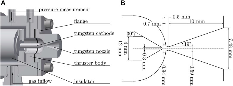
FIGURE 1. (A) Sectional view of the present nozzle geometry. (B) Schematic sectional view of the nozzle geometry.

2.3 Numerical mesh and case setup

2.3.1 Numerical meshes

For the numerical study, three meshes are used: two for the CSL DSMC simulations and one additional for the Navier–Stokes simulation. The numerical meshes for the CSL DSMC simulations are generated based on the geometrical data presented in Figure 1B. An outlet domain of 15 mm by 7.5 mm is added to the nozzle to consider the downstream effects of boundary conditions on the nozzle flow plume and backflow effects. The application of an inlet domain was considered but rejected because no changes in flow properties could be observed after a certain distance upstream of the nozzle’s throat. The nozzle flow is considered axial symmetric. Hence, wedge meshes with an opening angle of 2.5° are used. The lower resolution mesh for the CSL DSMC simulations is shown in Figure 2, whereas only every 4^th mesh line (not refined parts) is shown for accurate presentation. For the CSL DSMC simulations, mesh refinement is carefully applied to the stagnation part and the second half of the diffuser to achieve optimized parallel performance and higher numerical resolution on the nozzle’s exit plane (see red marked areas in Figure 2). According to Bird, the cell size Δ x for a baseline DSMC simulation should be chosen smaller than the local mean free path λ (Bird, 1994). As a selection limiter technique is used in the study, this strict limitation is softened and replaced by more classical restrictions of continuum-based theory as proposed by Titov and Levin (2007). For mass flow rates of 0.178 mg/s $\le \dot{m}\le$ 3.568 mg/s, the coarser mesh shown in Figure 2 is used. For a mass flow rate of $\dot{m}=3.568$ mg/s, the cell size is set to three times the appropriate size for a baseline DSMC simulation. With declining mass flow rates, the factor Δ x/λ decreases, reaching a value of 0.2 for $\dot{m}=0.178$ mg/s. With refinement, the overall number of cells is 81,000, whereas the radial resolution at the throat and in the diffuser is 20 cells for the not refined parts and 40 cells for the refined parts. For mass flow rates larger than $\dot{m}=3.568$ mg/s, a finer mesh is used. Including refinement, the overall number of cells is 21,5000, whereas the radial resolution at the throat and in the diffuser is equivalent to the coarser mesh. For the highest studied experimental mass flow rate of $\dot{m}=71.360$ mg/s, the cell size of the pressurized part of the nozzle is set to approximately 49 times what would have been appropriate when performing a baseline DSMC simulation. With declining mass flow rates, with lower stagnation pressures, the ratio again decreases to Δ x/λ ≈ 5 for $\dot{m}=7.136$ mg/s. For the baseline DSMC simulations, separate numerical meshes are used for each mass flow rate. The meshes were generated in a manner that a factor of Δ x/λ ≤ 0.8 was reached for each of the simulations.

FIGURE 2

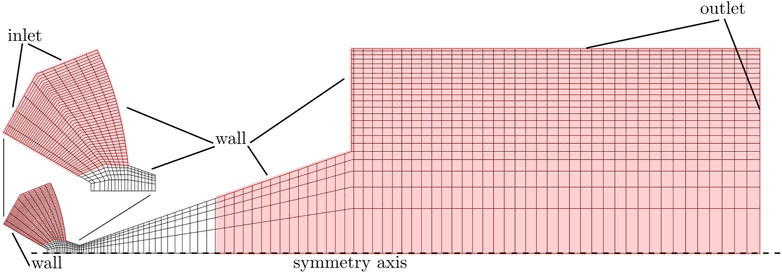
FIGURE 2. Numerical mesh of the thruster nozzle with an applied downstream domain. Only every 4^th meshline is displayed. Inlet, outlet, and wall surfaces are marked. Red background coloring indicates areas where the mesh is refined.

To improve numerical stability for the Navier–Stokes simulations, the outlet domain of the third mesh is scaled up to 60 mm by 40 mm. Mesh convergence was previously tested with six different grid resolutions (Table 1). The coarsest had 15 by 10 cells in the nozzle’s throat area, whereas the finest had 360 by 40 cells in the same area. In all cases, the cell size for the rest of the mesh was scaled according to the throat area. The referenced cell height is scaled by the throat radius r_* = 0.295 mm (Figure 1B). Tested mass flow rates were $\dot{m}=3.568$ mg/s and $\dot{m}=71.360$ mg/s. Final simulations are performed on the mesh with the highest resolution, with an overall number of 67,000 cells, because a neglectable change in flow properties was observed here. The computed stagnation pressure data are normalized with the measurement data in Table 4. Based on the documented changes in stagnation pressure, how the pressure converges with the example of the deviations from measurement results using increasingly finer grids can be seen. The converging deviations to the measured data are mass flow dependent. Deviations at the highest mass flows of approximately 0.5% are within the error range of the sensors.

TABLE 1

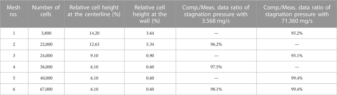
TABLE 1. Grid resolution and stagnation pressure convergence study. Tested meshes and data of the convergence study for Navier–Stokes simulations. The dimensionless cell height at the throat is given for the centerline and for the cell closest to the nozzle wall, whereat the cell height is scaled by the throat radius r_*. Data for numerical stagnation pressures are scaled by the experimental values for the two investigated mass flow rates to give a dimensionless pressure relation.

2.3.2 Case setup and boundary conditions

Two sets of boundary conditions are used for the numerical simulations. As given in Eq. 1, the number of per-time-step initialized particles at the inlet surface for the DSMC simulations are calculated from experimental mass flow rates $\dot{m}$ and the molecular properties of the gas. The particles are initialized with no macroscopic flow velocity according to an inlet temperature based on the experimental stagnation temperature T₀. Particle collisions with the solid walls of the domain are performed by applying diffusive Maxwellian scattering to the collided particles. The wall temperature T_w is set according to T₀. The outflow is modeled on the basis of Bird’s (1994) equilibrium formulation with the given experimental background pressures and ambient temperatures. The flow velocity is additionally set to u_out = 2,000 m/s out of the domain to prevent the non-physical accumulation of particles at the stream-wise outlet surface. The side planes of the mesh reflect simulation particles in a specular manner. The variable hard-sphere model is used to perform binary particle collisions. The number of simulation particles representing real molecules is adjusted to at least five particles per cell throughout the nozzle (Bird, 2007). No radial weighting of simulation particles is used, and global time steps Δ t are set in accordance with Table 2 for the CSL DSMC simulations. The ratios of Δ t/t_c, in which t_c = 1/ν is the mean collision time of a molecule, vary between 0.22 and 6.96 over the whole range of studied mass flow rates. In the baseline DSMC simulations, the time step is adjusted to Δ t/t_c ≤ 0.8 for each case. Molecular properties for argon, reference viscosity index, and diameter, as well as mass, are taken from Bird (1994). For the Navier–Stokes simulations, the mass flow into the numerical domain is modeled by an equivalent inflow velocity. The mass flow rate boundary conditions are adapted transiently for this purpose. By starting with approximately 2.5 times the targeted value, the mass flow rate decreases linearly until the desired mass flow rate is reached and thereafter kept constant to that value. Inflow temperature is set as experimentally obtained. Pressure at the outlet surfaces is modeled with a total pressure condition. Velocity at the solid walls is set to be constant zero, which leads to a no-slip boundary condition at the surface, whereas an adiabatic wall temperature condition is applied to consider cooling effects by the flow. An example of the boundary conditions used for the two solvers is shown in Table 3.

TABLE 2

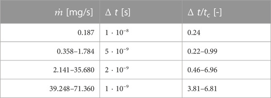
TABLE 2. Used time steps and ratios Δ t/t_c in the CSL DSMC simulations.

TABLE 3

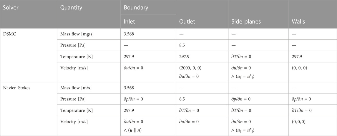
TABLE 3. Overview of the two sets of boundary conditions for the DSMC and the compressible Navier–Stokes simulations.

For the Navier–Stokes simulations, the specific heat capacity of argon is specified to c_p = 520 J/kg K (VDI, 2013) and the molar mass to 39.95 kg/kmol (VDI, 2013). The temperature-dependent dynamic viscosity μ is calculated using Sutherland’s law (Sutherland, 1893) as follows:

$\mu =\frac{A_s{T}^{3/2}}{T+T_s},(5)$

where T is the temperature, T_s is the Sutherland temperature, and A_s is the Sutherland coefficient. For the results presented here, the Sutherland coefficient and temperature are calculated using experimental data from Clarke and Smith (1968). The obtained values are A_s = 1.9487 ⋅ 10⁻⁶ Pa s/$\sqrt{\text{K}}$ and T_s = 144.8247 K.

3 Results

3.1 Physical description of the nozzle flow

The numerical study presented in this work is based on an experimental series of argon mass flow rates performed on the presented thruster. Mass flow rates range from $\dot{m}=0.178$ mg/s to $\dot{m}=71.360$ mg/s, covering two orders of magnitude. The pressure inside the thruster is hereby recorded by differential pressure sensors. Simultaneously, the background pressure p_vac is recorded. The pressure drop Δ p is added to the background pressure to receive the absolute stagnation pressure p_s of the thruster. Thrust and specific impulse are measured by a thrust balance. A complete overview of the experimental series is given in Table 4.

TABLE 4

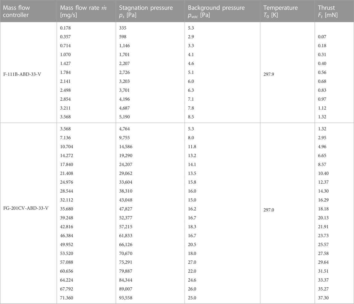
TABLE 4. Overview of the experimental series with argon.

For each of the experimentally investigated mass flow rates, numerical results are obtained using both methods. Altogether, 86 simulations were performed, giving a good data basis for the numerical investigation. Both solvers reached a steady state after a simulated time of approximately 3.5 m and were continued until a simulated time of approximately 6 m.

For the investigated range of mass flow rates, flow conditions from a continuum with Knudsen numbers below Kn = 0.01 to free flow conditions with Knudsen numbers over Kn = 10 are observed. For the highest mass flow rates, close to atmospheric conditions are reached inside the thruster, whereas plume flow conditions are in the free molecular range. Figure 3A shows the average Knudsen numbers obtained from baseline DSMC and CSL DSMC simulations at the nozzle’s throat and the exit plane over the range of investigated mass flow rates.

FIGURE 3

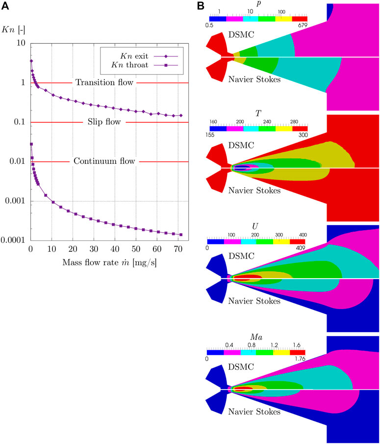
FIGURE 3. (A) Average throat and exit plane Knudsen numbers as a function of mass flow rates. (B) Pressure, temperature, velocity, and Mach number fields for a mass flow rate of $\dot{m}=0.357$ mg/s argon. Top half of each flow field: baseline DSMC solution, bottom half Navier–Stokes solution.

A clear dependency of the Knudsen number on the mass flow rate is seen. In the throat region of the thruster, Knudsen numbers stay in the continuum flow range for almost all investigated mass flow rates—the only exceptions are seen for the two smallest mass flow rates. In contrast, average exit plane values of the Knudsen number do not reach continuum flow or slip flow conditions, indicating that continuum-based assumptions may not be valid anymore.

As a result of the strong rarefaction of the flow, large deviations in numerical flow field distributions between the two solvers for pressure, velocity, temperature, and Mach number are present in Figure 3B for a mass flow rate of $\dot{m}=0.357$ mg/s argon. The scales provided for velocity, temperature, and Mach Number are adjusted to the range of baseline DSMC results to achieve comparability, whereas those for the pressure distribution are scaled to the Navier–Stokes results and displayed logarithmically.

The top picture presents the pressure drop along the nozzle. As a result of the large ratio of inlet area A_in to throat cross-section A_*, the pressure keeps almost constant until the beginning of the converging nozzle throat, and most of the pressure drop occurs at the end of the throat and the beginning of the diffuser. The generated stagnation pressures close to the inlet differ by approximately 11% from each other, whereas the DSMC simulation indicates a faster pressure drop in the diffuser compared to the Navier–Stokes solver.

Results for the velocity distribution show a gentle acceleration of the fluid close to the nozzle throat with further acceleration throughout the diffuser in agreement with de Laval Nozzle theory. For the selected mass flow rate, the highest velocities are already reached in the first 20% of the diffuser, which indicates a non-ideal ratio of mass flow rate to diffuser length. Radial velocity distribution and the velocities at the diffuser walls differ significantly, with slip flow present in the DSMC solution caused by strong rarefaction effects of the expanding flow.

By accelerating the fluid, internal thermal energy is converted to kinetic energy, leading to a drop in temperatures in the diffuser. The lowest temperatures are reached where the highest velocities are present. Toward the end of the diffuser, the temperature distribution of the Navier–Stokes solution recovers faster toward ambient temperature.

The distribution of the Mach number separates the nozzle in a sub- and supersonic part. In accordance with the de Laval nozzle theory, Ma = 1 is reached at the end of the nozzle’s throat in both solutions. Then, the Mach number increases as the flow expands into the diffuser, reaching maximum values where velocity approaches maximum values and temperature is minimal.

3.2 Overprediction of stagnation pressure

To analyze the applicability of the proposed CSL DSMC, numerical and experimental stagnation pressures are compared for the full range of studied mass flow rates. Discussion of results is split to mass flow ranges of 0.178 mg/s $\le \dot{m}\le$ 3.568 mg/s and 3.568 mg/s $\le \dot{m}\le$ 71.360 mg/s. Relative deviations between experimental and CSL DSMC results for the stagnation pressure are, for example, calculated by

${\delta }_{p_s}=\frac{p_{s,Exp}-p_{s,Num}}{p_{s,Exp}}\cdot 100\%.(6)$

3.2.1 Lower mass flow rates

The left part of Figure 4 shows the results for stagnation pressures of the CSL DSMC and the Navier–Stokes solver in comparison to experimental values for mass flow rates of 0.178 mg/s $\le \dot{m}\le$ 3.568 mg/s. On the right side of the figure, corresponding deviations are displayed. The Navier–Stokes solver strongly overpredicts experimental stagnation pressures for mass flow rates of 0.178 mg/s $\le \dot{m}\le$ 1.070 mg/s. The largest deviation of about 21% is present for the lowest mass flow rate of $\dot{m}=0.178$ mg/s and then rapidly decreases toward a mass flow rate of about $\dot{m}=1.070$ mg/s, after which only minor deviations scatter between 1.2% and 1.8%.

FIGURE 4

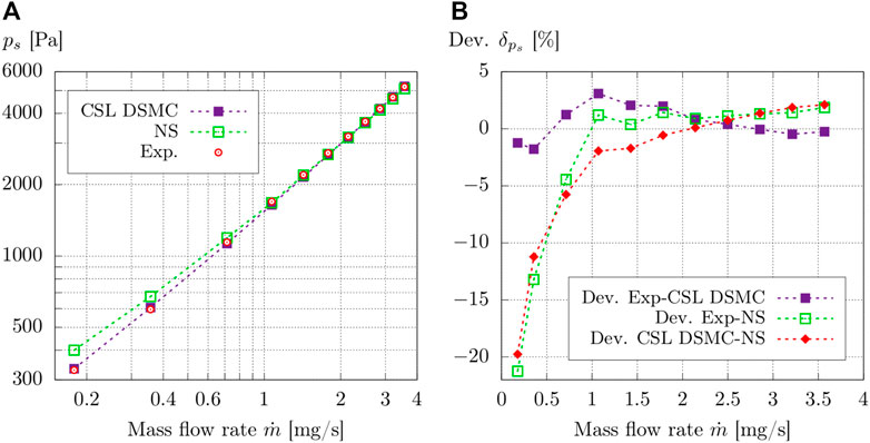
FIGURE 4. (A) Numerical and experimental stagnation pressures p_s for mass flow rates of 0.178 mg/s $\le \dot{m}\le$ 3.568 mg/s. (B) Deviations between numerical and experimental results over mass flow rates.

As the CSL DSMC solver can predict viscous losses more precisely for the strongly rarefied flow of the lower mass flow rates, deviations to experimental results are much smaller. For the two lowest measured mass flow rates, a slight overprediction of approximately 1.5% of the stagnation pressure is present for the CSL DSMC results. For mass flow rates of 0.714 mg/s $\le \dot{m}\le$ 2.498 mg/s, the CSL DSMC solver slightly underpredicts the stagnation pressure, with the largest deviation of 3.1% to experimental values present for a mass flow rate of $\dot{m}=1.070$ mg/s. For the three highest studied mass flow rates in Figure 4, the CSL DSMC solver again slightly overpredicts the experimental stagnation pressure, but deviations are as small as 0.5%.

A reasonable relation is observed between the numerical results of the CSL DSMC and Navier–Stokes simulations, showing that with decreasing mass flow rates, the rarefaction effects of the flow exhibit a level the Navier–Stokes solver can handle, leading to apparent higher stagnation pressures in comparison to the CSL DSMC results. For mass flow rates over $\dot{m}=2.141$ mg/s, the relation is switching to, in comparison, slightly higher stagnation pressures obtained by the CSL DSMC solver.

3.2.2 Higher mass flow rates

In the left part of Figure 5, stagnation pressures of the CSL DSMC and the Navier–Stokes solutions are shown for mass flow rates of 3.568 mg/s $\le \dot{m}\le$ 71.360 mg/s. A growing overprediction of the stagnation pressure by the CSL DSMC solver is seen with rising mass flow rates, whereas the Navier–Stokes solver almost perfectly reproduces the stagnation pressure over the full range of experimental values. A closer look at deviations is given on the right side of Figure 5. Although an apparent deviation of 7% is present between experimental and Navier–Stokes results for the lowest mass flow rate of $\dot{m}=3.568$ mg/s, the remainder of examined mass flow rates are excellently reproduced by the continuum approach. Deviations between the Navier–Stokes results and the experimental data may reach 2.1% for a mass flow rate of $\dot{m}=21.408$ mg/s, but in general, the slight underprediction of the stagnation pressure by the Navier–Stokes solver is almost negligible.

FIGURE 5

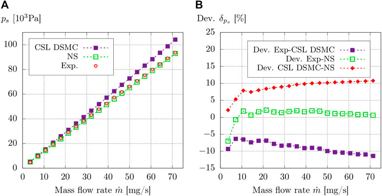
FIGURE 5. (A) Numerical and experimental stagnation pressures p_s for mass flow rates of 3.568 mg/s $\le \dot{m}\le$ 71.360 mg/s. (B) Deviations between numerical and experimental results over mass flow rates.

In contrast, the CSL DSMC results for the stagnation pressure do not reproduce the experimental values or the Navier–Stokes results. Although a decreasing overprediction from 9.3% to 6.4% of the experimental value is seen for the two lowest mass flow rates of $\dot{m}=3.568$ mg/s and $\dot{m}=7.136$ mg/s, the deviation rises again for mass flow rates of 7.136 mg/s $\le \dot{m}\le$ 71.360 mg/s. The highest deviation of 11.4% is reached, with the highest mass flow rate investigated.

CSL DSMC and Navier–Stokes results are compared in Figure 5 to better understand the influence of the selection limiter scheme on the stagnation pressure and exclude possible errors from the experiment. By starting with a deviation of 2.1% at the handover mass flow rate of $\dot{m}=3.568$ mg/s, the deviation more than doubles (5.3%) with a twice as high mass flow rate of $\dot{m}=7.136$ mg/s. However, the increase in deviation is not linear with the mass flow rate, and for a 10 times larger mass flow rate of $\dot{m}=71.360$ mg/s, the deviation only roughly doubles to 10.8%.

3.2.3 Slowed down velocity relaxation

The deviations of the CSL DSMC results for the stagnation pressure from both experimental and numerical Navier–Stokes results are best explained regarding the centerline profiles of scaled density ρ/ρ₀, temperature T/T₀, and velocity U/U_max in Figure 6, where density ρ and temperature T are scaled by the stagnation values ρ₀ and T₀ of the CSL DSMC simulation, whereas the velocity profiles are scaled by the maximum velocity U_max reached by the particular CSL DSMC simulation. The axial position is scaled by the throat radius r_* = 0.295 mm (Figure 1B), where zero indicates the throat position and a value of x/r_* = 30 the nozzle’s exit plane.

FIGURE 6

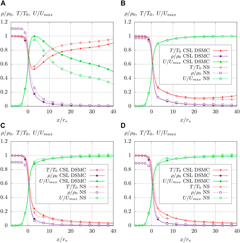
FIGURE 6. Centerline profiles of scaled density ρ/ρ₀, temperature T/T₀, and velocity U/U_max obtained by the CSL DSMC solver (continuous lines) and the Navier–Stokes solver (dashed lines) for four different mass flow rates. (A) $\dot{m}=0.357$ mg/s, (B) $\dot{m}=3.568$ mg/s, (C) $\dot{m}=35.680$ mg/s, (D) $\dot{m}=71.360$ mg/s.

Due to the rarefaction of the flow for $\dot{m}=0.357$ mg/s, a strong non-equilibrium is present in the viscous boundary layer of flow, which leads to non-zero wall velocities. This effect is only mapped by the CSL DSMC solver because no slip boundary conditions are applied to the Navier–Stokes simulations and wall velocities tend to zero close to the wall. As a result, the viscous losses in the boundary region, calculated by the CSL DSMC solver, are lower than the one predicted by the continuum theory-based Navier–Stokes solver. The higher kinetic energy in the diffuser with higher maximum centerline velocities in the CSL DSMC solution leads to less thermal energy, which results in lower centerline temperatures in the core flow compared to the Navier–Stokes solution. Due to the higher viscous losses predicted by the Navier–Stokes solver, the transition from thermal to kinetic energy and vice versa is slowed down, leading to an increase in the stagnation density and consequently to too high stagnation pressures p_s for the smaller mass flow rates in Figure 4.

With rising mass flow rates, Knudsen numbers in Figure 3A decrease to a level where no major effects on flow properties due to flow rarefaction can be seen on the centerline profiles for $\dot{m}=3.568$ mg/s in Figure 6. In contrast to a mass flow rate of $\dot{m}=0.357$ mg/s, the stagnation density ρ/ρ₀ reached by the Navier–Stokes solver is a bit lower than the one obtained by the CSL DSMC solver, with a deviation of approximately 2% regarding Figure 4 within experimental uncertainty.

Regarding higher mass flow rates of $\dot{m}=35.680$ mg/s and $\dot{m}=71.360$ mg/s in Figure 6, a major change in the centerline profiles is seen as 0 ≤ x/r_* ≤ 10. Here, the CSL DSMC results deviate strongly from the Navier–Stokes solution. Although the Navier–Stokes solver predicts local maxima and minima for the centerline values, the CSL DSMC solution does not capture this effect. The explanation for that behavior is found in the applied selection limiter scheme. As collisions are limited to two collisions per test particle per time step, velocity relaxation is slowed down if the local velocity distribution in the cell is far from the equilibrium condition. As a result, more time steps are necessary to achieve a local and a macroscopic change of velocity, and the acceleration of the fluid at the beginning of the diffuser is slowed down. This behavior was also found by Titov and Levin (2007) and Titov et al. (2008), and it vanishes if a baseline DSMC simulation with proper time step and cell size is used, which is also why the phenomena are not seen for the lower displayed mass flow rates of $\dot{m}=0.357$ mg/s and $\dot{m}=3.568$ mg/s in Figure 6. In contrast, the effect increases when the time steps and cell sizes are increased compared to a baseline DSMC simulation. As velocity, temperature, and density are coupled, the effect is also seen on the centerline temperature and density. As a result of the slowed-down velocity relaxation, too high stagnation densities and consequently stagnation pressures p_s are obtained by the CSL DSMC solver with deviations to experimental and Navier–Stokes results up to 11% for a mass flow rate of $\dot{m}=71.360$ mg/s.

3.2.4 Impact of the wall accommodation coefficient on predicted stagnation pressure

The impact of different wall accommodation coefficients σ_v on the stagnation pressure p_s is investigated, as a variation of the coefficient may enhance the flow rate by raising the flow velocity close to the nozzle wall. Wall accommodation coefficients σ_v of 1.0, 0.9, 0.8, and 0.5 are investigated. A value of σ_v = 1.0 represents a fully diffusive reflection of particles from the wall, with an average tangential velocity of zero. For an assumed value of σ_v = 0.0, particles would be reflected in a specular manner, resulting in an inviscid flow with zero friction at the wall. As it can be assumed that the value of σ_v = 0.0 does not represent the physical flow, the lowest investigated value is σ_v = 0.5, where approximately half of the particles are scattered diffusively and specularly.

Table 5 presents obtained stagnation pressures from CSL DSMC simulations and relative deviations to experimental values for different accommodation coefficients for four mass flow rates. As can be seen, a steady decline of numerically obtained pressure for all mass flow rates is present when the coefficient is lowered. The lowest pressures are reached for σ_v = 0.5. In comparison to experimentally obtained stagnation pressures, two major effects can be seen. For the lower mass flow rates up to $\dot{m}=3.568$ mg/s, a value of σ_v between 0.9 and 0.8 may improve the pressure results, closing the gap between experimental and numerical results for a CSL DSMC simulation. With a value of σ_v = 0.5, stagnation pressures with too low values are obtained. For the higher displayed mass flow rates of $\dot{m}=35.680$ mg/s and $\dot{m}=71.360$ mg/s, only minor relative changes to the pressure are present. Even applying a value of σ_v = 0.5 still leads to a significant overprediction of stagnation pressure. Since the overall impact of different values of σ_v does not highly improve the pressure results, and for easier comparison, a value of σ_v = 1.0 is applied in this study.

TABLE 5

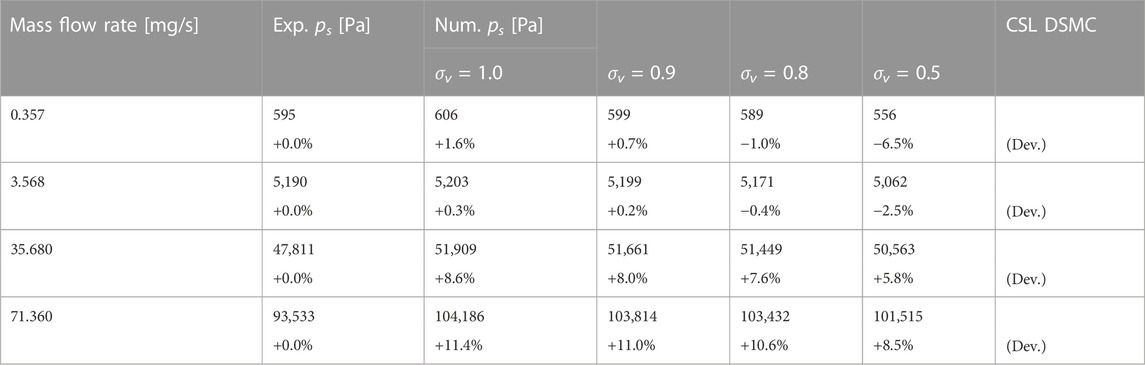
TABLE 5. Stagnation pressures of CSL DSMC simulations for different wall accommodation coefficients and mass flow rates.

4 Discussion

4.1 Comparison to baseline DSMC simulations

The overprediction of the stagnation pressure for the higher mass flow rates present in the CSL DSMC simulations should vanish if a DSMC simulation in accordance with the baseline criteria is applied. Hence, results for the CSL DSMC and Navier–Stokes simulations are compared to baseline DSMC simulations. Four mass flow rates of 0.357, 1.780, 3.568, and 7.136 mg/s are studied.

Table 6 presents results for the experimentally obtained stagnation pressure and for the three solvers. For the lowest mass flow rate of 0.357 mg/s, by applying the selection limiter scheme, no change in results for the pressure is present between baseline and CSL DSMC simulations. Deviations may only be within numerical uncertainty because baseline criteria for the time step and cell size are met in both simulations. The Navier–Stokes simulation clearly overpredicts the stagnation pressure.

TABLE 6

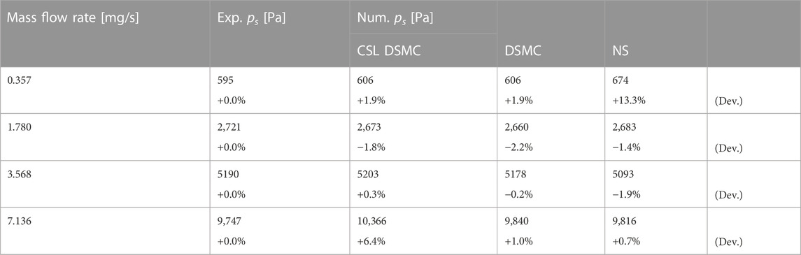
TABLE 6. Comparison of stagnation pressures of CSL DSMC, baseline DSMC, and NS simulations for mass flow rates between 0.357 and 7.136 mg/s.

For mass flow rates of 1.780 and 3.568 mg/s, only a little change in the stagnation pressure can be observed once again, comparing both CSL and baseline DSMC simulations. For 1.780 mg/s, both the DSMC and the Navier–Stokes simulations slightly underpredict the experimental value but within experimental error. However, a slight decrease of 0.4% can be seen regarding stagnation pressures for the CSL and baseline DSMC simulations. Regarding the results for a mass flow rate of 3.568 mg/s, a slight decrease of 0.5% in the stagnation pressure is obtained. Here, the effects of the selection limiter, enlarged time steps, and cell sizes may begin to show.

For the highest mass flow rate of 7.136 mg/s, shown in Table 6, the CSL DSMC simulation clearly overpredicts the experimental stagnation pressure of approximately 6.4% due to the applied selection limiter scheme. In contrast to that, the baseline DSMC simulation can predict the stagnation well, with a minor overprediction of approximately 1.0%, reaching almost the value of the Navier–Stokes simulation. Deviations between baseline DSMC and Navier–Stokes results may be within numerical uncertainty.

Table 6 shows that the effect of stagnation pressure overprediction vanishes if a baseline DSMC simulation is applied. The effects of the proposed selection limiter scheme and comparison to baseline DSMC simulations are also analyzed regarding centerline profiles of scaled flow properties, presented in Figure 7. For the lowest mass flow rate of 0.357 mg/s, no visible deviation between CSL and baseline DSMC is present over the whole nozzle. Even for mass flow rates of 1.780 and 3.568 mg/s, CSL and baseline DSMC basically predict the same profiles for scaled density ρ/ρ₀, temperature T/T₀, and velocity U/U_max. The small deviations in stagnation pressures shown in Table 6 may be present for the two mass flow rates.

FIGURE 7

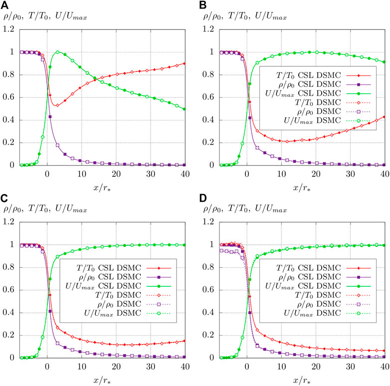
FIGURE 7. Centerline profiles of scaled density ρ/ρ₀, temperature T/T₀, and velocity U/U_max obtained by CSL DSMC simulations (continuous lines) and the baseline DSMC simulations (dashed lines) for four different mass flow rates. (A) $\dot{m}=0.357$ mg/s, (B) $\dot{m}=1.780$ mg/s, (C) $\dot{m}=3.568$ mg/s, (D) $\dot{m}=7.136$ mg/s.

In contrast, deviations between CSL and baseline DSMC are present for a mass flow rate of 7.136 mg/s in Figure 7. As a result of the full velocity relaxation, the baseline DSMC simulation reaches slightly lower centerline densities ρ/ρ₀ and higher velocities U/U_max directly after the nozzle throat at 0 ≤ x/r_* ≤ 10. This, in return, leads to lower stagnation densities ρ/ρ₀ and lower stagnation pressure obtained for the baseline DSMC simulation in Table 6 for 7.136 mg/s.

4.2 Thrust and specific impulse prediction

The second analysis of interest for the applicability is conducted on the dependency of predicted thrust and specific impulse using the CSL scheme. As differences between pressure values at the nozzle’s exit plane and measured background pressures of the far field are small for all examined mass flow rates, the effects of additional pressure drop on the generated thrust are neglected, and the numerical thrust for both used solvers is calculated by

$F_{t,num}={\int }_A\rho \vec{u}\left(\vec{u}\cdot \vec{n}\right)\mathrm{d}A,(7)$

where ρ is the density, $\vec{u}$ the velocity, and $\vec{n}$ the normal vector of the exit plane. Regarding Eq. 7, the specific impulse I_sp can be computed by the mass flow rate $\dot{m}$ and the thrust force F_t with

$I_{\mathbf{sp}}=\frac{F_t}{\dot{m}g}.(8)$

Numerically and experimentally obtained thrust forces for the investigated range of mass flow rates are shown on the left side of Figure 8. The lowest thrust forces are obtained for a mass flow rate of $\dot{m}=0.357$ mg/s, and a maximum value of approximately 37 mN is reached with a mass flow rate of $\dot{m}=71.360$ mg/s.

FIGURE 8

FIGURE 8. (A) Exit plane thrust F_t. (B) Deviations between obtained thrust forces.

With 0.357 mg/s $\le \dot{m}\le$ 2.854 mg/s on the left side of Figure 8, the Navier–Stokes solver strongly underpredicts the thrust with deviations up to 40% because the impact of flow rarefaction is evident. Regarding a mass flow rate of $\dot{m}=0.357$ mg/s shown in Figure 6, due to the higher predicted viscous losses along the diffuser by the Navier–Stokes approach, the centerline velocity profile becomes lower. Although the Navier–Stokes solution generates higher densities, the lower velocities lead to a reasonable decrease in calculated thrust, as shown in Figure 8.

With a rising mass flow rate, the deviation between numerical results decreases rapidly, reaching a value of under 2.5% for $\dot{m}=2.854$ mg/s of argon and final deviations to under 1% for mass flow rates up to $\dot{m}=71.360$ mg/s. In comparison to experimental thrust forces, both solvers reproduce the experimental thrust very well for mass flow rates of 10.704 mg/s $\le \dot{m}\le$ 71.360 mg/s. Regarding the right side of Figure 8, for the highest examined mass flow rates, the CSL DSMC results are a bit closer and relative deviations to experimental values are smaller. For mass flow rates smaller than $\dot{m}=1.427$ mg/s, the deviation between the Navier–Stokes solution and experimental values is rapidly rising. However, some relative deviations between numerical and experimental results are present for both solvers of 1.427 mg/s $\le \dot{m}\le$ 10.704 mg/s, which may be explained by measurement error of the mass flow controller.

In summary, the CSL DSMC solver reproduces the experimental thrust better over the whole range of mass flow rates, which is remarkable as the results in Section 3.2 show an overprediction of the stagnation pressure caused by the applied selection limiter scheme for the higher mass flow rates. However, the pressure overprediction does not seem to have a huge effect on predicted thrust values, meaning that the study of exit plane and plume data is valid. An explanation for that behavior is given in Figure 9, showing the evolution of numerical thrust throughout the normalized diffuser length D_n.

FIGURE 9

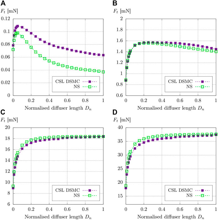
FIGURE 9. Evolution of thrust over the normalized length of the diffuser D_n for mass flow rates of (A) $\dot{m}=0.357$ mg/s, (B) $\dot{m}=3.568$ mg/s, (C) $\dot{m}=35.680$ mg/s, (D) $\dot{m}=71.360$ mg/s.

Two major effects can be seen in Figure 9. For the smallest displayed mass flow rate of $\dot{m}=0.357$ mg/s, it is evident that rarefaction effects of the flow are present in the whole diffuser, which leads to an underprediction of thrust by the Navier–Stokes solver. In addition, maximum thrust forces for both solvers are already reached within the first 5% of the diffuser. For the ten times larger mass flow rate, both solvers reproduce the thrust well, whereas a light deviation in predicted thrust is seen in the second half of the diffuser, indicating the beginning of the breakdown of the continuum approach, confirmed by the exit plane Knudsen numbers in Figure 3A.

In contrast, deviations based on the application of the selection limiter are present for $\dot{m}=35.680$ mg/s and $\dot{m}=71.360$ mg/s in Figure 9. Caused by the slowed-down velocity relaxation in the CSL DSMC simulations, the flow along the diffuser is decelerated, and maximum velocities, as well as corresponding thrust forces, are reached later in the diffuser. However, toward the end of the diffuser, Navier–Stokes thrust values are mapped by the CSL DSMC simulations with deviations less than 1%.

Figure 10A shows the results for the specific impulse I_sp as a function of mass flow rate. As previously pointed out for the thrust forces in Figure 8, the apparent deviation between the two numerical results is present for mass flow rates below $\dot{m}=2.854$ mg/s. For the higher mass flow rates, deviations again decrease and are considered negligible and within the statistical scatter of numerical results. For the higher mass flow rates, viscous losses at the nozzle walls prevent the flow from further acceleration, approaching the adiabatic limit for a cold-gas expansion. As a result, the present growth of the specific impulse is seen in Figure 10A for that range of mass flows, and the growth of the thrust in Figure 8 is only attributed to the rising mass flow.

FIGURE 10

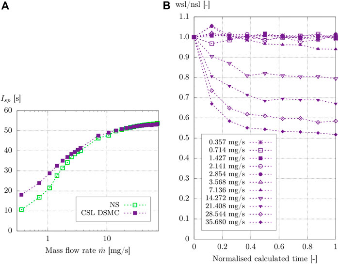
FIGURE 10. (A) Calculated exit plane specific impulses I_sp for the CSL DSMC and the Navier–Stokes solver. (B) Relative computational speed-up.

4.3 Computational performance characterization of the scheme

The computational speed-up as a function of normalized calculated time for different mass flow rates is displayed in Figure 10B to characterize the performance. The dimensionless speed-up wsl/nsl is calculated as a fraction of two simulations, one with activated CSL (wsl) and one without (nsl). However, mesh size and time step are unaltered.

For displayed mass flow rates of 0.357 mg/s $\le \dot{m}\le$ 3.568 mg/s, no computational speed up is present because limitations for time step meet the requirements of a baseline DSMC simulation, and subsequently, the calculated number of collision partners is low in comparison to the cut-off number of two collisions per particle per cell. For mass flow rates of 7.136 mg/s $\le \dot{m}\le$ 35.680 mg/s, a growing influence and speed-up of the cut-off collision number are seen on the computational time. The highest speed-up of wsl/nsl = 0.51, and consequently, the largest computational saving are present for the highest mass flow rate and largest calculated time.

5 Conclusion

An argon cold gas flow through a millimeter-scaled thruster nozzle geometry with high-density ratios was experimentally and numerically investigated using a compressible Navier–Stokes solver and a DSMC solver with a modified collisional routine, here denoted as CSL. To evaluate the applicability of the CSL DSMC for nozzle flow investigations, mass flow rates of 0.178 mg/s $\le \dot{m}\le$ 71.360 mg/s are studied, generating flow conditions from continuum flow to free flow.

The comparison of the numerical results with experimentally obtained stagnation pressures shows a clear overprediction by the Navier–Stokes solver for cases with rarefied gas flow and mass flow rates of 0.178 mg/s $\le \dot{m}\le$ 1.070 mg/s. For mass flow rates above $\dot{m}=1.070$ mg/s, the Navier–Stokes solver reproduces the stagnation pressure almost perfectly with only minor deviations, which is in accordance with the continuum-based theory.

In contrast, the DSMC method with applied CSL can reproduce the stagnation pressure well for the lower mass flow rates due to the kinetic nature of the method. By applying the CSL, the DSMC method overpredicts the stagnation pressure with rising mass flow rates up to a deviation of 11.4% from the experimental value for the largest mass flow rate studied. The impact of the wall accommodation coefficient is studied. A value of 0.9 to 0.8 for the coefficient could slightly improve results for the stagnation pressure for the lower mass flow rates. By applying a baseline DSMC simulation, the effects of the selection limiter scheme vanish, and the stagnation pressure is predicted correctly.

However, the results of the thrust and specific impulse prediction show that the applied CSL scheme does not alter the results, and the CSL DSMC can reproduce the experimental thrust and specific impulse for the higher mass flow rates. Results are in excellent agreement with the Navier–Stokes and experimental results. In addition, studied cases with lower mass flow rates, which are shown to be clearly in the rarefied flow regime, are naturally and correctly predicted by the CSL DSMC method.

Despite an overprediction of stagnation pressures, the CSL DSMC method is a suitable tool for predicting thrust and a specific impulse of cold gas micro-nozzle flows through the whole range of flow regimes.

By applying the CSL scheme, computational speed-up factors up to 0.51, dependent on the mass flow rate, could be achieved in the CSL DSMC simulations.

Data availability statement

The raw data supporting the conclusion of this article will be made available by the authors, without undue reservation.

Author contributions

TF and RG contributed to the conception and design of the study. TF performed the numerical computation. TF wrote the first draft of the manuscript. TF and RG wrote sections of the manuscript. All authors contributed to the manuscript revision and read and approved the submitted version.

Funding

The “North-German Supercomputing Alliance” (HLRN) provided computational time for the numerical study in this work (Funding ID: hbi00027).

Acknowledgments

The authors would like to thank Fionn Zeidler for his support in performing the numerical parameter studies and processing the simulation results.

Conflict of interest

The authors declare that the research was conducted in the absence of any commercial or financial relationships that could be construed as a potential conflict of interest.

Publisher’s note

All claims expressed in this article are solely those of the authors and do not necessarily represent those of their affiliated organizations or those of the publisher, the editors, and the reviewers. Any product that may be evaluated in this article, or claim that may be made by its manufacturer, is not guaranteed or endorsed by the publisher.

Footnotes

¹BRONKHORST HIGH-TECH B.V., Nijverheidsstraat 1A, NL-7261 AK Ruurlo (NL).

²First Sensor AG, Peter-Behrens-Straße 15, 12459 Berlin, Germany.

³Vision Engineering Ltd., Anton-Pendele-Str. 3, 82275 Emmering, Deutschland.

References

Alexeenko, A., Levin, D., Gimelshein, S., Collins, R., and Reed, B. (2002). Numerical modeling of axisymmetric and three-dimensional flows in microelectromechanical systems nozzles. AIAA J. 40, 897–904. doi:10.2514/3.15139

CrossRef Full Text | Google Scholar

Bartel, T., Sterk, T., Payne, J., and Preppernau, B. (1994). “Dsmc simulation of nozzle expansion flow fields,” in 6th Joint Thermophysics and Heat Transfer Conference, Colorado Springs, CO. doi:10.2514/6.1994-2047

CrossRef Full Text | Google Scholar

Bird, G. (1994). Molecular gas dynamics and the direct simulation of gas flows, vol. 42. Oxford, UK: Oxford Engineering Science Series, Clarendon Press.

Google Scholar

Bird, G. (2007). “Sophisticated dsmc,” in Notes prepared for a short course at the DSMC07 meeting, Santa Fe, USA.

Google Scholar

Boyd, I., Chen, G., and Candler, G. (1995). Predicting failure of the continuum fluid equations in transitional hypersonic flows. Phys. Fluids 7, 210–219. doi:10.1063/1.868720

CrossRef Full Text | Google Scholar

Boyd, I., Ketsdever, A., and Muntz, E. (2003). Predicting breakdown of the continuum equations under rarefied flow conditions. AIP Conf. Proc. 663, 899–906. doi:10.1063/1.1581636

CrossRef Full Text | Google Scholar

Burt, J., and Boyd, I. (2009). A hybrid particle approach for continuum and rarefied flow simulation. J. Comput. Phys. 228, 460–475. doi:10.1016/j.jcp.2008.09.022

CrossRef Full Text | Google Scholar

Burt, J., and Boyd, I. (2008). A low diffusion particle method for simulating compressible inviscid flows. J. Comput. Phys. 227, 4653–4670. doi:10.1016/j.jcp.2008.01.020

CrossRef Full Text | Google Scholar

Busse, C., Tsivilskiy, I., Hildebrand, J., and Bergmann, J. P. (2021). Numerical modeling of an inductively coupled plasma torch using openfoam. Comput. Fluids 216, 104807. doi:10.1016/j.compfluid.2020.104807

CrossRef Full Text | Google Scholar

Clarke, A., and Smith, E. (1968). Low-temperature viscosities of argon, krypton, and xenon. J. Chem. Phys. 48, 3988–3991. doi:10.1063/1.1669725

CrossRef Full Text | Google Scholar

Frieler, T., and Groll, R. (2018). A torsional sub-milli-Newton thrust balance based on a spring leaf strain gauge sensor. Rev. Sci. Instrum. 89, 075101. doi:10.1063/1.4996419

PubMed Abstract | CrossRef Full Text | Google Scholar

Gomez, J., and Groll, R. (2016). Pressure drop and thrust predictions for transonic micronozzle flows. Phys. Fluids 28, 022008. doi:10.1063/1.4942238

CrossRef Full Text | Google Scholar

Gorji, M., and Jenny, P. (2015). Fokker–planck–dsmc algorithm for simulations of rarefied gas flows. J. Comput. Phys. 287, 110–129. doi:10.1016/j.jcp.2015.01.041

CrossRef Full Text | Google Scholar

Greenshields, C. J., Weller, H. G., Gasparini, L., and Reese, J. (2010). Implementation of semi-discrete, non-staggered central schemes in a colocated, polyhedral, finite volume framework, for high-speed viscous flows. Int. J. Numer. Methods Fluids 63, 1–21.

Google Scholar

Groll, R., Fastabend, F., and Rath, H. (2012). “Modelling transsonic flows through ring-shape thruster geometries with dsmc,” in ASME 2012 10th International Conference on Nanochannels, Microchannels, and Minichannels (New York City, USA: American Society of Mechanical Engineers (ASME)), 195–204.

CrossRef Full Text | Google Scholar

Groll, R., and Gomez, J. (2016). Identifying microproduction inaccuracies with knudsen number depending correction functions. AIP Conf. Proc. 1786, 080012. doi:10.1063/1.4967605

CrossRef Full Text | Google Scholar

Ivanov, S., Markelov, N., Kashkovsky, V., and Giordano, D. (1997). Numerical analysis of thruster plume interaction problems. Eur. Spacecr. Propuls. Conf. 398, 603.

Google Scholar

Ketsdever, A., Lilly, T., Gimelshein, S., and Alexeenko, A. (2005). Experimental and numerical study of nozzle plume impingement on spacecraft surfaces. Tech. rep. DTIC Document.

Google Scholar

Kolobov, V., Arslanbekov, R., Aristov, V., Frolova, A., and Zabelok, S. A. (2007). Unified solver for rarefied and continuum flows with adaptive mesh and algorithm refinement. J. Comput. Phys. 223, 589–608. doi:10.1016/j.jcp.2006.09.021

CrossRef Full Text | Google Scholar

Kühn, C., and Groll, R. (2021). picfoam: An openfoam based electrostatic particle-in-cell solver. Comput. Phys. Commun. 262, 107853. doi:10.1016/j.cpc.2021.107853

CrossRef Full Text | Google Scholar

Kurganov, A., Noelle, S., and Petrova, G. (2001). Semidiscrete central-upwind schemes for hyperbolic conservation laws and Hamilton–Jacobi equations. SIAM J. Sci. Comput. 23, 707–740. doi:10.1137/s1064827500373413

CrossRef Full Text | Google Scholar

Kurganov, A., and Tadmor, E. (2000). New high-resolution central schemes for nonlinear conservation laws and convection–diffusion equations. J. Comput. Phys. 160, 241–282. doi:10.1006/jcph.2000.6459

CrossRef Full Text | Google Scholar

Macrossan, M. (2001). A particle simulation method for the bgk equation. AIP Conf. Proc. 585, 426–433. doi:10.1063/1.1407592

CrossRef Full Text | Google Scholar

Muraviev, A., Bashinov, A., Efimenko, E., Volokitin, V., Meyerov, I., and Gonoskov, A. (2021). Strategies for particle resampling in pic simulations. Comput. Phys. Commun. 262, 107826. doi:10.1016/j.cpc.2021.107826

CrossRef Full Text | Google Scholar

Roohi, E., Darbandi, M., and Mirjalili, V. (2009). Direct simulation Monte Carlo solution of subsonic flow through micro/nanoscale channels. J. heat Transf. 131, 092402. doi:10.1115/1.3139105

CrossRef Full Text | Google Scholar

Scanlon, T., Roohi, E., White, C., Darbandi, M., and Reese, J. (2010). An open source, parallel dsmc code for rarefied gas flows in arbitrary geometries. Comput. Fluids 39, 2078–2089. doi:10.1016/j.compfluid.2010.07.014

CrossRef Full Text | Google Scholar

Shang, Z., and Chen, S. (2013). 3d dsmc simulation of rarefied gas flows around a space crew capsule using openfoam. Open J. Appl. Sci. 3, 35–38. doi:10.4236/ojapps.2013.31005

CrossRef Full Text | Google Scholar

Sharma, A., and Long, L. N. (2004). Numerical simulation of the blast impact problem using the direct simulation Monte Carlo (dsmc) method. J. Comput. Phys. 200, 211–237. doi:10.1016/j.jcp.2004.03.015

CrossRef Full Text | Google Scholar

Sutherland, W. (1893). Lii. the viscosity of gases and molecular force. Lond. Edinb. Dublin Philosophical Mag. J. Sci. 36, 507–531. doi:10.1080/14786449308620508

CrossRef Full Text | Google Scholar

Titov, E., Kumar, R., Levin, D., Gimelshein, N., Gimelshein, S., and Abe, T. (2008). Analysis of different approaches to modeling of nozzle flows in the near continuum regime. AIP Conf. Proc. 1084, 978. doi:10.1063/1.3076619

CrossRef Full Text | Google Scholar

Titov, E., and Levin, D. (2007). Extension of the dsmc method to high pressure flows. Int. J. Comput. Fluid Dyn. 21, 351–368. doi:10.1080/10618560701736221

CrossRef Full Text | Google Scholar

Titov, E., Zeifman, M., and Levin, D. (2005a). “Application of the kinetic and continuum techniques to the multi-scale flows in mems devices,” in 43rd AIAA Aerospace Sciences Meeting and Exhibit, 1399. doi:10.2514/6.2005-1399

CrossRef Full Text | Google Scholar

Titov, E., Zeifman, M., and Levin, D. (2005b). “Examination of new dsmc methods for efficient modeling of mems device flows,” in 4th AIAA Theoretical Fluid Mechanics Meeting, Toronto, Ontario, 6–9. AIAA Paper. vol. 5058. doi:10.2514/6.2005-5058

CrossRef Full Text | Google Scholar

VDI (2013). VDI-Wärmeatlas. 11 edn. Berlin: Springer Vieweg.

Google Scholar

Wang, W., Sun, Q., Boyd, I., Ketsdever, A., and Muntz, E. (2003). Assessment of a hybrid method for hypersonic flows. AIP Conf. Proc. 663, 923–930. doi:10.1063/1.1581639

CrossRef Full Text | Google Scholar

Yu, S., Wu, H., Xu, J., Wang, Y., Gao, J., Wang, Z., et al. (2023). A generalized external circuit model for electrostatic particle-in-cell simulations. Comput. Phys. Commun. 282, 108468. doi:10.1016/j.cpc.2022.108468

CrossRef Full Text | Google Scholar

Zelesnik, D., Micci, M., and Long, L. (1994). Direct simulation Monte Carlo model of low Reynolds number nozzle flows. J. Propuls. Power 10, 546–553. doi:10.2514/3.23807

CrossRef Full Text | Google Scholar

Zhang, R., Yao, W., and Li, J. (2008). A selection limiter of dsmc for near continuum flows. Commun. Nonlinear Sci. Numer. Simul. 13, 2203–2212. doi:10.1016/j.cnsns.2007.06.004

CrossRef Full Text | Google Scholar