Dynamics and control analysis during rendezvous in non-Keplerian Earth—Moon orbits

The paper describes the development of a framework capable of addressing some fundamental issues in the analysis of proximity operations between two spacecraft that are operating within a three-body model defined by two primaries and the spacecraft themselves. The main objective is to enable the capability of analysing dynamic and control issues during an automated rendezvous between a vehicle and a passive space station orbiting around the Earth - Moon L2 Lagrangian point on a near rectilinear halo orbit. The paper presents first a restricted three body model dynamics and a nominal approach trajectory, followed by an analysis of the influence of assumed actuators and sensors. Critical aspects such as selected failures are investigated, in order to ensure passive safety of the mission using impulsive maneuvers. An example of closed loop guidance in the near range is also presented and the overall performance are validated with an Ephemeris model available in the literature.

1 Introduction

The paper describes the development of a framework capable of addressing fundamental issues in the dynamic analysis of proximity operations between two spacecraft that are operating within a three-body model defined by the gravitational influence of two primaries. The main motivation for the work is the planned return to the Moon with the construction of station orbiting a near rectilinear halo orbit around the L2 libration point and the subsequent rendezvous operations between vehicles leaving the satellite to reach the station and/or coming from Earth. The scenario is under study by several space agencies, with the cooperation of private industries, in the US, Canada, Europe, and China among others. Examples of early studies are the Heracles project by ESA Landgraf (2019), Renk et al. (2018) (now replaced by ESA EL3 program) and the more consolidated Artemis project sequence NASA (2015).

The proposed location of a permanent station (currently named Lunar Gateway) requires the extension of preliminary dynamic analysis from Keplerian motion to a three-body restricted model setting. In this context, relative motion between an active chaser spacecraft and a passive Gateway is casted into elliptical and circular restricted three-body problems, in their non-linear and linearized versions. The working scenario for validation considers a maneuver starting from about 100 km distance between the two vehicles with an open loop impulsive guidance strategy during the far away approach and closed loop control in the final phase when relative distance is less than 1 km. The overall trajectory is divided into several waypoints (or hold points) necessary for state evaluation and sensor suite modification. The actuation in each interval assumes a two-impulse procedure. Extensive simulation is performed leading to a high confidence level in the selection of the rendezvous location near the aposelene of the Gateway orbit and use of a linearized circular restricted three-body model accurate enough for guidance computation.

In order to increase the fidelity of the simulation, an investigation was carried out by adding sensors and actuators models to the relative dynamics. Performance of the propagation equations over more orbit periods were analyzed and compared to available Ephemeris data present in the literature.

One of the critical issues in the development of the far distance guidance was the optimization of the number and location of waypoints, to evaluate energy expenditure and to guarantee passive safety of the maneuver. This analysis was a result of a non-linear optimization based on the definition of safety areas around the Gateway. Extensive Montecarlo simulation demonstrated the capability of selecting waypoints different from the initial location, which would provide safety and guarantee the possibility of a new rendezvous approach procedure after one orbit of the space station, when a number of critical actuator failures could occur. The paper also presents a proposed closed loop guidance strategy during the final phase of the rendezvous. The selected algorithms use an optimal technique based on state dependent Riccati equations for the relative translation and classical PID controller for the attitude dynamics. The selection of closed loop control was performed for validation purposes and not necessarily to achieve the best solution. Finally, the proposed work was evaluated by creating a comprehensive simulation tool (ROSSONERO), which allows the mission planner to examine the performance capabilities of the design within the assumed constraints, to investigate alternate solutions in the presence of failures and a comparison with results achievable using Ephemeris. The paper is organized as follows: Section 2 describes the working scenario, Section 3 analyzes different models and evaluates their validity in terms for guidance purposes. Section 4 describes a general view of potential errors introduced by assuming selected sensors and actuators with specified dynamics. Open loop guidance design is studied in Section 5 with respect to failures, which could prevent rendezvous, whereas Section 6 describes a potential approach to closed loop guidance in the vicinity of the target. The software developed for this work is briefly described in Section 8, followed by conclusions.

2 Working scenario

The paper is based on a specific rendezvous scenario, which can be generalized to many actual situations occurring during the Gateway life span in the next decade. Permanent return to the Moon requires a deep space station that would operate as intermediary between Earth and lunar surface operations. Early studies can be found in Whitley and martinez R. (2016), Whitley and Martinez (2018), Howell (2001), where candidate halo orbits were considered. The selection of a near rectilinear halo orbit (NRHO) has several advantages such as a continuous link with Earth, and the capability of communicating with the dark side of our satellite, among others, while needing limited propulsion expenditure for station keeping. In this work, a Southern L2 9:2 resonance halo orbit is considered as reference and depicted in Figure 1. The orbital properties assumed in the paper are: period of 6.56 days, periselene at 1,500 km and aposelene at 70,000 km.

FIGURE 1

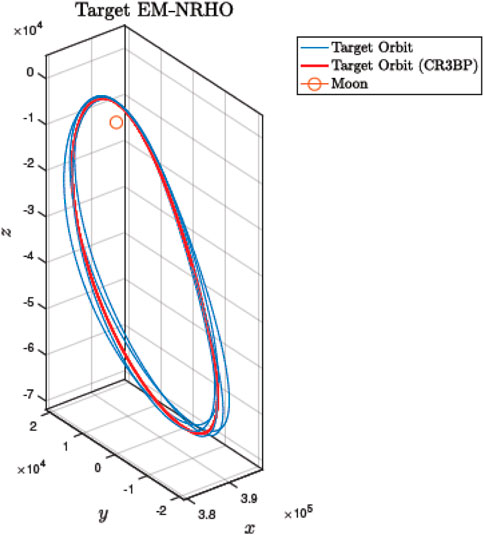
FIGURE 1. Reference Target Orbit and its Propagation in the Synodic Reference Frame.

The relative motion dynamics in this work are those between the passive orbiting Gateway (target) and an active lunar Ascender Element (LAE or chaser), which departed the lunar surface, and must perform an automated rendezvous starting from an assumed distance of about 100 km, until berthing can be executed. The rendezvous trajectory is divided into a sequence of hold points, necessary for status evaluation, sensor management, and definition of potentially necessary impulsive maneuvers, if mission control warrants it. The actual LAE configuration is not critical for this study, and it is taken from available data in: Innocenti and Bucchioni (2019). It consists of a cylindrical body of about 2.6 m of diameter, with a main engine, 16 attitude thrusters, and a berthing hook located at some specified point. Figure 2 shows the qualitative trajectory section of the Heracles mission that is considered in this paper.

FIGURE 2

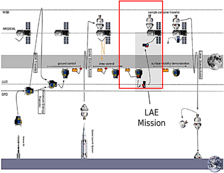
FIGURE 2. Rendezvous maneuver example (courtesy of ESA).

3 Relative motion dynamics

This section describes the relative motion equations and the assumptions made. The primary focus is the necessity of considering the gravitational influence of both Earth and Moon on the LAE, and the potential advantages of the circular restricted three body problem hypothesis with the applicability of manifold theory Koon et al. (2011), Lizy-Destrez et al. (2019), Ueda et al. (2017), Topputo (2015).

Spacecraft relative dynamics is a critical aspect in rendezvous and docking, formation flight, debris mitigation, in-orbit assembly and servicing. Relative motion in the two-body problem has been studied extensively since the 1960’s, see for instance, Clohessy and Wiltshire (1960), Tschauner and Hempel (1965). Important contributions can also be found in Fehse (2003), Gurfil and Seidelmann (2016), and Ankersen (2011), among others. The study of relative motion in a three body scenario is not as widespread and new interest has stemmed in the past decade from specific missions such as the Phobos sample return project and of course the return to the Moon. Some examples in the literature are Lizy-Destrez et al. (2019), Bucci et al. (2017) and Colagrossi and Lavagna (2018).

Although in many instances the CR3BP model may be sufficiently accurate, there are cases where elliptic motion is of interest, therefore the equations of relative motion are presented in both versions. In addition, the Local Vertical Local Horizon (LVLH) frame is also used, because of its convenience from the guidance, navigation and control point of view. The results presented herein are taken by previous work by the authors and details can be found primarily in Innocenti and Franzini (2018), and Innocenti et al. (2022).

3.1 Reference frames

This section reviews the reference frames used in the paper, with the three body hypothesis used due to the presence of two primaries. The equations or relative motion (see Wie (2008)) are based on the following standard reference frames Innocenti and Franzini (2018):

• Inertial Frame [C, Î, Ĵ, K ̂ ]. The inertial frame is centered at the primaries common center of mass C, with the K̂ unit vector normal to the plane where the primaries revolve. The other unit vectors span the primaries rotating plane.

• Synodic Frame [C, î_m, ĵ_m, k̂_m]. The synodic frame is used to describe a spacecraft motion in a system with two main primary bodies. The origin of the frame is set at the Moon for convenience.

• Local Vertical Local Horizon (LVLH) Frame [C, î_L, ĵ_L, k̂_L]. The LVLH is a target centered frame, useful in the study of guidance and control issues. It simplifies the analysis of relative motion with respect to the chaser. We will refer to the tangential, normal and radial directions as V-bar, H-bar and R-bar, even though these unit vector names refer formally to Keplerian circular orbits.

The reference frames are depicted in Figure 3.

FIGURE 3

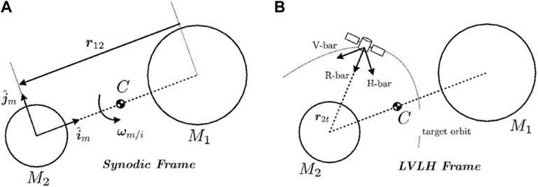
FIGURE 3. Non inertial reference frames Innocenti and Franzini (2018) (A) Synodic Frame. (B) LVLH Frame.

3.2 Relevant equations of motion

In the restricted three body problem, we assume that the spacecraft masses are negligible with respect to the mass of each primary. From Franzini and Innocenti (2019), Franzini and Innocenti (2017), and Bucchioni and Innocenti (2021b), the equations of relative motion in the LVLH frame and in nondimensional units are given in Eq. 1:

$\begin{array}{cc}\hfill {\left.\ddot{\mathit{\rho }}\right|}_{\mathcal{L}}=& -\mu \frac{\mathit{r}+\mathit{\rho }}{\Vert \mathit{r}+\mathit{\rho }{\Vert }^3}-\left(1-\mu \right)\left(\frac{\mathit{r}+\mathit{\rho }+{\mathit{r}}_{\mathit{e}\mathit{m}}}{\Vert \mathit{r}+\mathit{\rho }+{\mathit{r}}_{\mathit{e}\mathit{m}}{\Vert }^3}\right)\hfill \\ \hfill & +\mu \frac{\mathit{r}+\mathit{\rho }}{\Vert \mathit{r}{\Vert }^3}+\left(1-\mu \right)\left(\frac{\mathit{r}+{\mathit{r}}_{\mathit{e}\mathit{m}}}{\Vert \mathit{r}+{\mathit{r}}_{\mathit{e}\mathit{m}}{\Vert }^3}\right)\hfill \\ \hfill & -2{\mathit{\omega }}_{\mathit{l}/\mathit{i}}\times {\left.\dot{\mathit{\rho }}\right|}_{\mathcal{L}}-{\left.{\dot{\mathit{\omega }}}_{\mathit{l}/\mathit{i}}\right|}_{\mathcal{L}}\times \mathit{\rho }-{\mathit{\omega }}_{\mathit{l}/\mathit{i}}\times \left({\mathit{\omega }}_{\mathit{l}/\mathit{i}}\times \mathit{\rho }\right)\hfill \end{array}(1)$

where μ is the Earth-Moon mass parameter, ${\left.\dot{\mathit{\rho }}\right|}_{\mathcal{L}}$ and ${\left.\ddot{\mathit{\rho }}\right|}_{\mathcal{L}}$ are the relative velocity and acceleration as seen in the LVLH frame, ω_l/i and ${\left.{\dot{\mathit{\omega }}}_{\mathit{l}/\mathit{i}}\right|}_{\mathcal{L}}$ are the angular velocity and angular acceleration of the LVLH frame with respect to an inertial reference frame $\mathcal{I}$. The chaser position with respect to the Moon is given by r + ρ, and the Earth—Moon distance is r_em. The relationship between the different angular velocities is given by Eq. 2, where the subscripts l, m, and i indicate LVLH, synodic and inertial frames respectively.

${\mathit{\omega }}_{l/i}={\mathit{\omega }}_{l/m}+{\mathit{\omega }}_{m/i},{\left[{\dot{\mathit{\omega }}}_{l/i}\right]}_{\mathcal{L}}={\left[{\dot{\mathit{\omega }}}_{l/m}\right]}_{\mathcal{L}}-{\mathit{\omega }}_{l/m}\times {\mathit{\omega }}_{m/i}(2)$

For simplicity, orbital perturbations and solar pressure are not considered in this work.

Equation 1 can be simplified for guidance purposes if we consider the elliptic and circular approximations of the primaries with respect to their common center of mass. The elliptic non-linear equations of motion (ENERM) are shown below, and are considered representative of the exact dynamics in this work:

$\begin{array}{cc}\hfill {\left[\ddot{\mathit{\rho }}\right]}_{\mathcal{L}}& =-2{\mathbf{\Omega }}_{l/i}{\left[\dot{\mathit{\rho }}\right]}_{\mathcal{L}}-\left({\left[{\dot{\mathbf{\Omega }}}_{l/i}\right]}_{\mathcal{L}}+{\mathbf{\Omega }}_{l/i}^2\right)\mathit{\rho }+\mu \left(\frac{\mathit{r}}{r^3}-\frac{\mathit{r}+\mathit{\rho }}{\Vert \mathit{r}+\mathit{\rho }{\Vert }^3}\right)\hfill \\ \hfill & +\left(1-\mu \right)\left(\frac{\mathit{r}+{\mathit{r}}_{em}}{{‖\mathit{r}+{\mathit{r}}_{em}‖}^3}-\frac{\mathit{r}+\mathit{\rho }+{\mathit{r}}_{em}}{{‖\mathit{r}+\mathit{\rho }+{\mathit{r}}_{em}‖}^3}\right)\hfill \end{array}(3)$

Further simplification can be performed by linearizing the gravitational acceleration yielding the elliptic linear equations of motion (ELERM):

$\begin{array}{c}\hfill {\left[\ddot{\rho }\right]}_{\mathcal{L}}=-2{\mathbf{\Omega }}_{l/i}{\left[\dot{\mathit{\rho }}\right]}_{\mathcal{L}}-\left({\left[{\dot{\mathbf{\Omega }}}_{l/i}\right]}_{\mathcal{L}}+{\mathbf{\Omega }}_{l/i}^2+\frac{\mu }{r^3}\left(\mathit{I}-3\frac{\mathit{r}{\mathit{r}}^T}{r^2}\right)\right.\\ \hfill +\frac{1-\mu }{{‖\mathit{r}+{\mathit{r}}_{em}‖}^3}\left(\mathit{I}-3\frac{\left(\mathit{r}+{\mathit{r}}_{em}\right){\left(\mathit{r}+{\mathit{r}}_{em}\right)}^T}{{‖\mathit{r}+{\mathit{r}}_{em}‖}^2}\right)\mathit{\rho }\end{array}(4)$

In the above equations the terms Ω_l/i and ${\left[{\dot{\mathbf{\Omega }}}_{l/i}\right]}_{\mathcal{L}}$ are skew-symmetric matrices associated with angular velocity and acceleration ω_l/i and ${\left[{\dot{\mathit{\omega }}}_{l/i}\right]}_{\mathcal{L}}$, respectively. Using the circular restricted three body problem hypothesis, the above equations can be additionally simplified (see Franzini and Innocenti (2019) for details) by taking advantage of the representation of angular velocity and angular acceleration ω_l/i and ${\left[{\dot{\mathit{\omega }}}_{l/i}\right]}_{\mathcal{L}}$ in this particular case. This yields a set of non-linear and linear equations, denoted CNERM and CLERM respectively.

CLERM equations can also be written in a state space compact form affine in the control $\dot{\mathit{x}}(t)=\mathit{A}(t)\mathit{x}(t)+\mathit{B}\mathit{u}(t)$, which is a linear time-varying system, with:

$\begin{array}{cc}\hfill \mathit{x}\left(t\right)=& \left[\begin{array}{c}\hfill \mathit{\rho }\hfill \\ \hfill {\left.\dot{\mathit{\rho }}\right|}_{\mathcal{L}}\hfill \end{array}\right]\hfill \\ \hfill \mathit{A}\left(t\right)=& \left[\begin{array}{cc}\hfill {\mathit{O}}_{\mathit{3}\mathit{x}\mathit{3}}\hfill & \hfill {\mathit{I}}_{\mathit{3}\mathit{x}\mathit{3}}\hfill \\ \hfill {\mathit{A}}_{\mathbf{21}}\hfill & \hfill -2{\mathbf{\Omega }}_{\mathit{l}/\mathit{i}}\hfill \end{array}\right]\hfill \\ \hfill {\mathit{A}}_{\mathbf{21}}=& {\left.{\dot{\mathbf{\Omega }}}_{\mathit{l}/\mathit{i}}\right|}_{\mathcal{L}}+{\mathbf{\Omega }}_{\mathit{l}/\mathit{i}}^2-\frac{\mu }{\Vert {\mathit{r}}_{\mathit{m}\mathit{t}}{\Vert }^3}\left({\mathit{I}}_{\mathit{3}\mathit{x}\mathit{3}}-3\frac{{\mathit{r}}_{\mathit{m}\mathit{t}}{\mathit{r}}_{\mathit{m}\mathit{t}}^T}{\Vert {\mathit{r}}_{\mathit{m}\mathit{t}}{\Vert }^2}\right)\hfill \\ \hfill & -\frac{1-\mu }{\Vert {\mathit{r}}_{\mathit{m}\mathit{t}}+{\mathit{r}}_{\mathit{e}\mathit{m}}{\Vert }^3}\left({\mathit{I}}_{\mathit{3}\mathit{x}\mathit{3}}-3\frac{\left({\mathit{r}}_{\mathit{m}\mathit{t}}+{\mathit{r}}_{\mathit{e}\mathit{m}}\right){\left({\mathit{r}}_{\mathit{m}\mathit{t}}+{\mathit{r}}_{\mathit{e}\mathit{m}}\right)}^T}{\Vert {\mathit{r}}_{\mathit{m}\mathit{t}}+{\mathit{r}}_{\mathit{e}\mathit{m}}{\Vert }^2}\right.\hfill \\ \hfill \mathit{B}=& \left[\begin{array}{c}\hfill {\mathit{O}}_{\mathit{3}\mathit{x}\mathit{3}}\hfill \\ \hfill {\mathit{I}}_{\mathit{3}\mathit{x}\mathit{3}}\hfill \end{array}\right]\hfill \end{array}(5)$

The rationale behind the derivation is the analysis of their propagation and the identification of their validity according to the location of the Gateway along its orbit.

Using the reference scenario of ESA’s the Human Lunar Precursor Program (HLEPP) from Bucci et al. (2017), Renk et al. (2017), extensive Montecarlo simulations were carried out Franzini and Innocenti (2019), Innocenti and Franzini (2018) in order to compare propagated relative position and velocity errors, assuming the aposelene area as rendezvous location, which is where the Gateway has the lowest speed. The equation sets were compared using the following maximum distance and speed errors and an additional aggregate performance index.

The maximum distance and speed errors are defined as:

$e_p={\max }_{t\in \left[t_0,t_f\right]}\Vert \mathit{\rho }\left(t\right)-\widehat{\mathit{\rho }}\left(t\right)\Vert ,e_v={\max }_{t\in \left[t_0,t_f\right]}\Vert \dot{\mathit{\rho }}\left(t\right)-\dot{\widehat{\mathit{\rho }}}\left(t\right)\Vert (6)$

In the above equations the hat indicates the relative position and velocities calculated by the tested equation set, whereas the quantities without hat are the true values (that is the propagation of ENERM set).

The combined index of performance is:

$\nu ={\max }_{t\in \left[t_0,t_f\right]}\Vert \mathit{\xi }\left(t\right)-\widehat{\mathit{\xi }}\left(t\right)\Vert ,\mathit{\xi }=\left[\begin{array}{c}\hfill \mathit{\rho }\hfill \\ \hfill n\dot{\mathit{\rho }}\hfill \end{array}\right](7)$

The results were parametrized versus the mean n motion of the NRHO orbit, assuming an expression of the mean anomaly M given by:

$M\left(t\right)=2\pi \frac{t}{T}(8)$

This yields a range of mean anomaly of about M ∈ [80, 280] degrees, corresponding to the lower part of Figure 1.

A summary of the results is shown in Figures 4–6, where the colors from red to blue indicate poorer performance and large errors.

FIGURE 4

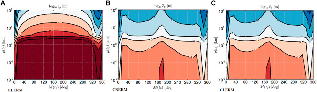
FIGURE 4. Average Position Error for different Models. (A) ELERM, (B) CNERM, (C) CLERM.

Figure 4 shows the increase in position error estimation introduced by the use of the circular restricted models CNERM and CLERM (non-linear and linear) with respect to the linear elliptic model (ELERM), however if we limit the region of motion near the aposelene the use of relative motion based on CR3BP can be considered appropriate for guidance and control purposes. Similar results are obtained by computing the aggregate performance index ν as depicted in Figure 5. Figure 6 shows the average errors in the rendezvous area. From the results, we can see that at the aposelene position errors are lower than 1 cm for distances lower than 100 m and 1 m for speed lower than 10 cm/s. This validates the use of CNERM and CLERM equation sets for the guidance design in the final phase. Results for the ENERM model are not presented, since it is assumed to be the “perfect” model, thus without errors.

FIGURE 5

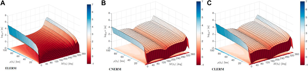
FIGURE 5. Aggregate performance index for ELERM, CNERM and CLERM models. (A) ELERM, (B) CNERM, (C) CLERM.

FIGURE 6

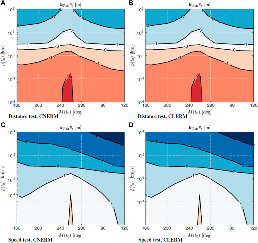
FIGURE 6. Average Position and Speed Errors in the Rendezvous Zone using the CR3BP Models. (A) Distance test, CNERM. (B) Distance test, CLERM. (C) Speed test, CNERM. (D) Speed test, CLERM.

3.3 Phasing

This subsection presents a simulated evaluation of the performance of the equations of relative motion as derived previously. The analysis is carried out with a preliminary computation of a phasing trajectory, although this part of the mission is not strictly considered within rendezvous constraints.

The LAE vehicle considered in this work will depart the lunar surface in the direction of the Gateway, and will reach the rendezvous conditions after a phasing maneuver. Phasing is a commonly used orbit transfer, which in many cases reduces the energy consumption with respect to a direct trajectory. Phasing trajectories can be computed using different methods, for instance minimum fuel consumption, specific time interval for the transfer. The computation complexity depends directly on the dynamic model used in the design. In cislunar setting, the design of this maneuver requires the non-negligible gravitational effects of Earth and Moon. Examples can be found in Bucchioni and Innocenti (2021b), Bucci et al. (2017), Shang et al. (2015), Blazquez et al. (2018b), Blazquez et al. (2018a), and Gomez et al. (2001). For the present analysis, the boundary conditions for the phasing trajectory were taken as follows:

• Initial orbit: circular LLO at 100 km altitude and 90° inclination (polar orbit).

• Insertion point: 50 km below the target (near the aposelene) and more than 86 km behind the target (so that the initial distance is greater than 100 km as the chaser begins the rendezvous towards the target).

The phasing described in the paper consists of the analysis of a direct transfer using a two-impulse maneuver with initial conditions determined solving a two-body Lambert’s problem, from a direct Hohmann transfer and a gradient-based optimization with multiple firings Bucchioni and Innocenti (2021a). Based on a CR3BP model, the resulting transfer trajectory was injected into a stable manifold generated by the target orbit, and selected in the direction of the eigenvector associated with the relevant eigenvalue of the appropriate Monodromy matrix. The comparison of the different approaches is summarised below. Afterwards, an analysis with an ER3BP model was carried out in order to evaluate the levels of approximation.

Figure 7 shows an example of phasing trajectory using Lambert’s problem. The stable manifold is propagated from an 80 km perturbation and it is met at the aposelene. The final position error is zero since we are on the desired manifold. The time of flight of the phasing trajectory is 78.5 h (half period of the target orbit) and the total expenditure is ΔV = 660 m/s. Note the out-of-plane phasing result, which warrants further analysis beyond the scope of the paper.

FIGURE 7

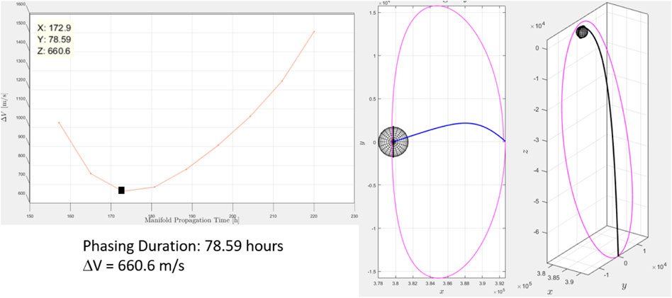
FIGURE 7. Direct Phasing with Lambert’s first Guess Bucchioni and Innocenti (2021a).

Figure 8 an example of resulting trajectory with a Hohmann transfer initial guess. Again the stable manifold is propagated from an 80 km perturbation with the aposelene intersection. As in the previous case, the final position error is zero. The time of flight is similar to the previous case (half period of the target orbit) and the total expenditure is ΔV = 671 m/s.

FIGURE 8

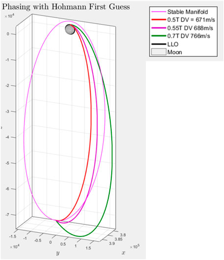
FIGURE 8. Direct Phasing with Hohmann first Guess Bucchioni and Innocenti (2021a).

For the of multiple impulse optimization, there is no differential correction, there are position errors at the final time, whose entities depend on the propagation equations and optimization stopping conditions. The optimization used is gradient-based, with a quadratic performance index that weighs the position error and the fuel expenditure, as shown in Eq. 9.

$\mathbf{J}=Q_1‖{\mathbf{e}‖}^2+Q_2{\left(\sum _i\Vert \mathrm{\Delta }{V}_i\Vert \right)}^2(9)$

where e is the error between final and desired states,

$\mathbf{e}={\mathbf{x}}_{\mathit{fin}}^{\mathit{Syn}}-{\mathbf{x}}_{\mathit{des}}^{\mathit{Syn}}(10)$

and ΔV_i are the fuel expenditures for each impulse. The scalar weights Q₁ and Q₂ are user selectable depending on the relative importance of the cost components.

Based on extensive simulation Innocenti et al. (2020), the best results were obtained for a 4-impulse sequence and different stable manifolds were evaluated in terms of their ΔV requirements. The best results for ΔV were 688 and 687 m per second for a manifold propagation of one orbital period (80 km and 100 km perturbations). The phasing trajectory with a time of flight of half orbital period is depicted in Figure 9.

FIGURE 9

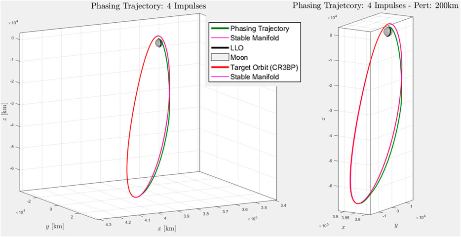
FIGURE 9. Direct phasing trajectory with a 4-impulse firing Innocenti et al. (2020).

A longer time of flight and manifold propagation may lead to a reduction in the final position error and ΔV. This can be seen in Figure 10, for instance, where a five period manifold propagation and time of flight of 29 days 5 h 2 min yield a position error within the requirements and a ΔV = 678.401 m/s.

FIGURE 10

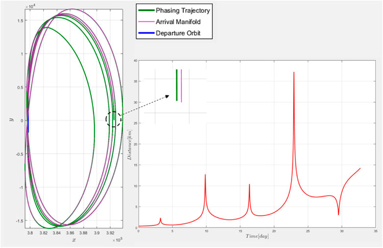
FIGURE 10. Direct Phasing Trajectory with a 5 period Orbit Propagation and TOF of 29d 5 h 2 m.

Finally, Figure 11 shows the modification of the phasing trajectory, when propagation is performed using the ER3BP model described in Eq. 1. Periodicity of the NRHO is now obviously lost, and for a time of flight of half period, the expenditure resulted in a ΔV = 703 m/s. The figure also shows the loss of accuracy at the periselene as the propagation time increases. The validity of CR3BP is limited to a time of flight much lower than the propagation time as expected.

FIGURE 11

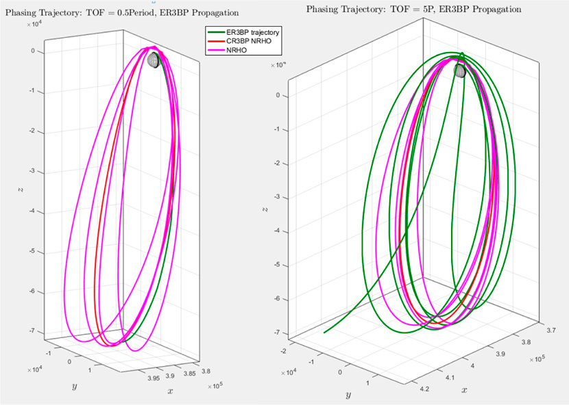
FIGURE 11. Phasing trajectory with ER3BP equations: 0.5P (left), 5P (right) propagation.

The analysis described above resulted in a ΔV expenditure consistent with recent NASA results as shown in May et al. (2020), in which the authors achieved bounds of the order of 680 <ΔV <880 m per second, depending on the time of flight of phasing.

4 Influence of sensor and actuator models

One of the aspects of interest in this work was the analysis of models of sensors and actuators in the propagation of the equations of relative dynamics described in Section 3. To this end, keeping in mind the scope of the paper, some of the assumed sensors and actuators used in the LAE dynamics are briefly reviewed and their behavior evaluated with respect to perfect modeling in a sample rendezvous trajectory, based on the mission scenario described in Section 2.

4.1 Sensor models

The set of sensors used by the guidance and control depends on the relative distance between the two vehicles, which is defined by the location of the hold points. This provides the active suite at any particular moment. A general behavioral model may have the form Ankersen (2011):

${\mathbf{x}}_m\left(t\right)={\mathbf{T}}_x\left(\mathbf{I}+\mathbf{k}\right)\mathbf{x}\left(t-\tau \right)+{\mathbf{b}}_x\left(t-\tau \right)+{\mathbf{n}}_x\left(t-\tau \right)(11)$

where: x is the model state vector, T is the misalignment, k the scale-factor, b_x the drift,n_x stochastic noise and delays given by τ. In general, d_x, n_x and τ are not constant in time and space. A critical role in the mission is played by the cameras that give distance and attitude information, in addition to standard measurements provided by inertial and star based units. A qualitative description of the sensor suites used depending on the distance between the vehicles is shown in Figure 12. Due to the objectives of the paper, we only give an overview of the relationship between cameras and relative distance as function of measurement errors.

FIGURE 12

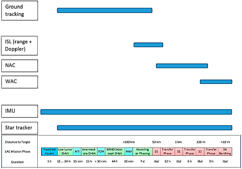
FIGURE 12. Qualitative Description of relevant Sensors Bucchioni and Innocenti (2021b).

The cameras reference variables used for distance and attitude are shown in Figure 13 and they are based on typical values provided by the sixth and seventh authors. In the figure, l is the target length, assumed equal to 5 m, α_c is the measured target center of mass azimuth angle, affected by an error of 100% of the target illuminated size, α₁ is the difference between the azimuth of the center of the illuminated zone and the azimuth of a side of the illuminated zone and ang_px the pixel angular size of the visible target area. The primary range measurement for large distances comes from the inter satellite link (ISL radio and/or radar), whereas wide angle and narrow angle cameras take over (WAC, NAC) at closer distances. Details on the numerical properties for ISL, WAC, and NAC can be found in Bucchioni and Innocenti (2021b), Ankersen (2011) and D. C. Woffinden (2007).

FIGURE 13

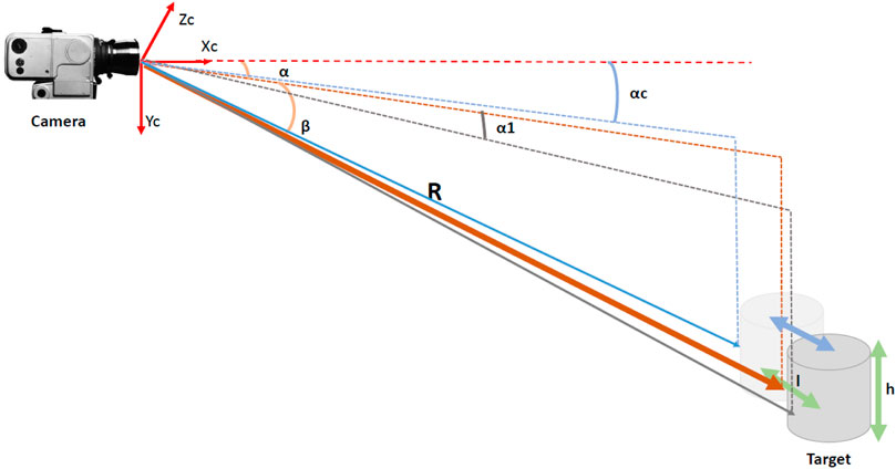
FIGURE 13. Reference quantities and camera frame Innocenti et al. (2020).

At large distances (more than 10 km), the range is measured by the ISL, with an assumed estimation error typically of the order of 3%R, which is lower than the error by the NAC, as shown in Figure 14 left. The error was computed using Eq. 12.

$RangeErro{r}_{\%}=0.5\frac{an{g}_{px}}{2{\alpha }_1}100(12)$

FIGURE 14

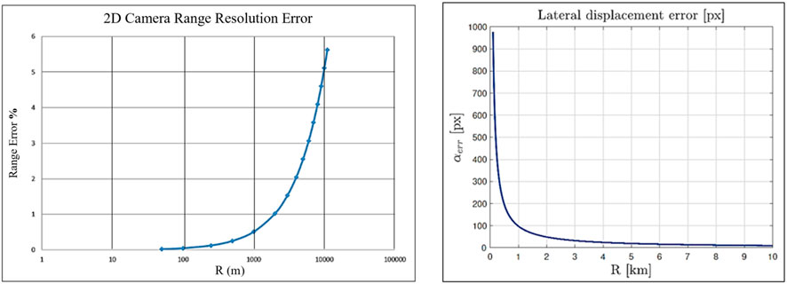
FIGURE 14. Range (left) and Lateral (right) Errors Estimates vs. Distance.

For medium distances (between 10 km and 1 km) the range is estimated using the NAC using Eq. 13.

$R_{\mathit{err}}=\frac{l}{2}\left(\frac{\cos {\alpha }_c}{\tan {\alpha }_1}+\sin {\alpha }_c\right)\pm 0.5\frac{an{g}_{px}}{2{\alpha }_1}(13)$

The narrow angle camera can also measure the lateral displacement (α and β), which includes a 100% error of the target angular visible size (about 1-2px) for large distance compensation. This error is computed using Eq. 14 and the its trend is depicted in Figure 14 right.

${\alpha }_{\mathit{err}}=\arctan \frac{l}{R}(14)$

The angle α_err specifies the limits between medium and short distances. Medium distance is assumed that for which $RangeErro{r}_{\%}$ is less than 3%R but the lateral displacement error is less than 100px, as a result, the medium distances are in the range 10km-1km.

The short distances are those defined between 1 km and 5 m. The sensor used is the wide angle camera WAC; the error on lateral displacement is about 0.2%R while the error on relative distance (downrange) R is 2%R. At short distances the relative attitude can also be estimated with a maximum error of the order 5°.

The estimation of the translational velocity is based on the differentiation principle and a subsequent Kalman filtering procedure, however, in this work, the entire navigation chain is modelled as in Eq. 15.

$\widetilde{\stackrel{̇}{{\rho }_{pp}}}=\dot{{\rho }_{pp}}+\Vert \widetilde{{\rho }_{pp}}-{\rho }_{pp}\Vert {\mathbf{n}}_{\dot{{\rho }_{pp}}}(15)$

with $\widetilde{\stackrel{̇}{{\rho }_{pp}}}$ the relative port-to-port velocity affected by the error, $\dot{{\rho }_{pp}}$ the velocity without errors, $\widetilde{{\rho }_{pp}}$ the relative position affected by error, ρ_pp the relative position and ${\mathbf{n}}_{{\dot{\rho }}_{pp}}$ is a white noise.

Similarly, the angular velocity error is given by Eq. 16

$\tilde{\omega }=\omega +\Vert \tilde{\theta }-\theta \Vert {\mathbf{n}}_{\omega }(16)$

The variables with tilde are the estimated ones, both ${\mathbf{n}}_{\dot{\rho }}$ and n_ω characteristics can be selected by the user.

A better understanding of the influence of the measurements is shown in Figure 15. This example describes a port-to-port trajectory to the Gateway in the V-bar direction. The accuracy of the models is clear.

FIGURE 15

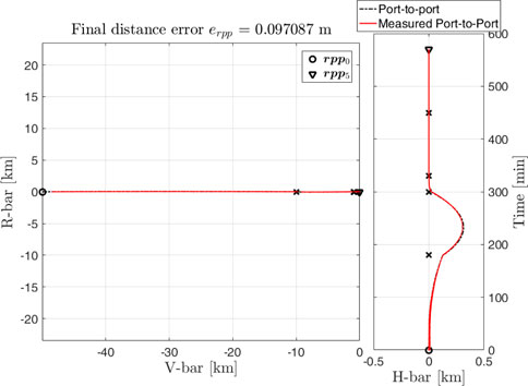
FIGURE 15. Port-to-Port Maneuver with the measured Range.

Obviously the range is measured with the cameras only when the target is within the their field of view. The sensors are initialized at every hold-point and the sensor suite changes only at the hold-points depending on the target-chaser distance.

4.2 Actuator models

The actuator set was briefly introduced in Section 2, and it consists of a main engine plus thrusters that implement the firing command sequences and provide control complete control over translational and attitude motions. For the purpose of this work, the thrusters are 16 RCS elements providing a nominal thrust of 10N each. During the mission, there could be several potential sources of errors in the actuators, which could impact the success and the safety of the mission itself. In the paper, the main contributions to dynamic propagation errors are limited to errors in the magnitude of the thrust, in its direction and delays.

4.2.1 Thrust magnitude model

The evaluation of the thrust magnitude for the RCS motors is based primarily on experimental data. In general, we can express the thrust as:

$\bar{F}=F\cdot {\eta }_{\mathit{1BIT}}\cdot \left(1+\delta {\eta }_{\mathit{1BIT}}\right)(17)$

where F is the nominal thrust at steady-state, η_1BIT is the theoretical bit efficiency and δη_1BIT is the random variation of the impulse bit efficiency. In our scenario F is equal to 10N.

The theoretical impulse bit efficiency is computed from the empirical formula given by Eq. 18, which is based on the duration of the thruster firing command (t_on) and the thruster off-time (t_off) as reported in Innocenti and Bucchioni (2019) and Bucchioni and Innocenti (2021b).

${\eta }_{\mathit{1BIT}}=\mathit{exp}\left(\frac{-c_1}{1000t_{on}+c_2/1000t_{\mathit{off}}}\right)(18)$

t_on and t_off are in seconds and c₁ and c₂ are some specified efficiency factor constants.

According to Alfriend and Yan (2005), t_on e t_off can be selected using a PWM approach. The impulse bit efficiency random variation δη_1BIT is Gaussian with zero mean and the standard deviation ${\sigma }_{{\eta }_{\mathit{1BIT}}}$ given by Eq.19.

${\sigma }_{\eta }=\mathit{min}\left(\mathit{max}\left({\sigma }_{{\eta }_{\mathit{min}}},{\sigma }_{{\eta }_{\mathit{coef1}}}\cdot {\left(1000t_{on}\right)}^{{\sigma }_{{\eta }_{\mathit{coef2}}}}\right),{\sigma }_{{\eta }_{\mathit{sat}}}\right)(19)$

4.2.2 Thrust direction model

Another source of errors is the misalignment, which has usually two primary contributions one external and one internal.

The contribution to the internal error is due to a misalignments between the thrust vector and the flange, which can be assumed constant during a single firing, however they may change randomly from one firing to the next, and in absence of other details are modeled as Gaussian noise.

The external errors represent potential misalignment between the flange and master reference cube. These errors remain constant for the entire simulation, but they may change between simulations. As a consequence, the external uncertainty model is a uniformly distributed random variable.

4.2.3 Control allocation issues

Control allocation is area extensively studied currently and in the past, with many algorithmic results that use structural geometry, and several types of optimization methods. Offline and online algorithms have been developed over the years, with the computational onboard capability being the divider in space applications. In this paper, in accordance with some design requirements furnished by ESA, we briefly describe a look-up table approach. The interested reader can refer to Innocenti and Bucchioni (2019) and Bucchioni and Innocenti (2021b) for a more extensive description on the subject.

The onboard thruster modulator is the function, which computes the parameters for the thrusters actuation during a control cycle. The objective is to calculate the percentage of the total control cycle duration for which each thruster must be open such that the average effect of the thrusters over the control cycle results in a force and torque as required by the controller.

For a given thruster geometry the effects of the thrusters in terms of torques and forces can be described by the so-called influence matrices. It is common to define a force influence matrix that has in each column the force that is produced by one thruster, and by the torque influence matrix that contains in each column the torque that a thruster produces.

The force influence matrix A^force described in Eq.20 depends on the force of the thruster and the alignment of the thruster. The torque influence matrix A^torque described in Eq.21 depends, in addition, on the position of the thrusters and of the centre of masses of the vehicle.

$A^{\mathit{Force}}=\left(\begin{array}{ccc}\hfill F_x^1\hfill & \hfill F_x^2\hfill & \hfill \dots F_x^n\hfill \\ \hfill F_y^1\hfill & \hfill F_y^2\hfill & \hfill \dots F_y^n\hfill \\ \hfill F_z^1\hfill & \hfill F_z^2\hfill & \hfill \dots F_z^n\hfill \end{array}\right)(20)$

$A^{\mathit{Torque}}=\left(\begin{array}{ccc}\hfill T_x^1\hfill & \hfill T_x^2\hfill & \hfill \dots T_x^n\hfill \\ \hfill T_y^1\hfill & \hfill T_y^2\hfill & \hfill \dots T_y^n\hfill \\ \hfill T_z^1\hfill & \hfill T_z^2\hfill & \hfill \dots T_z^n\hfill \end{array}\right)(21)$

As a first approximation, the thruster effect is proportional to its opening ratio. The opening ratio is the ratio between pulse on-time and control cycle duration. With this approximation, for a given torque demand T_demand and force demand F_demand, the task of the thruster modulator is to find thruster on time ratios:

$\tau =\begin{array}{c}\hfill {\tau }^1{\tau }^2\dots {\tau }^n\hfill \end{array}(22)$

with

$0<={\tau }^i<=1(23)$

such that

$T_{\mathit{demand}}=A^{\mathit{Torque}}\tau (24)$

and

$F_{\mathit{demand}}=A^{\mathit{Force}}\tau (25)$

In addition, in order to minimise the propellant consumption, the sum of the on-time ratios will ideally give the minimum of the sum of all τⁱ. With the above formulation, the thruster modulator algorithm corresponds to a simple linear programming problem.

A look-up table thruster modulator algorithm can be defined by dividing the general allocation into two parts: torque modulation and force modulation. The former finds the thruster ratios yielding the demanded torque as:

${\tau }_{\mathit{Torque}}=\begin{array}{c}\hfill {\tau }_{\mathit{Torque}}^1{\tau }_{\mathit{Torque}}^2\dots {\tau }_{\mathit{Torque}}^n\hfill \end{array}(26)$

such that:

$T_{\mathit{demand}}=A^{\mathit{Torque}}\tau (27)$

$0=A^{\mathit{Force}}\tau (28)$

The latter finds the thruster ratios yielding the demanded force. Once the two above problems are solved, the global solution is the sum of the two:

$\tau ={\tau }_{\mathit{Force}}+{\tau }_{\mathit{Torque}}(29)$

An example of thruster behavior for different PWM values in Eq. 18 is shown in Supplementary Figure S1, for a sample rendezvous trajectory.

5 Rendezvous safety analysis

The section presents some considerations on mission safety from the dynamics and control standpoint. The rendezvous described in the paper will be fully automated and will cover situations where all the hardware is self operating in the absence of astronauts, but also when they are onboard the Gateway. Safety issues are therefore of primary importance for the mission success in nominal conditions and in cases where projected failures occur. During rendezvous operations we presented with safety considerations that can be defined as active and/or passive. Passive safety is a strategy of avoiding collisions by using a collision-free trajectories by incorporating specific safety boundaries that may entail a resulting conservative solution. The chaser path is typically designed through a set of waypoints (or hold points), located outside areas considered unsafe. Active safety is restrictive and more appropriate in the terminal phase, where the two spacecraft are sufficiently close that closed loop guidance strategies are implemented. Examples of safety studies are mostly limited to LEO scenarios as reported for instance in Fehse (2003), Breger and How (2008), Luo et al. (2013) and Luo et al. (2014). Based on the literature, we can define some very general potential risks and consequences for the safety of the mission scenario of interest.

First of all, we can mention the impossibility of completing the rendezvous. This is of course a risk for the overall mission success. This occurrence may happen only if the chaser and its payload are needed space station vital operations, and constraints imposed by the mission design, such as time windows to return to Earth.

Secondly, capture can not be performed. This may be caused by relative or absolute motions of the chaser and the target. A malfunction in the chaser may limit that particular rendezvous but not future ones. A malfunction on the target station could pose more serious problems. This latter aspect is not considered part of the present work.

Finally, there is the danger of collision between chaser and target. Automated rendezvous and docking/berthing comprise a series of complex operations, whose single or multiple failures may eventually lead to controlled/uncontrolled collision between chaser and target. Controlled collision refers to the positions of the points of contact between both vehicles, the direction and the amount of contact velocity, and the residual angular rates. These parameters must be maintained within tight margins. The margins are usually described as ellipsoids or spheres that surround the two vehicles, where the target’s ellipsoid is then accessible by some predefined corridors (see a qualitative target safe area in Supplementary Figure S2) taken from Bucchioni (2021).

The study of a safe trajectory analysis in this paper is limited to passive safety, to the definition of a nominal safe rendezvous, to the specification of assumed failure, and the design of a safe path by changing the location of the initial hold points.

5.1 Nominal rendezvous

The nominal rendezvous mission was described in Sections 2, 3.3. A graphical description inclusive of assumed safety zones is shown in Supplementary Figure S3.

The rendezvous is achieved with a series of two-impulse firings. The preferred plane of motion considered is the V-bar - R-bar. The initial hold point is at about 50 km from the target. The relative velocity at each hold point is assumed to be zero, and the initial mean anomaly and time of flight of each segment are selected for full safety of the mission. The reference sequence is defined below in local vertical local horizon components, taken from Innocenti et al. (2022):

• hp0 = (−50.0; 0; 10.0) km;

• hp1 = (−20.0; 0; 10.0) km;

• hp2 = (−10.0; 0; 10.0) km;

• hp3 = (−2.0; 0; 0) km;

• hp4 = (0; 0; 0) km.

Because of the previous assumptions, only the first three hold points are considered for passive safety. The fourth and fifth will require active safety considerations within the closed loop guidance system.

Supplementary Figure S4 shows a nominal rendezvous trajectory. The propagation is performed using the ER3BP model in Eq. 1. We remind the reader that this model is considered the “perfect” one for the purpose of the present work. An interesting aspect in the figure is the comparison with the propagation dynamics using an Ephemeris model from JPL and NASA’s GMAT software, this to provide a validation of the dynamics used.

5.2 Assumed failures

A detail on the types and number of failures is beyond the scope of this work. They may include problems with communications, sensors and actuators off nominal behavior, to mention a few. In this work we limit ourselves to failures associated to actuator misbehaviour, which could influence the distance between LAE and the safety areas.

Actuator failures that may lead to a collision are divided in two main cases: whether they happen during the transfer between hp0 and hp3, or during the final approach from hp3 to hp4. Part of this work was taken from Innocenti et al. (2021) and Bucchioni (2021). A list of the failures is given by:

• Failure 1: no firing of the engine at the breaking burn of the transfer between hp0 and hp1;

• Failure 2: short firing in a random direction at the breaking burn of the transfer between hp0 and hp1;

• Failure 3: short firing in a random direction at the departure burn of the transfer between hp1 and hp2;

• Failure 4: no firing of the engine at the breaking burn of the transfer between hp1 and hp2;

• Failure 5: short firing in a random direction at the breaking burn of the transfer between hp1 and hp2;

• Failure 6: short firing in a random direction at the departure burn of the transfer between hp2 and hp3;

• Failure 7: no firing of the engine at the breaking burn of the transfer between hp2 and hp3;

• Failure 8: short firing in a random direction at the breaking burn of the transfer between hp2 and hp3;

• Failure 9: misfire at hp2 departure burn leading to a direct collision course.

A scheme of the failures is shown in Supplementary Figure S5.

5.3 Hold point allocation

As described at the beginning of the section, we only consider the case of failures outside the rendezvous sphere, since, after that, active closed loop guidance is necessary. The main tool at this point is a hold point reallocation after failure and the evaluation of the safety of the rendezvous during the maneuver. If safety is not achieved, the requirement is to guarantee rendezvous after one orbit of the target Gateway. The analysis is carried out by considering the ER3BP propagation and the Ephemeris model described before. Additional constraints for this work were: the approach is always performed in the negative direction of V-bar; the duration of the impulses is negligible compared with the duration of the entire maneuver.

There are several methods using a variety of optimization procedure to achieve a hold point sequence, which is safe. References Innocenti et al. (2021) and Bucchioni (2021) describe two approaches of selecting new safe hold points reducing the ΔV consumption: one unconstrained, which means that the relative distance is fixed but the hold-point can be arbitrarily located in the safe space-state, the other is constrained, in other words the safe hold-point must be located as close as possible to the unsafe hold-point. The algorithms use the manifold theory for determining appropriate unstable and stable manifolds, with CR3BP relative dynamics and then their validity verified with the ER3BP and Ephemeris models.

5.3.1 Unconstrained optimization

In this case, the selection of the most appropriate and feasible hold point sequence is performed trough and linear programming optimization process to guarantee passive safety. The cost function that must be minimized, is selected according to the following considerations:

• The first part of the cost is proportional to the relative distance of the chaser with respect to the target. In fact, it is appropriate to have the capability of performing another rendezvous attempt, thus the two vehicles must remain in close proximity. This part of the cost is computed propagating the relative dynamics under the CR3BP model for a whole orbit and then computing the cost contribution as the difference between the two states:

$J_{\mathit{2Attempt}}={\mathbf{x}}_0-{\mathbf{x}}_{\mathit{1Obit}}(30)$

where x is the relative state - position, velocity - of the chaser with respect to the target.

• The second part of the cost function is proportional to the collision angle. The collision angle is the solid angle of all the possible directions that may lead to a collision if random firing happens in that direction, expressed in degrees (see Supplementary Figure S6).

$J_{\mathit{rmdDirection}}={\alpha }_{\mathit{collision}}(31)$

•   The third part of the of the cost function is related to the ΔV consumption of moving from an hold point to the next. The transfer between two consecutive hold points is defined by a two-impulse maneuver to transfer the chaser in a given amount of time from the initial state given by the starting hold point and zero relative velocity, the final state with the next and zero relative velocity.

     Given these known quantities the ΔV for the two burns of the maneuver can be computed using several methods, such as the adjoint theory described in Franzini and Innocenti (2019).

     This cost is defined as:

$J_{\mathrm{\Delta }V}=\mathrm{\Delta }{V}_{\mathit{departure}}+\mathrm{\Delta }{V}_{\mathit{stop}}(32)$

The total cost function is obtained combing Eqs 30–32 and given by:

$J_{\mathit{tot}}=J_{\mathit{2attempt}}+J_{\mathit{randomdirection}}+J_{\mathrm{\Delta }V}(33)$

A cost is associated to every hold point and then an optimal sequence is searched.

To find the optimal hold point sequence of a graph was constructed, where the edges are all the candidates and represent the cost to go from one hold point to the next. The graph was built from a 62 by 62 Adjacency matrix with the following structure:

$A=\left[\begin{array}{ccccc}\hfill 0\hfill & \hfill cost\text{\_}hp0\hfill & \hfill 0\dots 0\hfill & \hfill 0\cdots 0\hfill & \hfill 0\hfill \\ \hfill \begin{array}{c}\hfill 0\hfill \\ \hfill ⋮\hfill \\ \hfill 0\hfill \end{array}\hfill & \hfill 0_{20x20}\hfill & \hfill cost\text{\_}hp1\hfill & \hfill 0_{20x20}\hfill & \hfill \begin{array}{c}\hfill 0\hfill \\ \hfill ⋮\hfill \\ \hfill 0\hfill \end{array}\hfill \\ \hfill \begin{array}{c}\hfill 0\hfill \\ \hfill ⋮\hfill \\ \hfill 0\hfill \end{array}\hfill & \hfill 0_{20x20}\hfill & \hfill 0_{20x20}\hfill & \hfill cost\text{\_}hp2\hfill & \hfill \begin{array}{c}\hfill 0\hfill \\ \hfill ⋮\hfill \\ \hfill 0\hfill \end{array}\hfill \\ \hfill \begin{array}{c}\hfill 0\hfill \\ \hfill ⋮\hfill \\ \hfill 0\hfill \end{array}\hfill & \hfill 0_{20x20}\hfill & \hfill 0_{20x20}\hfill & \hfill 0_{20x20}\hfill & \hfill cost\text{\_}hp{3}^{\prime }\hfill \\ \hfill 0\hfill & \hfill 0\cdots 0\hfill & \hfill 0\cdots 0\hfill & \hfill 0\cdots 0\hfill & \hfill 0\hfill \end{array}\right]$

This adjacency matrix leads to the graph depicted in Supplementary Figure S7. The first node represents a fictional starting point connecting the 20 possible candidates for hp0, because the spacecraft is assumed already located in hp0, but the choice of hp0 is still subject to its cost in drift and random firing.

Then from the 20 possible hp0s originate the edges leading to 20 possible candidates for hp1, where each edge is now the sum of the contributions from the drifting and random firing of the hp2 candidate, and the ΔV cost to go from a specific hp1 to that specific hp2. Each candidate is located on an unstable manifold of the target orbit, generated from the target location on the orbit at that point of the rendezvous maneuver. The same holds for the following couple of rows, containing the transfers from the candidates hp2s to hp3, which is fixed to be at a distance of 100 m (right at the border of the safety boundary on R-bar).

Once the graph is built, then the optimal path is found using a standard Dijkstra algorithm.

Lastly, the feasibility of the maneuver is checked. The maneuver is feasible if the two burns of the two-impulse maneuver between each couple of hps is viable with the thrust provided by the chaser thrusters. If not, then the cost between the obtained nodes is set to infinite and the search of the optimal path continues.

5.3.2 Constrained optimization

A similar approach combines the manifold selection and the optimization of the hold points location using a performance index that weighs ΔV and the distance from the rendezvous sphere along a straight line. The performance index expression is given by:

$J=q_1\ast \mathrm{\Delta }V-\left(1-q_1\right)\ast D(34)$

with D the minimum distance between the station and a straight line that joins the new hold-point to the next one. ΔV is the amount required to move from the new hold point to the following one, and q₁ and q₂ = (1-q₁) are weighting design parameters. The weights are user selected and define the relative measure between fuel consumption and safety (which remains the primary concern in this study). The optimized reallocation yields the following sequence:

• hp0 = (−27.0; 11.0; 41.0) km;

• hp1 = (−12.0; 12.0; 14.0) km;

• hp2 = (−10.0; 0; 10.0) km;

• hp3 = (−2.0; 0; 0) km;

Both hp0 and hp1 were reallocated to unstable manifolds of the target NRHO, with the same relative distances from the station (about 50 km and 20 km), with a 0.5 km tolerance. Supplementary Figure S8 shows the results. The optimization selects hp0 and hp1 that minimize the performance index among the possible locations belonging to unstable manifolds. Here the reallocation algorithm is automated unlike other methods available in the literature, for instance Bucci et al. (2017).

5.4 Example of the synthesis of a safe trajectory

An exhaustive analysis of performance under failure is beyond the scope of the paper and extensive Montecarlo simulations of hold point reallocation, in order to satisfy passive safety can be found in Bucchioni (2021), Innocenti et al. (2022) and De Benedetti et al. (2022). Tables 1–3 present a summary of the reallocation and they are reported here courtesy of the authors. In particular, comparing Tables 1, 2 we can see that all unsafe cases in the original sequence are now safe. The number of violations for the no stop failure at hp2 goes from 70 to 0 using the ER3BP model, and from 52 to 0 using the Ephemeris model. The number of violations due to random ΔVs (failure 9) is heavily decreased in the first transfer, with no violations in the second transfer, as shown in Table 3.

TABLE 1

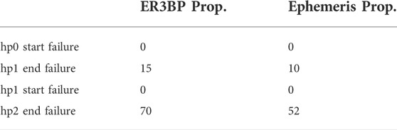
TABLE 1. Number of Safety Violations in the original Sequence Innocenti et al. (2022).

TABLE 2

TABLE 2. Number of Safety Violations with the reallocated Sequence, Innocenti et al. (2022).

TABLE 3

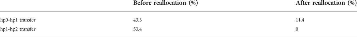
TABLE 3. Random ΔVs in hp0-hp1 and hp1-hp2 Transfers - Safety Violations Innocenti et al. (2022).

In the next example we show the simulation of a new rendezvous attempt performed after one orbit with the chaser not entering the Rendezvous Sphere for the entire orbit period of the Gateway. The ER3BP propagation equations are used.

The rendezvous is performed after a missed firing at hp0. The final chaser position is ρ = (240.0, −6.0, −135.0) km, therefore the relative distance is 275 km. The new hold point sequence and relative times of flight are given by:

• hp0 = (240.0; −6.0; −135.0) km;

• hp1 = (150.0; 0; −75.0) km, TOF = 20 h;

• hp2 = (50.0; 0; −15.0) km, TOF = 20 h;

• hp3 = (20.0; 0; −15.0) km, TOF = 10 h;

• hp4 = (2.0; 0; 0) km, TOF = 10 h;

We have seen previously that the optimization procedure yielding the new sequence and transfer times depends primarily from passive safety and ΔV requirements. With an initial mean anomaly at hp0 equal selected as 100°, because the rendezvous phase must occur for values of MA between [80°, 280°], the total time of flight of the new rendezvous attempt after one orbit must not exceed a half period, or about 75 h. The locations of the new hold points are along lines outside the Rendezvous Sphere.

Supplementary Figure S9 describes the complete attempt in the preferred R-bar V-bar plane as well as the H-bar component. The blue line indicates the free drift path departing from the original hp0, and propagated for one target orbital period under the ER3BP model. The chaser must firstly stop at the new hp0 (it is assumed that the actuator failure is recovered by the time of the second attempt). Then, each subsequent sequence is performed as before, with impulsive maneuvers, and the resulting trajectory, depicted with a black line in the figure, is obtained again with the ER3BP model. The total ΔV of the new rendezvous maneuver is about 10 m/s, with a final mean anomaly of 243°.

6 Near range closed loop guidance approaches

During the final segment of rendezvous, closed loop guidance is necessary to achieve the required precision in relative position and attitude between LAE and the Gateway.

There are many methods to guidance and control design available in the literature. Reference Lian and Tang (2013) uses terminal sliding mode control for instance. A fixed-time glideslope guidance algorithm on a quasi-periodic halo orbit can be found in Lian et al. (2012). Another reference of interest, although limited to LEO, is Mammarella (2016), here the authors use linear optimal regulator control combined with pronav. Hartley and coworkers applied MPC techniques for a rendezvous in a two body problem Hartley et al. (2012). An application of H-infinity control can be found in Franzini et al. (2016), with linearization constraints. Lastly, the new realm of artificial intelligence has begun to show its capabilities as in Tofanelli et al. (2021), among others.

In this paper we refer primarily to work done by Galullo in Galullo (2018). The technique used for closed loop guidance is uses the state dependent Riccati equation method (SDRE), which provides a systematic approach optimal control to a class of non-linear systems. SDRE were studied successfully for variety of applications as described in Cimen (2012) for instance. Space specific applications can be found in Massari and Zazzera (2014) and Tannous et al. (2018).

6.1 Attitude dynamics

During the closed loop part of the rendezvous translation and attitude equations of relative motion are considered. For the relative translation we refer to Subsection 3.2. The relative attitude dynamics are obtained following Ankersen (2011), starting from a body axes reference frame located at the center of mass of each vehicle.

The chaser attitude dynamics are, in standard vector form:

$\mathbb{I}\dot{\mathit{\omega }}+\mathit{\omega }\times \mathbb{I}\mathit{\omega }=\mathbf{N}(35)$

where N is the total applied moment, $\mathbb{I}$ is the inertia matrix and ω is the angular velocity of the non inertial frame. Note that ω can be computed as:

$\mathit{\omega }={\mathit{\omega }}_{c/i}={\mathit{\omega }}_{c/l}+{\mathit{\omega }}_{l/i}$

with ω_c/l the angular velocity of the vehicle with respect to the $\mathcal{L}$ and ω_l/i is the angular velocity of the $\mathcal{L}$ frame with respect to inertial reference.

The kinematics can be described by the usual Euler angles or by quaternions. Based on Ankersen (2011), the following definition was used in this work: $q_1=\cos (\frac{\theta }{2})$, $q_i=e_i\sin (\frac{\theta }{2})$ with i = 2, 3, 4; where $\mathbf{e}={\left[e_2,e_3,e_4\right]}^{\top }$ is the rotation eigenaxis direction and θ is the rotation angle around e. The relationship between quaternions and angular velocity is then:

$\begin{array}{cc}\hfill {\dot{\mathbf{q}}}_{c/l}& =\frac{1}{2}\left[\begin{array}{cc}\hfill 0\hfill & \hfill -{\mathit{\omega }}_{c/l}^{\top }\hfill \\ \hfill {\mathit{\omega }}_{c/l}\hfill & \hfill -{\left[{\mathit{\omega }}_{c/l}\right]}^{\times }\hfill \end{array}\right]{\mathbf{q}}_{c/l}\hfill \\ \hfill & =\frac{1}{2}\mathbf{Q}\left({\mathit{\omega }}_{c/l}\right){\mathbf{q}}_{c/l}\hfill \end{array}(36)$

with q_c/l the quaternion that describes the relative attitude between the body and LVLH frames $\mathcal{C}$ and $\mathcal{L}$, and [⋅]^× denotes the operator that transforms a vector into the associated antisymmetric matrix. The set of differential equations given by Eqs 35, 36 provide the non-linear attitude model of chaser Wie (2008) and Ankersen (2011).

Since there are no viable models for the Gateway’s attitude, we refer to the ISS dynamics, which has a sawtooth profile. The model used consists of an harmonic oscillator described in Eq. 37 below Ankersen (2011).

$\left[\begin{array}{c}\hfill {\dot{\mathbf{q}}}_{t/l}\hfill \\ \hfill {\dot{\mathit{\omega }}}_{t/l}\hfill \end{array}\right]=\left[\begin{array}{cc}\hfill \frac{1}{2}\mathbf{Q}\left({\mathit{\omega }}_{t/l}\right)\hfill & \hfill {\mathbf{0}}_{4\times 3}\hfill \\ \hfill -{\mathbf{K}}_{qt}\hfill & \hfill {\mathbf{0}}_{3\times 3}\hfill \end{array}\right]\left[\begin{array}{c}\hfill {\mathbf{q}}_{t/l}\hfill \\ \hfill {\mathit{\omega }}_{t/l}\hfill \end{array}\right](37)$

For clarity’s sake, the attitude of the target’s body frame with respect to LVLH is q_t/l, with time derivative ${\dot{\mathbf{q}}}_{t/l}$. The angular velocity and acceleration of the target with respect to LVLH frame are ω_t/l and ${\dot{\mathit{\omega }}}_{t/l}$. The time derivative of the quaternion with the angular velocity are related by the matrix Q(⋅), and K_qt is a diagonal matrix containing the eigen frequency for each axis.

The attitude dynamics of relative motion can then be found in body frame as:

${\mathit{\omega }}_{c/t}={\mathit{\omega }}_{c/l}-{\mathbf{R}}_{cl}\left({\mathbf{q}}_{\mathbf{c}∕\mathbf{l}}\right){\mathit{\omega }}_{t/l}(38)$

R_cl(q_c∕l) is the standard transformation matrix between the $\mathcal{L}$ frame and the $\mathcal{C}$ frame.

${\mathbf{R}}_{cl}\left({\mathbf{q}}_{c/l}\right)=\left[\begin{array}{ccc}\hfill 1-2\left(q_3^2+q_4^2\right)\hfill & \hfill 2\left(q_2{q}_3+q_1{q}_4\right)\hfill & \hfill 2\left(q_2{q}_4-q_1{q}_3\right)\hfill \\ \hfill 2\left(q_2{q}_3-q_1{q}_4\right)\hfill & \hfill 1-2\left(q_2^2+q_4^2\right)\hfill & \hfill 2\left(q_3{q}_4+q_1{q}_2\right)\hfill \\ \hfill 2\left(q_2{q}_4+q_1{q}_3\right)\hfill & \hfill 2\left(q_3{q}_4-q_1{q}_2\right)\hfill & \hfill 1-2\left(q_2^2+q_3^2\right)\hfill \end{array}\right](39)$

given the relative angular velocity ω_c/t, we the obtain the derivative of the associated quaternion as: ${\dot{\mathbf{q}}}_{c/t}=\frac{1}{2}\mathbf{Q}({\mathit{\omega }}_{c/t}){\mathbf{q}}_{c/t}$.

6.2 SDRE guidance controller

The structure of the guidance controller follows the general SDRE format, assuming in our case a full state availability for feedback. Using a state dependent coefficient parametrization, the relative motion dynamics assume a linear form in the state space as Cimen (2012):

$\dot{\mathbf{x}}=\mathbf{A}(\mathbf{x})\mathbf{x}+\mathbf{B}(\mathbf{x})\mathbf{u}(40)$

The optimal controller is found by solving a LQR-like full state feedback optimization yielding:

$\begin{array}{c}\hfill \mathbf{u}=-\mathbf{P}\left(\mathbf{x}\right)\mathbf{x}=-\left[\begin{array}{c}\hfill {\mathbf{P}}_0\left(\mathbf{x}\right)+{\mathbf{P}}_{\mathrm{\Omega }}\left(\mathbf{x}\right)\hfill \end{array}\right]\mathbf{x}\end{array}(41)$

where

${\mathbf{P}}_0\left(\mathbf{x}\right)={\bar{\mathbf{R}}}^{-1}\left(\mathbf{x}\right)\mathbf{B}\left(\mathbf{x}\right)\bar{\mathbf{S}}\left(\mathbf{x}\right){\mathbf{P}}_{\mathrm{\Omega }}\left(\mathbf{x}\right)={\bar{\mathbf{R}}}^{-1}\left(\mathbf{x}\right){\mathbf{D}}^T\left(\mathbf{x}\right){\mathbf{W}}_z\left(\mathbf{x}\right)\mathbf{C}\left(\mathbf{x}\right)(42)$

Equation 41 contains two terms: the first P₀ is the gain from the original Riccati solution, while P_Ω depends on additional constraints that may be present on the relative position and velocity during the final phase, in order to satisfy the required safety corridor. They are introduced via SDC parametrization with a weighted fictitious output z Massari et al. (2012), Galullo et al. (2022) given by:

$\mathbf{z}=\mathbf{C}(\mathbf{x})\mathbf{x}+\mathbf{D}(\mathbf{x})\mathbf{u}(43)$

The quadratic performance index that yields Eq. 41 is given by:

$\begin{array}{cc}\hfill H\left(\mathbf{x},\mathbf{u}\right)& =H_0\left(\mathbf{x},\mathbf{u}\right)+H_{\mathrm{\Omega }}\left(\mathbf{x},\mathbf{u}\right)=\hfill \\ \hfill & =\frac{1}{2}{\int }_0^{\infty }\left({\mathbf{x}}^{\top }\mathbf{Q}\left(\mathbf{x}\right)\mathbf{x}+{\mathbf{u}}^{\top }\mathbf{R}\left(\mathbf{x}\right)\mathbf{u}\right)dt+\frac{1}{2}{\int }_0^{\infty }\left({\mathbf{z}}^{\top }{\mathbf{W}}_z\left(\mathbf{x}\right)\mathbf{z}\right)dt\hfill \end{array}(44)$

The specific parametrizations used for our problem and reported in Eq. 40 can be found in Galullo et al. (2022), and Lee et al. (2014).

6.3 Simulation results

In the final part of the rendezvous, the chaser should approach the target from a direction limited by a safety zone defined by collision avoidance requirements. In this work a simpler cone-like final approach corridor is considered as in Dong et al. (2017).

Supplementary Figure S10 depicts an artistic representation of a safety zone, where p is the unit vector of the trajectory direction, and β is the maximum value of the cone angle of the corridor, which is the design parameter.

The validation of the guidance controller described above was performed via simulation using extensive Montecarlo analysis. An example of guidance performance is presented next for an approach at the aposelene. The equations of relative motion are those based on the CR3BP normalized as in Koon et al. (2011), and accurate enough for the closed loop analysis.

Supplementary Figure S11 shows simulation initial conditions. The attitude dynamics of the Gateway is limited to a maximum amplitude of 5° with eigen-frequency equal to k_qt = 0.1571 rad⋅s⁻¹ Fehse (2003). The chaser is modelled as a cylinder with inertia matrix $\mathbb{I}$ = diag(0.0011, 0.0006, 0.0006) kg ⋅ km² Bucchioni (2021). The direction vector of the approaching cone is ${\left[\mathbf{p}\right]}_{\mathcal{T}}={\left[-1,0,0\right]}^{\top }$ and the maximum cone angle is set to β = 25°.

The terminal conditions chosen relative position and relative velocity were ρ ≤ 1 m, and $\dot{\rho }\le$ 0.03 m/s (note that for ESA’s ATV mission concept the constraints were 20 m in relative position, and 0.01 m/s for relative velocity Fehse (2003)).

The SDRE controller was evaluated with a limited simulation campaign for six different relative distances ρ = 5, 8, 11, 14, 17, 20 Km, for which 20 random uniformly distributed points were selected. The performance analysis was based on normalized values of position error, error rate and amount of control, over the time of flight period.

$I{e}_{\rho }={\int }_0^{t_{of}}\Vert {\mathbf{e}}_{\rho }\left(t\right)\Vert dtI{e}_{\dot{\rho }}={\int }_0^{t_{of}}\Vert {\mathbf{e}}_{\dot{\rho }}\left(t\right)\Vert dt{\delta }_v={\int }_0^{t_{of}}\Vert {\mathbf{u}}_{\Vert }dt(45)$

The errors between true and estimated position, velocity and equivalent propellant usage are indicated by e_ρ(t), ${\mathbf{e}}_{\dot{\rho }}(t)$ and δ_v respectively.

Supplementary Figure S12 presents a phase plane in the V-bar and R-bar directions of the relative position between chase and Gateway (located at the center). Time of flight and control effort versus initial relative distance are shown in Supplementary Figures S13, S14.

It is clear from Supplementary Figures S13, S14 that the total effort δ_v and time of flight t_of increase with the distance, as expected. The linearity in Supplementary Figure S13 underlines the validity of the CR3BP model at the aposelene for preliminary closed loop guidance design.

7 ROSSONERO

All the results presented in the paper were obtained using a simulation software developed ad hoc to provide the mission designer with a variety of tools for the analysis and design of a rendezvous manoeuvre, which satisfies a set of safety requirements.

ROSSONERO (Rendezvous Operations Simulation Software on Near Rectilinear Orbit) is a simulation framework for the design of phasing and rendezvous maneuvers between an active chaser spacecraft and a passive target spacecraft in highly non-Keplerian orbits in which the third body perturbation can not be neglected. It was developed with a particular focus on the rendezvous and proximity operations in the Earth—Moon L2 location of the upcoming Lunar Orbital Platform Gateway. However, the tool is structured so that it can handle different orbit types, different spacecraft architectures and different three-body problem scenarios. The software simulates the full 6-DOF relative dynamics and control in a combined MATLAB/Simulink environment.

The absolute translational motion of chaser and target spacecraft are modelled using the ER3BP, with respect to a Moon-centered rotating frame and then used to compute relative position and velocity in a target-centered LVLH frame (see Figure 3).

ROSSONERO has three main components: the graphical user interface (GUI), a set of MATLAB scripts to define chaser’s geometry, docking/berthing ports positions, sensors and actuators positions, guidance parameters, etc., and several Simulink models for dynamics simulation.

For the availability of the software, and additional information the reader can contact the authors or refer to Innocenti et al. (2021).

8 Conclusion

The paper presents an overview of the research carried out by the authors under ESA contract described in the funding section. The work deals with several dynamics and control issues arising in the design of a rendezvous trajectory between a chaser spacecraft and a passive Gateway space station. The assumed location of the Gateway required the dynamic analysis to be performed within a non-Keplerian three body problem setting, for which scientific and technological aspects were not exhaustively available in the literature. Although the scope of the paper is to provide a general overview, additional technical details can be found in the appropriate references by the authors.

Data availability statement

The original contributions presented in the study are included in the article/Supplementary Materials, further inquiries can be directed to the corresponding author.

Author contributions

MI and GF contributed to the initial concept and design of the study. MI and GB further defined improvements in the dynamic model and theoretical framework for the long range approach. Failure analysis was carried out by MI, GB, and FO closed loop short range guidance was studied by MI, GF, and MG. Computational aspects and simulations were carried out primarily by GF, GB, FO, and MG. The data and scenarios were discussed by MI, AC, and MC within the funding requirements. The manuscript was written by MI with contributions by all authors who read, and approved the submitted version.

Funding

This work was partially supported by the European Space Agency under contract No. 000121575/17/NL/hh and CCN1, CCN2, CCN3 extensions. The view expressed herein can in no way be taken to reflect the official opinion of the European Space Agency.

Acknowledgments

The authors wish to acknowledge the contribution of several graduate students at the University of Pisa for the generation of some of the numerical data base used in the work. The content of this manuscript has been presented IN PART at the following conferences: AIAA - SCITECH 2021, AIAA - SCITECH 2022 and ESA - ICATT 2021 of which the authors retain the copyright.

Conflict of interest

Author MG was employed by the company Leonardo Underwater Systems.

The remaining authors declare that the research was conducted in the absence of any commercial or financial relationships that could be construed as a potential conflict of interest.

Publisher’s note

All claims expressed in this article are solely those of the authors and do not necessarily represent those of their affiliated organizations, or those of the publisher, the editors and the reviewers. Any product that may be evaluated in this article, or claim that may be made by its manufacturer, is not guaranteed or endorsed by the publisher.

Supplementary material

The Supplementary Material for this article can be found online at: https://www.frontiersin.org/articles/10.3389/frspt.2022.929179/full#supplementary-material

SUPPLEMENTARY FIGURE S1 | Control Allocation Performance vs. PWM Duration for a sample Rendezvous.

SUPPLEMENTARY FIGURE S2 | Typical Safety Boundaries Bucchioni (2021).

SUPPLEMENTARY FIGURE S3 | Nominal Rendezvous Sequence and Safety Areas.

SUPPLEMENTARY FIGURE S4 | Nominal Rendezvous Trajectory - ER3BP vs. Ephemeris Models.

SUPPLEMENTARY FIGURE S5 | Scheme of assumed Failures during Rendezvous.

SUPPLEMENTARY FIGURE S6 | Definition of α_collision.

SUPPLEMENTARY FIGURE S7 | Graph for the Selection of the Optimal Sequence of hold-points.

SUPPLEMENTARY FIGURE S8 | Hold Points Reallocation using Eq. 34.

SUPPLEMENTARY FIGURE S9 | New Rendezvous Sequence after missed start firing at hp0) Innocenti et al. (2022).

SUPPLEMENTARY FIGURE S10 | Approaching Cone Constraint.

SUPPLEMENTARY FIGURE S11 | Initial Conditions for close Range Rendezvous.

SUPPLEMENTARY FIGURE S12 | LAE-Gateway Relative Position, Aposelene Approach.

SUPPLEMENTARY FIGURE S13 | Time of Flight versus Distance.

SUPPLEMENTARY FIGURE S14 | Control Effort versus Distance.

References

Alfriend, K. T., and Yan, H. (2005). Evaluation and comparison of relative motion theories. J. Guid. Control, Dyn. 28, 254–261. doi:10.2514/1.6691

CrossRef Full Text | Google Scholar

Ankersen, F. (2011). Guidance, navigation, control and relative dynamics for spacecraft proximity maneuvers. Ph.D. thesis. Aalborg, Denmark: Aalborg University, Department of Electronic Systems.

Google Scholar

Blazquez, E., Beauregard, L., and Lizy-Destrez, S. (2018a). “Optimized transfers between earth-moon invariant manifolds,” in 7th ICATT conference (ESA), 1–9.

Google Scholar

Blazquez, E., Beauregard, L., and Lizy-Destrez, S. (2018b). “Safe natural far rendezvous approaches for cislunar near rectilinear halo orbits in the ephemeris model,” in Proceedings of the 7th ICATT conference.

Google Scholar

Breger, L., and How, J. P. (2008). Safe trajectories for autonomous rendezvous of spacecraft. J. Guid. Control Dyn. 31, 1478–1489. doi:10.2514/1.29590

CrossRef Full Text | Google Scholar

Bucchioni, G., and Innocenti, M. (2021a). Phasing maneuver analysis from a low lunar orbit to a near rectilinear halo orbit. Aerosp. (Basel). 8, 70–26. doi:10.3390/aerospace8030070

CrossRef Full Text | Google Scholar

Bucchioni, G., and Innocenti, M. (2021b). Rendezvous in cis-lunar space near rectilinear halo orbit: Dynamics and control issues. Aerosp. (Basel). 8 (3), 68–38. doi:10.3390/aerospace8030068

CrossRef Full Text | Google Scholar

Bucchioni, G. (2021). PhD thesis: Guidance and control for phasing, rendezvous and docking in the three body lunar space. Pisa, Italy: University of Pisa.

Google Scholar

Bucci, L., Lavagna, M., and Renk, F. (2017). Relative dynamics analysis and rendezvous techniques for lunar near rectilinear halo orbits. Proc. 68th Int. Astronaut. Congr. (IAC 2017) 12, 7645–7654.

Google Scholar

Cimen, T. (2012). Survey of state-dependent riccati equation in nonlinear optimal feedback control synthesis. J. Guid. Control, Dyn. 35, 1025–1047. doi:10.2514/1.55821

CrossRef Full Text | Google Scholar

Clohessy, W. H., and Wiltshire, R. S. (1960). Terminal guidance system for satellite rendezvous. J. Aerosp. Sci. 27, 653–658. doi:10.2514/8.8704

CrossRef Full Text | Google Scholar

Colagrossi, A., and Lavagna, M. (2018). Dynamical analysis of rendezvous and docking with very large space infrastructures in non-keplerian orbits. CEAS Space J. 10, 87–99. doi:10.1007/s12567-017-0174-4

CrossRef Full Text | Google Scholar

De Benedetti, M., Bucchioni, G., D’Onofrio, F., and Innocenti, M. (2022). Fully safe rendezvous strategy in cis-lunar space: Passive and active collision avoidance. J. Astronautical Sci. In press.

CrossRef Full Text | Google Scholar

Dong, H., Hu, Q., and Akella, M. R. (2017). Dual-quaternion-based spacecraft autonomous rendezvous and docking under six-degree-of-freedom motion constraints. J. Guid. Control, Dyn. 41, 1150–1162. doi:10.2514/1.G003094

CrossRef Full Text | Google Scholar

Fehse, W. (2003). Automated rendezvous and docking of spacecraft. New York: Cambridge University Press.

Google Scholar

Franzini, G., and Innocenti, M. (2019). Relative motion dynamics in the restricted three-body problem. J. Spacecr. Rockets 56, 1322–1337. doi:10.2514/1.A34390

CrossRef Full Text | Google Scholar

Franzini, G., and Innocenti, M. (2017). “Relative motion equations in the local-vertical local-horizon frame for rendezvous in lunar orbits,” in Proceedings of the 2017 AAS/AIAA astrodynamics specialist conference (Stevenson, WA, USA), 17–641. Paper AAS.

Google Scholar

Franzini, G., Pollini, L., and Innocenti, M. (2016). “H-infinity controller design for spacecraft terminal rendezvous on elliptic orbits using differential game theory,” in American control conference (ACC), 2016 (IEEE), 7438–7443.

CrossRef Full Text | Google Scholar

Galullo, M., Bucchioni, G., Franzini, G., and Innocenti, M. (2022). Closed loop guidance during close range rendezvous in a three body problem. J. Astronaut. Sci. 69, 28–50. doi:10.1007/s40295-021-00289-6

CrossRef Full Text | Google Scholar

Galullo, M. (2018). MS thesis: SDRE guidance and navigation for spacecraft relative motion. Pisa, Italy: University of Pisa.

Google Scholar

Gomez, G., Llibre, J., Martinez, R., and Simo’, C. (2001). Dynamics and mission design near libration points. Vol I. Fundamentals: The Case of collinear libration points. World Scientific Monograph Series: Mathematics.

Google Scholar

Gurfil, P., and Seidelmann, P. K. (2016). Celestial mechanics and astrodynamics: Theory and practice. Springer.

Google Scholar

Hartley, E. N., Trodden, P. A., Richards, A. G., and Maciejowski, J. M. (2012). Model predictive control system design and implementation for spacecraft rendezvous. Control Eng. Pract. 20, 695–713. doi:10.1016/j.conengprac.2012.03.009

CrossRef Full Text | Google Scholar

Howell, K. (2001). Families of orbits in the vicinity of the collinear libration points. J. Astronaut. Sci. 49, 107–125. doi:10.1007/BF03546339

CrossRef Full Text | Google Scholar

Innocenti, M., Bucchioni, G., and D’Onofrio, F. (2020). Simulation tool for rendezvous and docking in high elliptical orbits with third body perturbation: Final report. ESA Contract No. 4000121575/17/NL/CRS/hh-CCN2.

Google Scholar

Innocenti, M., Bucchioni, G., and D’Onofrio, F. (2021). Simulation tool for rendezvous and docking in high elliptical orbits with third body perturbation: Final report. ESA Contract No. 4000121575/17/NL/CRS/hh-CCN3.

Google Scholar

Innocenti, M., and Bucchioni, G. (2019). Simulation tool for rendezvous and docking in high elliptical orbits with third body perturbation: Final report. ESA Contract No. 4000121575/17/NL/CRS/hh-CCN1.

Google Scholar

Innocenti, M., D’Onofrio, F., and Bucchioni, G. (2022). “Failure mitigation during rendezvous in cislunar orbit,” in Scitech 2022 (AIAA American Institute of Aeronautics and Astronautics), 1–19. AIAA 2022-0861. doi:10.2514/6.2022-0861

CrossRef Full Text | Google Scholar

Innocenti, M., and Franzini, G. (2018). Simulation tool for rendezvous and docking in high elliptical orbits with third body perturbation: Final report. ESA Contract No. 4000121575/17/NL/CRS/hh.

Google Scholar

Koon, W. S., Lo, M. W., Marsden, J. E., and Ross, S. D. (2011). Dynamical systems, the three-body problem and space mission design. Los Angeles, CA: Marsden Books.

Google Scholar

Landgraf, M. (2019). Heracles: An esa-jaxa-csa joint study on returning to the moon. 50th Lunar Planet. Sci. Conf. 1, 1–2.

Google Scholar

Lee, D., Bang, H., Butcher, E. A., and Sanyal, A. K. (2014). Kinematically coupled relative spacecraft motion control using the state-dependent riccati equation method. J. Aerosp. Eng. 28, 1–13. doi:10.1061/(ASCE)AS.1943-5525.0000436

CrossRef Full Text | Google Scholar

Lian, Y., Meng, Y., Tang, G., and Liu, L. (2012). Constant-thrust glideslope guidance algorithm for time-fixed rendezvous in real halo orbit. Acta Astronaut. 79, 241–252. doi:10.1016/j.actaastro.2012.04.049

CrossRef Full Text | Google Scholar

Lian, Y., and Tang, G. (2013). Libration point orbit rendezvous using pwpf modulated terminal sliding mode control. Adv. Space Res. 52, 2156–2167. doi:10.1016/j.asr.2013.08.034

CrossRef Full Text | Google Scholar

Lizy-Destrez, S., Beauregard, L., Blazquez, E., Campolo, A., Manglativi, S., and Quet, V. (2019). Rendezvous strategies in the vicinity of earth-moon Lagrangian points. Front. Astron. Space Sci. 5, 1–19. doi:10.3389/fspas.2018.00045

CrossRef Full Text | Google Scholar

Luo, Y., Liang, L. B., Wang, H., and Tang, G. J. (2014). Quantitative performance for spacecraft rendezvous trajectory safety. J. Guid. Control, Dyn. 34, 1264–1269. doi:10.2514/1.52041

CrossRef Full Text | Google Scholar

Luo, Y., Liang, Z., and Tang, G. (2013). Safety-optimal linearized impulsive rendezvous with trajectory uncertainties. J. Aerosp. Eng. 27, 431–438. doi:10.1061/(asce)as.1943-5525.0000366

CrossRef Full Text | Google Scholar

Mammarella, M. (2016). Guidance and control algorithms for space rendezvous and docking maneuvers. Astrodyn. Spec. Conf. 8.

Google Scholar

Massari, M., and Zazzera, F. (2014). Application of sdre technique to orbital and attitude control of spacecraft formation flying. Acta Astronaut. 94, 409–420. doi:10.1016/j.actaastro.2013.02.001

CrossRef Full Text | Google Scholar

Massari, M., Zazzera, F., and Canavesi, S. (2012). Nonlinear control of formation flying with state constraints. J. Guid. Control, Dyn. 35, 1919–1925. doi:10.2514/1.55590

CrossRef Full Text | Google Scholar

May, Z. D., Qu, M., and Merrill, R. (2020). “Enabling global lunar access for human landing systems staged at earth-moon l2 southern near rectilinear halo and butterfly orbits,” in Scitech 2020 (AIAA (American Institute of Aeronautics and Astronautics), 1–21. AIAA 2020-0962. doi:10.2514/6.2020-0962

CrossRef Full Text | Google Scholar

NASA (2015). Nasa’s lunar exploration program overview.

Google Scholar

Renk, F., Landgraf, M., and Bucci, L. (2018). “Refined mission analysis for heracles - a robotic lunar surface sample return mission utilizing human infrastructure,” in 2018 AAS/AIAA astrodynamics specialist conference (Snowbird, UT, USA, 18–344.

Google Scholar

Renk, F., Landgraf, M., and Roedelsperger, M. (2017). “Operational aspects and low thrust transfers for human-robotic exploration architectures in the earth-moon system and beyond,” in Proceedings of the 2017 AAS/AIAA astrodynamics specialist conference (Stevenson, WA, USA.

Google Scholar

Shang, H., Wang, S., and Wu, W. (2015). Design and optimization of low-thrust orbital phasing maneuver. Aerosp. Sci. Technol. 42, 365–375. doi:10.1016/j.ast.2015.02.003

CrossRef Full Text | Google Scholar

Tannous, M., Franzini, G., and Wu, M. I. (2018). “State-dependent riccati equation control for spacecraft formation flying in the circular restricted three-body problem,” in Astrodynamics specialist conference (Springfield, VA: AAS AIAA), 162, 2603–2617.

Google Scholar

Tofanelli, G., Bucchioni, G., and Innocenti, M. (2021). “Closed-loop neural control for the final phase of a cislunar rendezvous,” in Proceedings of the 2021 astrodynamics specialist conference (Springfield, VA: AAS-AIAA). AAS-21-630.

Google Scholar

Topputo, F. (2015). Fast numerical approximation of invariant manifolds in the circular restricted three-body problem, 1–18.

Google Scholar

Tschauner, J., and Hempel, P. (1965). Rendezvous zu einem in elliptischer bahn umlaufenden ziel. Astronaut. Acta 11, 104–109.

Google Scholar

Ueda, S., Murakami, N., and Ikenaga, T. (2017). “A study on rendezvous trajectory design using invariant manifolds of cislunar orbits,” in SCITECH 2017, AIAA guidance, navigation, and control conference (Springfield, VA: Grapevine TX).

Google Scholar

Whitley, R., and Martinez, R. (2018). “Earth-moon near rectilinear halo and butterfly orbits for lunar surface exploration,” in AAS/AIAA astrodynamics specialist conference (American Astronautical Society), 1–20.

Google Scholar

Whitley, R., and martinez, R. (2016). “Options for staging orbits in cislunar space,” in 2016 IEEE aerospace conference (IEEE), 1–9.

CrossRef Full Text | Google Scholar

Wie, B. (2008). Space vehicle dynamics and control. 2 edn. American Institute of Aeronautics and Astronautics.

Google Scholar

Woffinden, D. C. (2007). Relative angles-only navigation and pose estimation for autonomous orbital rendezvous. J. Guid. Control Dyn. 30, 1455–1469. doi:10.2514/1.28216

CrossRef Full Text | Google Scholar