Instabilities in a Spherical Liquid Drop

We examine cases of stationary vortices that can appear inside spherical liquid drops in microgravity conditions. The first case is that of an incompressible external flow of uniform speed at infinity, leading the liquid in the drop by friction to form a Hill vortex. In the second case, the external fluid does not interact by friction with the liquid, but the drop is subjected to an axial temperature gradient causing a variation in surface tension. This time it is the induced movement which entrains the internal liquid. Note that the two situations can lead to the same Hill vortex. Combined effects are envisioned. We are also interested in the time factor in these phenomena.

1 Introduction

The drops of the sprays undergo various actions depending on their origin and the resulting physical situation in which they are found, such as watering spray, medical spray, automotive engine injector, rocket engine injector, etc. Their modeling includes on the one hand the examination on the scale of each individual drop, and on the other hand the study of the spray itself on a larger scale, as a constituent of a multiphase flow which is most often liquid-gas. Individual drop is often considered to be spherical. This is the case with small drops where capillary efforts are decisive for the establishment of sphericity. This simplicity of geometric shape is called into question in the case of large drops and as soon as they are subjected to significant forces of aerodynamic origin for example.¹

For the sake of simplicity, we try during theoretical research to keep the spherical shape as long if possible.

The microgravity can be considered as a factor favorable to the spherical shape of the drops of average size which can allow experimental observation.

Finally, the study is also interested in applications to launchers. This dual fundamental/applied aspect makes the study of sprays a reason of choice recommended by CNES within the framework of Material Sciences.²

The exchanges between the individual drop and its gaseous environment are obviously different depending on whether there is evaporation-condensation or not. They concern the masses of the constituents, the momentum, and the energy. Each phase involved also undergoes motions and transfer phenomena.

For the flow of the spray itself, it is often necessary to model what happens inside the individual drops. The most classic is to characterize the latter by their radius, their mass, their temperature and their speed. The distribution in diameter and speed of the drops will always remain the essential element.

Nevertheless, it may be interesting to take care of the internal motions of medium-sized drops because these act on the exchanges at their surface. This is the problem that is proposed in this article, where we will therefore have to simultaneously study the external and internal flows of individual drops.

We have retained here the case of spherical liquid drops subjected either to a uniform external gas flow, or to a thermal gradient in an axial direction. We will see that Hill’s vortex modeling is an interesting solution for interior flows.

One of the major problems is that of the connection between the flow inside the drop-limiting sphere and the flow of the outside fluid.

Indeed, if we assume a perfect fluid on the outside, we can logically be led to admit perfect sliding conditions for this fluid at the level of the surface of the drop. But then how to admit that there is entrainment of the internal liquid in the drop by the external fluid?

The problem of the forces exerted on the drop by the external fluid is also posed regarding their resultant which is found to be zero! This constitutes the famous Dalembert paradox. We are then invited to consider the viscosity of the external fluid, at least in the close vicinity of the sphere, which leads to Stokes’ theory in the case of the rigid sphere. The results must also be modified to consider a liquid sphere. And in the presence of evaporation-condensation of the liquid it is even more complicated!

Finally, we know that for many linear problems one can superimpose elementary solutions. We will do this whenever possible, considering the nature of the fluids and the areas of validity that are the interior and exterior of the drop.

The origin of our study is related to the problem of combustion instabilities in rocket engines: It is established that the evaporation of droplets during combustion is the cause of amplification of HF vibrations generated by the engine (This model is mentioned in the appendix.). A feeded drop model was developed to represent the evaporating spray being. This model results from an improvement of that of Heidmann which did not consider the internal irreversibilities of the drop in evaporation. But if this model, with spherical symmetry, is well adapted to the velocity nodes (pressure anti-nodes) of standing sound waves, it is not suitable for the other zones of these waves presenting simultaneous pressure and velocity oscillations. These speed oscillations actually generate a break in the spherical symmetry, the consequences of which need to be analyzed.

2 Spherical Liquid Drop Subjected to a Uniform External Flow far away

Hill’s vortex is used to model the flow within a spherical liquid drop in the presence of relative external flow (Abramzon and Sirignano, 1989).

This vortex is a special case of a stationary motion of revolution of an incompressible inviscid fluid (Lamb, 1945). It is a rotational motion inside a sphere behaving with an irrotational external flow, so that by choosing suitably the multiplicative constant α of the stream function, the speeds of the two flows are identical to the surface of the sphere (Germain, 1986).

We first recall the equations of the fluid flow outside the sphere of radius R, and we will then determine the velocity field of the compatible steady liquid flow³ inside this same sphere (Prud’homme, 2012).

The stationary flow of a perfect fluid inside a sphere of radius R and the flow around this sphere are characteristic examples, shown in Figure 1.

FIGURE 1

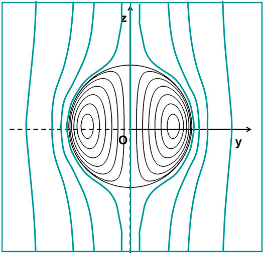
FIGURE 1. Liquid drop in the presence of an infinitely uniform flow: shape of the streamlines of the external and internal flows in a plane passing through the axis of symmetry.

2.1 Incompressible Fluids in Spherical Coordinates

2.1.1 Understanding the Coordinate System

The quantities $\mathrm{r},\theta ,\varphi$, are the spherical coordinates, represented in Figure 2.

FIGURE 2

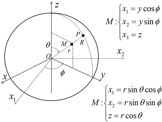
FIGURE 2. Definition of the spherical coordinates and representation of a sphere of radius R. The current point M can be inside or outside the considered sphere. p is the point of the half-line OM located at the surface of the sphere.

In the case of a symmetry around the axis Oz, one works in the plane $\varphi =const.$ of Figure 2 since the motion is independent of this angle. The basic unit vectors can be defined there.

2.1.2 Continuity Equation

The continuity equation of an incompressible fluid is written in vectorial notations: $\overrightarrow{\mathit{\nabla }}·\overline{\mathrm{v}}=0$ In expanded form, this gives:

$\frac{1}{r^2}\frac{\partial }{\partial r}\left(r^2{v}_r\right)+\frac{1}{r\mathit{sin}\theta }\frac{\partial }{\partial \theta }\left(\mathit{sin}\theta v_{\theta }\right)+\frac{1}{r\mathit{sin}\theta }\frac{\partial v_{\varphi }}{\partial \varphi }=0[1]$

In the case of a symmetry of axis Oz, the motion is identical in each plane containing this axis.

The values of the various quantities of the fluid no longer depend on the angle $\varphi$. The continuity equation is therefore reduced to: $\frac{1}{r^2}\frac{\partial }{\partial r}\left(r^2{v}_r\right)+\frac{1}{r\mathit{sin}\theta }\frac{\partial }{\partial \theta }\left(\mathit{sin}\theta v_{\theta }\right)=0$, and we can then define the velocity field from the stream function $\Psi$ as follows:

$v_r=-\frac{1}{r\mathit{sin}\theta }\frac{\partial \psi }{\partial \theta },v_{\theta }=\frac{1}{r\mathit{sin}\theta }\frac{\partial \psi }{\partial r},v_{\varphi }=0[2]$

2.1.3 Expressions of the Stream Function in the Presence of a Sphere

We consider two kinds of flows: a flow irrotational (e) outside the sphere of radius R, and a rotational flow 1) with vorticity $\omega$ inside the sphere. The flows are connected at any point of their spherical border.

Regarding the vorticity, zero on the outside, it is shown that we have $\omega =5{\alpha }_{i}y$ by virtue of the law of transport of the vortex vector $\overrightarrow{\mathit{\omega }}$ into the interior fluid.

In the spherical coordinate system described above, we gets: $r^2=y^2+z^2$.

The stream functions ${\psi }_e$ and ${\psi }_i$ around and inside the sphere of radius R, are expressed as follows⁴:

$\begin{array}{l}\{\begin{array}{l}{\psi }_e={\alpha }_e{y}^2\left(1-\frac{R^3}{r^3}\right),\mathrm{with}{\alpha }_e=V_0/2\mathrm{for}r\ge R,\mathrm{and}\\ {\psi }_i={\alpha }_i{y}^2\left(R^2-r^2\right),\mathrm{with}{\alpha }_i=-3V_0/4R^2\mathrm{for}r\le R\end{array}\\ \end{array}[3]$

therefore:

$\begin{array}{l}\{\begin{array}{l}{\psi }_e=\frac{V_0}{2}{y}^2\left(1-\frac{R^3}{r^3}\right)\mathrm{for}\mathrm{r}\ge R,\mathrm{and}\\ {\psi }_{\mathrm{i}}=-\frac{3V_{\mathrm{o}}}{4}{y}^2\left(1-\frac{r^2}{R^2}\right)\mathrm{for}r\le R\end{array}\\ \end{array}[4]$

In the problem of motion around a stationary sphere of radius R, the velocity $V_0$ is the one at infinity of the external flow: $V_0=U_{\infty }$.

The calculations carried out with the stream function are summarized in Table 1. Theys are explicited hereafter.

TABLE 1

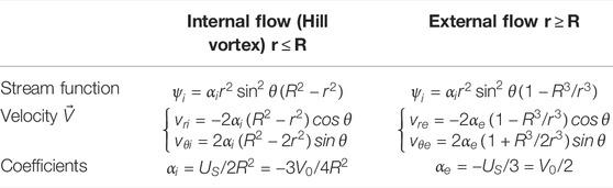
TABLE 1. Correspondence between the coefficients for an external flow coming from the negative x with the velocity modulus $U_{\infty }$. The quantity $U_S$ is the speed at the surface of the sphere at z = 0. This table incorporates the results of Section 2.

2.2 Flow Outside the Sphere

The steady flow of inviscid fluid outside the sphere is an irrotational flow. Its stream function (Figure 3) is (index e for exterior):

${\psi }_e={\alpha }_e{r}^{2}si{n}^2\theta \left(1-\frac{R^3}{r^3}\right),r\ge R,{\alpha }_e=\frac{U_{\infty }}{2}[5]$

FIGURE 3

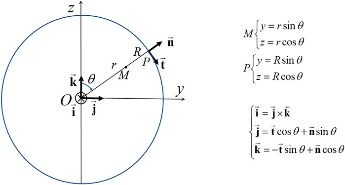
FIGURE 3. Definition of the coordinates in the y0z plane containing the axis of symmetry Oz. At the point p of the surface of the sphere of radius R, we define the unit vectors $\overrightarrow{t}$ tangent and $\overrightarrow{n}$ normal to the great circle considered. These vectors correspond to the base vectors $\left({\overrightarrow{\mathrm{e}}}_{\mathrm{\theta }},{\overrightarrow{\mathrm{e}}}_{\mathrm{r}}\right)$ at the point considered.

The components of the velocity vector are:

$v_{re}=-2{\alpha }_e\left(1-R^3/r^3\right)cos\theta ,v_{\theta e}=2{\alpha }_e\left(1+R^3/2r^3\right)sin\theta [6]$

Its streamlines are represented in Figure 4 with:

$\overline{z}=z/R,\overline{y}=y/R,{\overline{\psi }}_e=2{\psi }_e/U_{\infty }{R}^2[7]$

FIGURE 4

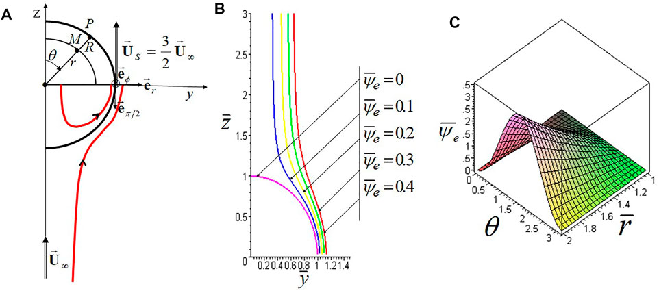
FIGURE 4. (A) Inner and outer streamlines, speed vectors ${\overrightarrow{U}}_{\infty }$ at infinity and ${\overrightarrow{U}}_S$ maximum at the surface. (B) Streamlines of the flow outside the sphere in the upper quarter plane passing through the axis. $\overline{z}=\overline{z}\left(\overline{y}\right)$, for different values of the reduced stream function ${\overline{\psi }}_e=2{\psi }_e/U_{\infty }{R}^2$. (C) Stream function as a function of spherical coordinates $\theta$ and reduced radius $\overline{r}$.

Maximum velocity:

Let us call $U_S$ the value of the speed in $z=0$, $y=R$, which corresponds to $r=R$, $\theta =\pi /2$. We find: $U_{Si}=U_{zi}=2{\alpha }_i{R}^2$, $U_{yi}=0$. If we want $U_S$ to be positive, then we have $\alpha$ to be positive. We then have: ${\alpha }_i=U_S/2R^2$ and the stream function is written: $\frac{U_S}{2R^2}{r}^{2}si{n}^2\theta \left(R^2-r^2\right)$ ${\text{U}}_{\text{S}}$ is the maximum value of $U$ at the surface of the sphere.

The velocity vectors of this flow and of the internal flow will be identical at any point on the surface of the sphere if the speed at infinity is suitably chosen: $U_{re}\left(\infty \right)=-U_{re}\left(-\infty \right)=U_{\infty }$.

2.3 Flow Inside the Sphere

2.3.1 Hill Vortex

The stream function of the form:

$r\le R,{\psi }_i={\alpha }_i{r}^{2}si{n}^2\theta \left(R^2-r^2\right)[8]$

Corresponds to an internal rotational flow (ref. 4).

Knowing the stream function of the internal flow, we find the following radial and angular components of the velocity vector:

$v_{ri}=-2{\alpha }_i\left(R^2-r^2\right)cos\theta ,v_{\theta i}=2{\alpha }_i\left(R^2-r^2\right)sin\theta [9]$

The results are shown in Figure 5.

FIGURE 5

FIGURE 5. (A) Streamlines calculated in the upper quarter plane passing through the axis. $\overline{z}=\overline{z}\left(\overline{y}\right)$, $\overline{y}=y/R$, $\overline{z}=z/R$ for multiple values of ${\overline{\psi }}_{i}4{\psi }_i/{\alpha }_i{R}^4$, ${\overline{z}}_M\left(\overline{y}\right)$. Corresponds to the geometrical locus of the points of contact of the straight lines issued from O and tangents to the streamlines. It is a quarter circle of radius $R\sqrt{2}/2$. The curve ${\overline{z}}_U\left(\overline{y}\right)$ is the geometrical locus of the points where the speed is minimum. (B) Stream function as a function of spherical coordinates $\theta$, $\overline{r}$.

Each value of the stream function corresponds to a toric surface. The limit value ${\overline{\psi }}_i=0$ is the sphere itself.

The velocity vectors of the external flow are identical to those of the Hill vortex at any point on the surface of the sphere if the constants ${\alpha }_i$ and ${\alpha }_e$ are chosen suitably and in relation to the speed at infinity $U_{\infty }$ [one has: $v_{re}\left(\infty \right)=-v_{re}\left(-\infty \right)=U_{\infty }$].

One finds in this case:

${\alpha }_i=3U_{\infty }/4R^2,{\alpha }_e=-U_{\infty }/2[10]$

Let us call $U_S$ the value of the maximum speed at the surface of the sphere, which occurs in $y=R,z=0$, which corresponds to: $\theta =\pi /2$. We find: $U_{Si}=2{\alpha }_i{R}^2$. If you want $U_S$ to be positive, then you have ${\alpha }_i$ to be positive. We then have: ${\alpha }_i=U_S/2R^2$ and the stream function is written:

${\psi }_i=\frac{U_S}{2}{r}^2{\sin }^2\theta \left(R^2-r^2\right)[11]$

We therefore know how to determine the velocity field and the stream surfaces of the flows internal and external to the sphere (ref. iii). It has been shown that then the flows are compatible if ${\alpha }_i=3U_{\infty }/4R^2$. The maximum speed at the surface of the sphere could then be determined.

2.3.2 Remark About Viscous Fluid Vortex

The balance equation of the vortex vector in incompressible viscous fluid is written:

$\partial \overrightarrow{\mathbf{\omega }}/\partial t+\overrightarrow{\nabla }\times \left(\overrightarrow{\mathbf{\omega }}\times \overrightarrow{v}\right)=\nu \mathrm{\Delta }\overrightarrow{\mathbf{\omega }}[12]$

with, in spherical coordinates:

$\omega =\frac{1}{2r}\left[\frac{\partial \left(r{v}_{\theta }\right)}{\partial r}-\frac{\partial v_r}{\partial \theta }\right]{\overrightarrow{\mathit{e}}}_{\varphi }$

In the case of the flow inside the sphere, we find without difficulty for the Hill vortex:

${\overrightarrow{\mathit{\omega }}}_i=-5{\alpha }_{i}rsin\theta {\overrightarrow{e}}_{\varphi }.$

The intensity ${\omega }_i$ of the vortex vector is proportional to the distance $y=rsin\theta$ from the axis of symmetry. The second term of the vortex vector balance is calculated as follows.

We set: $\overrightarrow{\mathit{A}}=\overrightarrow{\nabla }\times \overrightarrow{\mathbf{\omega }}$ and we get:

$A_r=10{\alpha }_{i}rsi{n}^2\theta \left(R^2-2r^2\right),A_{\theta }=10{\alpha }_{i}rsin\theta cos\theta \left(R^2-r^2\right)$

We then find: $\overrightarrow{\mathit{\nabla }}\times \overrightarrow{\mathit{{\rm A}}}=\overrightarrow{\mathit{\nabla }}\times \left(\overrightarrow{\mathit{\nabla }}\times \overrightarrow{\mathit{\omega }}\right)=\frac{1}{2r}\left[\frac{\partial \left(r{A}_{\theta }\right)}{\partial r}-\frac{\partial A_r}{\partial \theta }\right]{\overrightarrow{\mathit{e}}}_{\varphi }=\overrightarrow{\mathbf{0}}$ In steady flow: $\frac{\partial \overrightarrow{\omega }}{\partial t}=\overrightarrow{\mathbf{0}}$. It follows that the term of the second member of the vortex balance Eq. (12), $\nu \Delta \overrightarrow{\mathbf{\omega }}$ is also zero.

The consequence is that Hill’s vortex, a solution of perfect fluid, is also a solution of the equations of viscous fluids.

In the case of external flow, we obviously have ${\overrightarrow{\mathit{\omega }}}_e=\overrightarrow{\mathbf{0}}$ since the flow is irrotational.

3 Flows of a Spherical Liquid Drop Subjected to an Axial Thermal Gradient

3.1 Presentation of the Problem

The effect of an axial temperature field imposed on the internal motions of a liquid spherical drop has been studied by various authors. These movements are caused by the variations in surface tension induced and by the resulting Marangoni effect in viscous fluid.

We can cite in particular Bauer (Bauer, 1982)^, (Bauer, 1985)^, (Bauer and Eidel, 1987). For mathematical analysis, spherical harmonics are generally used.

In the article by Bauer (1982), a free-floating liquid drop is subjected on its surface to an axial temperature field inducing a thermal convection of Marangoni due to the variation of the surface tension. The stream function and the velocity distribution are determined analytically for the stationary and unsteady temperature fields, by solving the equation verified by the stream function using the associated Legendre functions of the first type. The particular case of a stable linear axial temperature field is evaluated numerically.

We consider the case of axial symmetry Oz, the liquid drop being centered in O. The equation of continuity of the flow of the supposedly incompressible liquid is written:

$\frac{1}{r^2}\frac{\partial }{\partial r}\left(r^{2}u\right)+\frac{1}{rsin\theta }\frac{\partial }{\partial \theta }\left(vsin\theta \right)=0$

where u is the radial velocity and v the angular velocity⁵. We can therefore introduce the stream function ψ such that:

$u=-\frac{1}{r^{2}sin\theta }\frac{\partial \psi }{\partial \theta },v=\frac{1}{rsin\theta }\frac{\partial \psi }{\partial r}[13]$

By removing the pressure from the unsteady momentum equations, and defining the operator:

$\overline{\Delta }=\frac{{\partial }^2}{\partial t^2}+\frac{sin\theta }{r^2}\frac{\partial }{\partial \theta }\left(\frac{1}{sin\theta }\frac{\partial }{\partial \theta }\right)[14]$

It comes:

$\overline{\Delta }\left[\overline{\Delta }\psi -\frac{1}{v}\frac{\partial \overline{\psi }}{\partial t}\right]=0[15]$

H.F. Bauer first deals with the stationary case by assuming constant the derivative of the surface tension $\sigma$ with respect to the temperature T.

This temperature develops in a series of Legendre polynomials as follows:

$T_0+T_1{f}_0\left(\xi \right)={\displaystyle {\sum }_{n=0}^{\infty }{\alpha }_n{P}_n\left(\xi \right)}[16]$

With $\xi =\cos \theta$ and the relation of orthogonality:

${\displaystyle {\int }_{\xi =-1}^{+1}{P}_m\left(\xi \right)P_n\left(\xi \right)d\xi =\{\begin{array}{l}0\mathrm{for}m\ne n\\ \frac{2}{2n+1}\mathrm{for}m=n\end{array}}[17]$

The temperature distribution inside the spherical drop is given by:

$T\left(r,\theta \right)={\displaystyle {\sum }_{n=0}^{\infty }{\alpha }_n{\left(\frac{r}{a}\right)}^n{P}_n\left(\mathit{cos}\theta \right)}[18]$

with coefficients α_n checking:

${\alpha }_n=\left[T_0{\displaystyle {\int }_{-1}^{+1}{P}_n\left(\xi \right)d\xi +T_1{\displaystyle {\int }_{-1}^{+1}{f}_0\left(\xi \right)P_n\left(\xi \right)d\xi }}\right]\frac{2n+1}{2}[19]$

In the case of a temperature at the surface of the form $T=T_0+T_{1}R\cos \theta$, we have ${\alpha }_0=T_0$, ${\alpha }_1=T_{1}R$, ${\alpha }_n=0$ for n > 1

The temperature distribution inside the drop is then of the form $T\left(r,\theta \right)=T_0+T_{1}r\cos \theta$, with:

${\displaystyle {\int }_{-1}^{+1}{P}_0\left(\xi \right)d\xi }=2\text{and}{\displaystyle {\int }_{-1}^{+1}{P}_n\left(\xi \right)d\xi }=0\text{for}n>1,\text{and}{\displaystyle {\int }_{-1}^{+1}\xi P_n\left(\xi \right)d\xi }=\{\begin{array}{ccc}2/3& \text{for}& n=1\\ 0& \text{for}& n>1\end{array}$

One thus solves the equation $\overline{\Delta }\overline{\Delta }\psi =0$ with the boundary condition of interface in r = R:

${\tau }_{r\theta }=\mu \left[r\frac{\partial }{\partial r}\left(\frac{v}{r}\right)+\frac{1}{r}\frac{\partial u}{\partial \theta }\right]=\frac{T_1}{a}\left|\frac{d\sigma }{dT}\right|f_0^{\prime }\left(\xi \right)\sin \theta [20]$

and the fluxes cancellation conditions:

${\displaystyle {\int }_0^{2\pi }{\displaystyle {\int }_0^{a}v\sin {\theta }_{0}rd\varphi dr-o}},\text{and}{\displaystyle {\int }_0^{\pi }{\displaystyle {\int }_0^{2\pi }{u}_{r=r_0}{r}_0^2\sin \theta d\varphi d\theta -0}}[21]$

In the case of the linear axial temperature: $T=T_0+T_{1}R\cos \theta$, we find the stream function

$\psi =\left(r,\theta \right)=-\frac{T_1{R}^2}{6\mu }\left|\frac{d\sigma }{dT}\right|\left[{\left(\frac{r}{R}\right)}^2-{\left(\frac{r}{R}\right)}^4\right]{\sin }^2\theta [22]$

which corresponds to the case of the Hill vortex in Section 2.2.

Bauer also solves the problem in the case of an axial field of any stationary temperature, or with a periodic dependence in time.

3.2 Thermo-Capillary Hill vortex

In the study by Bauer (1982), we notice that the solution obtained in the case of a constant axial thermal gradient was a Hill vortex with the same axis.⁶

The result can be obtained directly as follows. Consider a spherical drop of liquid whose surface is a phase separation of capillary tension $\sigma$. We assume that this surface tension is a linear function of the temperature:

$\sigma ={\sigma }_0|{\sigma }_T\left(\begin{array}{cc}T& T_0\end{array}\right)[23]$

The motion of the liquid is organized in a Hill vortex, but if we assume that the outer fluid is inviscid and incompressible, it is at rest.

We can ask ourselves the following question: Which temperature field is capable of generating a Hill vortex as a result of the surface motion of the drop by thermo-capillary effect?

To answer this question, we establish the conditions of equilibrium to be verified between the capillary forces and the viscous forces at the surface of the sphere.

At point M, the velocity vector is (Figures 2,3, with $U_{\infty }=V_0$ in the case of Section 2):

${\overline{\mathit{v}}}_i-\frac{3V_0}{2}\frac{y}{R^2}\left(y\overline{\mathit{i}}-z\overline{\mathit{k}}\right)-\frac{3V_0}{2}\left[\frac{r^2}{R^2}\overline{\mathit{t}}\sin \theta +\left(\frac{r^2}{R^2}-1\right)\overline{\mathit{n}}\cos \theta \right]-\frac{3V_0}{2}\left(v_t\overline{\mathit{t}}+v_n\overline{\mathit{n}}\right)[24]$

In p, that is to say for r = R, we have: $\overline{\mathit{v}}=\overline{\mathit{U}}=-2{\alpha }_i{R}^2\sin \theta {\overline{\mathit{e}}}_0=\frac{3V_0}{2}\overline{\mathit{t}}\sin \theta$.

The balance of forces at a point on the capillary surface of the spherical drop involves the calculation of the tangential strain rate:

${\epsilon }_{tn}=\frac{1}{2}\left(r\frac{\partial \left(U_t/r\right)}{\partial r}+\frac{1}{r}\frac{\partial U_n}{\partial \theta }\right)[25]$

which makes it possible⁷ to express the tangential stress ${\tau }_{tn}=2\mu {\epsilon }_{tn}$.

One has: $\frac{U_{\theta }}{r}=\frac{2{\alpha }_i}{r}\left(R^2-2r^2\right)\sin \theta$, $U_r=2{\alpha }_i\left(r^2-R^2\right)\cos \theta$, therefore:

${\tau }_{\theta r}={\tau }_{r\theta }=6\mu R{\alpha }_i\sin \theta [26]$

This tangential stress is equal to: $\frac{\delta \sigma }{\delta S}=\frac{1}{R}\frac{\delta \sigma }{\delta \theta }=\frac{\delta T}{R}\frac{\delta T}{\delta \theta }$ (Figure 6).

FIGURE 6

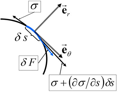
FIGURE 6. Forces at the surface of the liquid. $S=R\delta \theta$, F viscous friction force.

It follows that $\frac{\delta T}{\delta \theta }=\frac{4\mu R^2{\alpha }_i}{{\sigma }_T}\sin \theta$, either: $T=T_0-\frac{4\mu R^2{\alpha }_i}{{\sigma }_T}\cos \theta$, or again:

$T=T_0-\frac{4\mu R{\alpha }_i}{{\sigma }_T}Z[27]$

There is a constant gradient temperature field.

We can therefore give the following result:

A spherical liquid drop of constant density, subjected to a uniform and constant temperature gradient $\overrightarrow{\mathit{G}}=\overline{\mathrm{\nabla }}T$ in an atmosphere at rest, is animated by the internal motion corresponding to the Hill vortex whose velocity of maximum intensity is oriented in the opposite direction to $\overrightarrow{\mathit{G}}$ (Figure 7): $U_{SG}=G{\sigma }_{T}R/2\mu$, G being the thermal gradient $G=dT/dZ$. Then we have:

$U_{\max }=3V_0/2=G{\sigma }_{T}R/2\mu [28]$

FIGURE 7

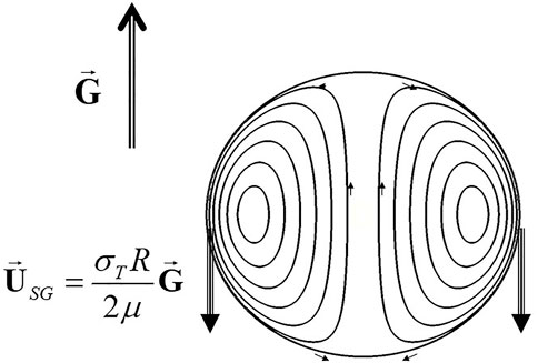
FIGURE 7. Hill vortex generated by a thermal gradient.

3.3 Other Thermo-Capillary Flows

As indicated at the beginning of Section 3.1, Bauer also deals with instabilities in cases other than that of the constant axial thermal gradient.

In his 1985 paper, Bauer (ref.vi) studies the combined effects of Marangoni convection induced by a temperature gradient imposed on the free surface of a liquid sphere and natural convection from the residual microgravity field existing in an orbiting space laboratory. The case of a constant and linearly dependent axial residual gravity field was considered, for which the Stokes equation in the Boussinesq approximation was solved.

A dynamic Bond number derived from the ratio of the Grashof number, and the Reynolds number based on the Marangoni flow is introduced. It makes it possible to determine the predominance of the Marangoni effect if $Bo\to 0$ or of natural convection if $Bo\to \infty$.

The combined effects of Marangoni and natural convection are then studied. Streamlines, radial and angular velocity distributions have been obtained analytically. On the other hand, the isotherms are presented for different temperature distributions imposed on the free surface of the liquid sphere.

The dynamic Bond number introduced is by definition:

$\tilde{B}0=\rho g\beta R^2/\left|{\sigma }_T\right|[29]$

It compares the buoyancy force to the surface tension.

The main gravitational influence is due to the residual acceleration normal to the orbital path, in the plane of the orbit. It is created by the centrifugal acceleration of the space station in circular orbit and the acceleration of Newton.

When g is constant, we write $g=g_0$; for g variable, we have $g={\Omega }_0^{2}R$ where ${\Omega }_0$ is the angular velocity of the center of mass around the center of the earth. Eqs. 12–14 still apply, but Eq. 15 is replaced by

$\overline{\Delta }\left[\overline{\Delta }\psi -\frac{1}{v}\frac{\partial \overline{\psi }}{dt}\right]=-\frac{3{\Omega }_0^2\beta }{v}\left[r^2\frac{\partial T}{\partial r}\sin 0\cos 0+r\frac{\partial T}{\partial \theta }{\cos }^{2}0\right]\sin 0[30]$

where β is the coefficient of thermal expansion of the liquid.

We then use the recurrence formulas of Legendre functions. The calculations lead to expressions of the stream function $\psi \left(r,\theta \right)$ and of the components of the velocity vector $u\left(r,\theta \right),v\left(r,\theta \right)$ according to series expansions of $P_n^0\left(\cos \theta \right)$, and $P_n^1\left(\cos \theta \right)$.

The constants involved in these expressions are to be determined according to the boundary conditions at the surface of the liquid sphere.

In the absence of capillary effects, natural convection is obtained due to the residual gravity present at the location of the space station where the drop is located. We must then distinguish the case where liquid is in a rigid container from the case of the free surface ${\tilde{B}}_0\to \infty$, where we can neglect the thermo-capillary effects.

One also solves the situations where the internal motions of the drop of thermo-capillary origin are important, and we can thus predict the effects of residual gravity on these movements.

With regard to the field of gravity two situations are examined numerically: constant micro-gravity and linearly varying micro-gravity.

As for the field of temperature the field is linear axisymmetric $T-T_0-T_1\cos \theta$, or mixed linear-quadratic $T=T_0+T_1\cos \theta +T_2{\cos }^2\theta$.

Results of the calculations carried out show in Figure 8 the possibility of notable differences with Hill’s vortices. Two-ring configurations of stream surfaces are observed (figures redrawn from the 1985 Bauer article) with a variable residual gravity field and quadratic temperature fields for $T_2/T_1-2$ with ${\tilde{B}}_0-\mathrm{0,10,100}$.

FIGURE 8

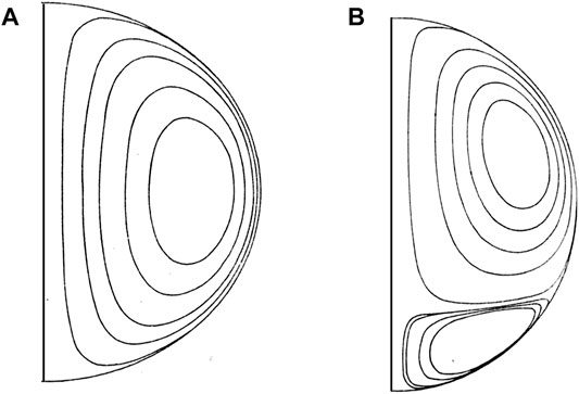
FIGURE 8. Streamlines of vortex rings in the presence of a variable gravity field (redrawn from Bauer 1985): (A) for a linear temperature field and (B) quadratic.

Another figure of the cited article also shows a case with two tore surfaces with a constant residual gravity field, the same quadratic temperature field and ${\tilde{B}}_0==10$.

4 Conclusion

We have presented Hill’s vortex as a structure that can appear inside liquid drops under two circumstances: infinitely uniform external fluid flow, thermal gradient along an axial direction. In both cases the speed of the fluid at the level of the surface of the drop is found to be proportional to the distance from the axis of symmetry.

The physical assumptions were:

1) The sphericity of the drop of constant radius.

2) The liquid: incompressible, expandable, or not, viscous but animated by a rotational motion of inviscid fluid in stationary regime.

3) The external fluid: at rest or animated by a uniform motion far away, inviscid irrotational or locally viscous.

4) Concerning the external liquid fluid interface:

o Simple contact surface or sliding surface,

o Identity of speeds: fluids-surface or only liquid-surface,

o With or without surface tension depending on the temperature. We took care to situate the case of the Hill vortex as a particular case of analysis by series of Legendre functions.

Outlook:

On the Hill vortex, it will be necessary to conclude on the birth and dissipation of this vortex by providing characteristic times (Gharib et al., 1998)^, (Chung, 1982).

On the Marangoni instability in a drop subjected to a radial thermal field with spherical symmetry, we will have to refine our formulation of the problem in spherical coordinates using the articles of Hoefsloot et al. (Hoefsloot et al., 1990)^, (Hoefsloot et al., 1992).

It would be interesting to study the effect of the thermo-capillary vortex on the evaporation of the drop (Shih and Megaridis, 1995)^, (Shih and Megaridis, 1996), in particular in the presence of thermal radiation (Niazmand and Ambarsooz, 2009) or acoustic excitation as we have done with other phenomena (Mauriot and Prud’homme, 2014).

Researchers are already interested in pursuing investigations on the subject⁸.

Data Availability Statement

The original contributions presented in the study are included in the article/Supplementary Materials, further inquiries can be directed to the corresponding author.

Author Contributions

The author confirms being the sole contributor of this work and has approved it for publication.

Conflict of Interest

The authors declare that the research was conducted in the absence of any commercial or financial relationships that could be construed as a potential conflict of interest.

Publisher’s Note

All claims expressed in this article are solely those of the authors and do not necessarily represent those of their affiliated organizations, or those of the publisher, the editors and the reviewers. Any product that may be evaluated in this article, or claim that may be made by its manufacturer, is not guaranteed or endorsed by the publisher.

Supplementary Material

The Supplementary Material for this article can be found online at: https://www.frontiersin.org/articles/10.3389/frspt.2022.835464/full#supplementary-material

Footnotes

¹Paper proposed to Frontiers for “Transport Phenomena in Microgravity”, 13 October 2021.

²Indeed, linking work on microgravity research and space technologies is one of the objectives of the recommendations made during the CNES scientific prospective seminar in July 2004.

³That is to say with no velocity discontinuity at the interface.

⁴Ref. (Germain, 1986), p. 312.

⁵u and v were noted v_r and v_θ in Section 2.1.2.

⁶Unlike Section 2, the spherical drop is not in the presence of a well-defined external flow. This does not have a great importance if one neglects the interaction between the drop and the possible motions in its exterior.

⁷The surface forces are calculated from the speed field of the Hill vortex by introducing a viscosity, whereas this vortex is an inviscid fluid flow. This is not contradictory if we admit that it is a local influence and that the bulk of the flow is changed very little.

⁸In particular at the University of Lomé (Togo), and at the University of Abomey-Calavi (Benin).

References

Abramzon, B., and Sirignano, W. A. (1989). Droplet Vaporization Model for Spray Combustion Calculations. Int. J. Heat. Mass Transf. 32 (N° 9), 1605–1618. doi:10.1016/0017-9310(89)90043-4

CrossRef Full Text | Google Scholar

Bauer, H. F. (1985). Combined Residual Natural and Marangoni Convection in a Liquid Sphere Subjected to a Constant and Variable Micro-gravity Field. Z. Angew. Math. Mech. 65, 461–470. doi:10.1002/zamm.19850651002

CrossRef Full Text | Google Scholar

Bauer, H. F., and Eidel, W. (1987). Marangoni-convection in a Spherical Liquid System. Acta Astronaut. 15, 275–290. doi:10.1016/0094-5765(87)90073-7

CrossRef Full Text | Google Scholar

Bauer, H. F. (1982). Marangoni-convection in a Freely Floating Liquid Sphere Due to Axial Temperature Field. Ing. Arch. 52, 263–273. doi:10.1007/bf00535319

CrossRef Full Text | Google Scholar

Chandrasekhar, S. (1961). Hydrodynamic and Hydromagnetic Stability. Oxford: Clarendon.

Google Scholar

Chung, J. N. (1982). The Motion of Particles inside a Droplet. Trans. ASME 104, 438–445. doi:10.1115/1.3245112

CrossRef Full Text | Google Scholar

Germain, P. (1986). Mécanique. Palaiseau: Ellipses, Ecole Polytechnique.

Google Scholar

Gharib, M., Rambod, E., and Shariff, K. (1998). A Universal Time Scale for Vortex Ring Formation. J. Fluid Mech. 360, 121–140. doi:10.1017/s0022112097008410

CrossRef Full Text | Google Scholar

Hoefsloot, H. C. J., Hoogstraten, H. W., Janssen, L. P. B. M., and Knobbe, J. W. (1992). Growth Factors for Marangoni Instability in a Spherical Liquid Layer under Zero-Gravity Conditions. Appl. Sci. Res. 49, 161–173. doi:10.1007/bf02984176

CrossRef Full Text | Google Scholar

Hoefsloot, H. C. J., Hoogstraten, H. W., and Janssen, L. P. B. M. (1990). Marangoni Instability in a Liquid Layer Confined between Two Concentric Spherical Surfaces under Zero-Gravity Conditions. Appl. Sci. Res. 47, 357–377. doi:10.1007/bf00386244

CrossRef Full Text | Google Scholar

Lamb, H. (1945). Hydrodynamics. Cambridge: Cambridge University Press.

Google Scholar

Mauriot, Y., and Prud’homme, R. (2014). Assessment of Evaporation Equilibrium and Stability Concerning an Acoustically Excited Drop in Combustion Products. Comptes Rendus Mécanique 342, 240–253. doi:10.1016/j.crme.2014.02.004

CrossRef Full Text | Google Scholar

Niazmand, H., and Ambarsooz, M. (2009). Effect of Slip and Marangoni Convection on Single Fuel Droplet Heat-Up in the Presence of Thermal Radiation. Kish Island: ICHEC.

Google Scholar

Prud’homme, R. (2012). Flows and Chemical Reactions. WILEY/ISTE. Available at: http://www.iste.co.uk/index.php?f=a&ACTION=View&id=506.

Google Scholar

Shih, A. T., and Megaridis, C. M. (1995). Suspended Droplet Evaporation Modeling in a Laminar Convective Environment. Combust. Flame 102, 256–270. doi:10.1016/0010-2180(94)00279-2

CrossRef Full Text | Google Scholar

Shih, A. T., and Megaridis, C. M. (1996). Thermocapillary Flow Effects on Convective Droplet Evaporation. Int. J. Heat. Mass Transf. 39 (N°2), 247–257. doi:10.1016/0017-9310(95)00137-x

CrossRef Full Text | Google Scholar

Glossary

D flow rate of a source

$\left({\overrightarrow{e}}_r,{\overrightarrow{e}}_{\theta },{\overrightarrow{e}}_{\varphi }\right)\mathrm{⊸}$ unit basic vectors

K intensity of a doublet

$\overrightarrow{n}$ unit normal

$p,p_{\infty }$ pressure, p at infinite

$P_{l,m}$ legendre polynomial

$r,\theta ,\varphi$ spherical coordinates

R gas constant, radius of a sphere

s curvilinear abscissa

S surface

T absolute temperature

$\overrightarrow{t}$ unit tangent

$U,U_{\infty }$ velocity at surface, velocity at infinity

$\overrightarrow{v},v=\left|\overrightarrow{v}\right|$ velocity vector, velocity modulus

$\left(u,v\right)\mathrm{or}\left(v_r,v_{\theta }\right)$ components of the velocity vector

$\left(x,y,z\right)\left(x_1,x_2,x_3\right)$ cartesian coordinates

$Y_l^m\left(\theta ,\varphi \right)$ spherical harmonic

$\alpha ,{\alpha }_e,{\alpha }_i$ stream function coefficients

$\epsilon$ deformation rate

$\mathit{\Gamma }$ intensity of an irrotational vortex

$\xi =\cos \theta$ intermediate variable

$\rho$ volumic mass

$\sigma$ surface tension

Ω rotation speed

$\overrightarrow{\omega }$ swirl vector

$\psi$ stream fonction

_i, _e flow resp.internal external

t, n resp.tangent, normal to the sphere of radius r

$r,\theta$ resp.radial, tangential